MERGING CLUSTER COLLABORATION: OPTICAL AND SPECTROSCOPIC SURVEY OF A RADIO-SELECTED SAMPLE OF TWENTY NINE MERGING GALAXY CLUSTERS
N. Golovich*1,2, W. A. Dawson2, D. M. Wittman1,3
M. J. Jee1,4, B. Benson1, B. Lemaux1, R. J. van Weeren5, F. Andrade-Santos5, D. Sobral6,7, F. de Gasperin6,8, M. Br¨uggen8, M. Bradaˇc1, K. Finner4, A. Peter9,10,11
Submitted to ApJ Supplement: 3 November 2017 ABSTRACT
Multi-band photometric and multi-object spectroscopic surveys of merging galaxy clusters allow for the characterization of the distributions of constituent dark matter and galaxy populations, constraints on the dynamics of the merging subclusters, and an understanding of galaxy evolution of member galaxies. We present deep photometric observations from Subaru/SuprimeCam and a catalog of ∼5400 spectroscopic cluster members from Keck/DEIMOS across 29 merging galaxy clusters ranging in redshift fromz= 0.07 to 0.55. The ensemble is compiled based on the presence of radio relics, which highlight cluster scale collisionless shocks in the intra-cluster medium. Together with the spectroscopic and photometric information, the velocities, timescales, and geometries of the respective merging events may be tightly constrained. In this preliminary analysis, the velocity distributions of 28 of the 29 clusters are shown to be well fit by single Gaussians. This indicates that radio relic mergers largely occur transverse to the line of sight and/or near apocenter. In this paper, we present our optical and spectroscopic surveys, preliminary results, and a discussion of the value of radio relic mergers for developing accurate dynamical models of each system.
Keywords: Galaxies: clusters: general—dark matter—galaxies: evolution—shock waves
1. INTRODUCTION
Merging galaxy clusters have been established as fruit-ful astrophysical laboratories. In particular, ‘dissociative mergers’ (Dawson et al. 2012), where two galaxy clusters have collided and the effectively collisionless galaxies and dark matter have become dissociated from the collisional ICM which collides and slows during the merger, are a particularly interesting subclass of mergers. They have been used to place tight constraints on the dark mat-ter self-inmat-teraction cross-section (DM; e.g., Clowe et al. 2006;Randall et al. 2008), understand fundamental par-ticle/plasma physics associated with the intra-cluster medium (ICM; e.g., Blandford & Eichler 1987; Marke-vitch et al. 2002; Brunetti & Jones 2014; van Weeren
* nrgolovich@ucdavis.edu
1Department of Physics, University of California, One Shields Avenue, Davis, CA 95616, USA
2Lawrence Livermore National Laboratory, 7000 East Av-enue, Livermore, CA 94550, USA
3Instituto de Astrof´ısica e Ciˆencias do Espa¸co, Universidade de Lisboa, Lisbon, Portugal
4Department of Astronomy, Yonsei University, 50 Yonsei-ro, Seodaemun-gu, Seoul, South Korea
5Harvard-Smithsonian Center for Astrophysics, 60 Garden Street, Cambridge, MA 02138, USA; Clay Fellow
6Leiden Observatory, Leiden University, P.O. Box 9513, 2300 RA Leiden, the Netherlands
7Department of Physics, Lancaster University, Lancaster, LA1 4YB, UK
8Hamburger Sternwarte, Universit¨at Hamburg, Gojen-bergsweg 112, 21029 Hamburg, Germany
9Department of Astronomy, The Ohio State University, 140 W. 18th Avenue, Columbus, OH 43210, USA
10Center for Cosmology and AstroParticle Physics, The Ohio State University, 191 W. Woodruff Avenue, Columbus, OH 43210, USA
11Department of Physics, The Ohio State University, 191 W. Woodruff Avenue, Columbus, Ohio 43210, USA
et al. 2017), and merger related galaxy evolution (e.g., Miller & Owen 2003;Poggianti et al. 2004;Chung et al. 2009; Stroe et al. 2014,2017;Mansheim et al. 2017a,b). These studies have allowed for new and broader under-standing of the content, distribution, and interactions between and within each component. These studies are complicated by: the complexity of the merger properties (mass, dynamics, etc.), the range of disparate observa-tions necessary to form a synoptic understanding of any one merger, and the limited sample size of dissociative mergers to study.
Mergers are complex physical phenomena, where dy-namical parameters such as the merger speed at pericen-ter, the elapsed time since pericenpericen-ter, and the merger geometry are typically unknown. This leaves a vast vol-ume of parameter space that must be considered in any subsequent analysis to properly propagate uncertainty (e.g., Lage & Farrar 2015). The volume of parameter space that must be explored can be shrunk by studying the separate components of the merger as a whole (e.g., Dawson 2013;Ng et al. 2015;Golovich et al. 2016).
Observationally, each component of a merger is probed differently. The DM must be inferred using gravitational lensing techniques that necessitate deep photometric im-ages (seeBartelmann & Schneider 2001;Hoekstra 2013, for a review). The ICM is hot (∼ several keV) and emits thermal bremsstrahlung X-rays (e.g., Cavaliere & Fusco-Femiano 1976) which may be observed spatially and spectroscopically with modern X-ray observatories in orbit. Non-thermal emission from the ICM may be observed with radio telescopes, which reveals complex microphysics of particle acceleration and turbulence (see e.g.,Brunetti et al. 2008). The galaxies may be observed photometrically and spectroscopically. Photometry in multiple bands allow for semi-precise photometric red-shift estimates (see e.g., Ben´ıtez 2000; Bolzonella et al.
2000) and red sequence selection of cluster members (e.g., Kodama & Arimoto 1997). Spectroscopic observations, on the other hand, allow for precise redshift estimation, but these observations are much more expensive and usu-ally result in incomplete surveys of member galaxies. Spectroscopy may also be used to study the effects of the cluster environment on the constituent galaxies via line ratios (e.g.,Baldwin et al. 1981) including AGN and star formation rate studies (e.g.,Moore et al. 1996;Miller & Owen 2003;Stroe et al. 2014;Sobral et al. 2015).
Circa 2012 all dissociative mergers were identified and confirmed using an array of the aforementioned vations. Collecting and analyzing this array of obser-vations was resource intensive, which in large part is the reason for the small sample of dissociative mergers (see Dawson et al. 2012, for a list of the eight known dissociative mergers circa 2012). In recent years, we have implemented new technique of quickly identifying dissociative merging galaxy clusters via detection of en-hanced, diffuse radio emission has become fruitful. Ra-dio relics and raRa-dio halos appear in raRa-dio images between ∼100 MHz and several GHz as Mpc-scale, diffuse radio features. They are thought to trace synchrotron emis-sion from electrons interacting with shocks and turbulent motion (e.g., Brunetti et al. 2008; Feretti et al. 2012), and thus should be associated with dissociative mergers. Magneto-hydrodynamical simulations of cluster mergers confirm this, and can reporduce key features of radio relics (e.g.,Skillman et al. 2013; Vazza et al. 2016). Be-cause radio relic selection of dissociative mergers can be done with a single band wide field survey, while main-taining a high purity (as demonstrated in this paper), it is more economical compared to previous multi-probe selection methods.
Spectroscopic and photometric observations of the galaxies of merging subclusters allow for estimation of the dynamical properties of individual merging systems. We have demonstrated this with a series of studies of in-dividual merger systems (CIZA J2242.8+5301, El Gordo, MACS J1149.5+2223, ZwCl 0008.8+5215, Abell 3411, and ZwCl 2341.1+0000 presented inDawson et al. 2015; Ng et al. 2015; Golovich et al. 2016, 2017; van Weeren et al. 2017; Benson et al. 2017, respectively). The dy-namical models of individual clusters greatly reduce the vast parameter space that simulators must explore to reproduce underlying astrophysics. The presence of ra-dio relics in each of these systems has been shown to greatly improve the precision of dynamical models (Ng et al. 2015;Golovich et al. 2016,2017), and direct study of the underlying shock and radio relics have yielded in-sight into particle acceleration models (e.g., Brunetti & Jones 2014;van Weeren et al. 2017).
In this paper, we outline our photometric and spectro-scopic observations of an ensemble of 29 radio relic merg-ers. In §2 we describe the construction of the ensemble of 29 merging systems. In§3we detail our photometric and spectroscopic observational campaign including the technical details of the observations, data reduction, and data processing. We compile and analyze the redshift global redshift distributions of each system in §4, and we discuss the implications of radio selection and offer conclusions in§5.
We assume a flat ΛCDM universe with H0 = 70 km s−1Mpc−1, ΩM = 0.3, and ΩΛ = 0.7. AB
mag-nitudes are utilized throughout, and all distances are proper.
2. RADIO RELIC SAMPLE
Constraints on the dark matter self-interaction cross-section is one of the driving science cases for this survey. A radio relic selection has a number of potential advan-tages for this science case over other selection methods: (1) it guarantees against the selection of pre-pericentric systems since the presence of a radio relic indicates a shockwave traveling in the ICM due to a major merger; (2) it will disfavor the very youngest post-pericentric sys-tems, which have not had time to generate radio relics, and where the offset between the effectively collisionless galaxies and potentially self-interacting dark matter has not had a chance to increase to a potential maximal offset (Kahlhoefer et al. 2014); (3) it is biased towards selecting mergers in the plane of the sky where any observable off-set between the galaxies, dark matter, and ICM will be maximized (this is also important for other astrophysi-cal studies) (Ensslin et al. 1998); and, (4) as noted in§1, a large sample of dissociative mergers can be prudently compiled.
The first detection of a radio relic in a merging galaxy cluster was in the Coma Cluster (Ballarati et al. 1981). Radio relics were subsequently discovered individually through pointed observations of known merging systems. In the last decade, searches of wide-area radio surveys have increased the rate of detection (e.g., van Weeren et al. 2011a). Several potential radio relics were dis-covered through comparisons of radio surveys with the ROSAT All-Sky Survey catalogs (RASS: Voges et al. 1999). Follow up of these objects resulted in several dis-coveries (van Weeren et al. 2009b,a,2010,2011b,2012b,a, 2013). Our sample begins with these radio relics, along with additional radio relics known by September 2011 listed in Table 3 of Feretti et al. (2012). Each of these clusters contain low surface brightness, steep-spectrum, polarized, and extended radio sources that lie at the pe-riphery of the cluster (for individual observational papers see references therein). Relics classified as having a round morphology were discarded since they are likely radio phoenixes rather than Mpc scale cluster shocks. Radio phoenixes are generally associated with aged radio galaxy lobes that are re-energized through compression or other mechanisms (e.g.,de Gasperin et al. 2015b). We imposed cuts designed to enable spectroscopic and weak lensing followup. Systems at very low redshift are not efficient lenses, so we eliminate clusters at z < 0.07. We also eliminate systems not observable from the Mauna Kea observatories (δ < −31◦) from which we were awarded
observational time. To this list, we added three ad-ditional radio relic systems that have appeared in the literature and pass the same selection criteria (MACS J1149.5+2223, PSZ1 G108.18-11.5 and ZwCl 1856+6616, hereafter MACSJ1149, PSZ1G108 and ZwCl1856, re-spectively:Bonafede et al. 2012;de Gasperin et al. 2014, 2015a). Finally, we added one of the radio phoenix relics (Abell 2443, hereafter A2443) to our spectroscopic sur-vey due to a gap in an observing run. In total, our sample contains 29 systems listed in Table 1.
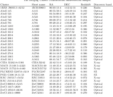
Table 1
The Merging Cluster Collaboration radio-selected sample.
Cluster Short name RA DEC Redshift Discovery band 1RXS J0603.3+4212 1RXSJ0603 06:03:13.4 +42:12:31 0.226 Radio
Abell 115 A115 00:55:59.5 +26:19:14 0.193 Optical Abell 521 A521 04:54:08.6 -10:14:39 0.247 Optical Abell 523 A523 04:59:01.0 +08:46:30 0.104 Optical Abell 746 A746 09:09:37.0 +51:32:48 0.214 Optical Abell 781 A781 09:20:23.2 +30:26:15 0.297 Optical Abell 1240 A1240 11:23:31.9 +43:06:29 0.195 Optical Abell 1300 A1300 11:32:00.7 -19:53:34 0.306 Optical Abell 1612 A1612 12:47:43.2 -02:47:32 0.182 Optical Abell 2034 A2034 15:10:10.8 +33:30:22 0.114 Optical Abell 2061 A2061 15:21:20.6 +30:40:15 0.078 Optical Abell 2163 A2163 16:15:34.1 -06:07:26 0.201 Optical Abell 2255 A2255 17:12:50.0 +64:03:11 0.080 Optical Abell 2345 A2345 21:27:09.8 -12:09:59 0.179 Optical Abell 2443 A2443 22:26:02.6 +17:22:41 0.110 Optical Abell 2744 A2744 00:14:18.9 -30:23:22 0.306 Optical Abell 3365 A3365 05:48:12.0 -21:56:06 0.093 Optical Abell 3411 A3411 08:41:54.7 -17:29:05 0.163 Optical CIZA J2242.8+5301 CIZAJ2242 22:42:51.0 +53:01:24 0.189 X-ray MACS J1149.5+2223 MACSJ1149 11:49:35.8 +22:23:55 0.544 X-ray MACS J1752.0+4440 MACSJ1752 17:52:01.6 +44:40:46 0.365 X-ray PLCKESZ G287.0+32.9 PLCKG287 11:50:49.2 -28:04:37 0.383 SZ PSZ1 G108.18-11.53 PSZ1G108 23:22:29.7 +48:46:30 0.335 SZ RXC J1053.7+5452 RXCJ1053 10:53:44.4 +54:52:21 0.072 X-ray RXC J1314.4-2515 RXCJ1314 13:14:23.7 -25:15:21 0.247 X-ray ZwCl 0008.8+5215 ZwCl0008 00:08:25.6 +52:31:41 0.104 Optical ZwCl 1447+2619 ZwCl1447 14:49:28.2 +26:07:57 0.376 Optical ZwCl 1856.8+6616 ZwCl1856 18:56:41.3 +66:21:56.0 0.304 Optical ZwCl 2341+0000 ZwCl2341 23:43:39.7 +00:16:39 0.270 Optical
et al. 1998). This is a reasonable redshift range for lens-ing follow-up, and also has the advantage of mapplens-ing given physical separations to substantial angular separa-tions for spatial analysis of cluster components.
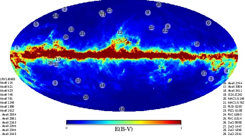
The radio selection strategy brings challenges in terms of obtaining spectroscopy and lensing followup. Because radio surveys have gone right through the galactic plane, many of the systems suffer more extinction than is typ-ical in visible-wavelength surveys. The all sky galactic dust extinction map is presented in Figure1 with all 29 systems in our sample. The most extreme example is CIZAJ2242 with AV ≈1.4 (the approximation sign
em-phasizes that the extinction varies over the field;Schlegel et al. 1998). Dawson et al.(2015) describes the success of the position-dependent extinction corrections applied to that system in terms of yielding uniform color selection of cluster members, and Jee et al. (2015) demonstrates that weak lensing can be efficiently measured despite the extinction. The low galactic latitude also affected the spectroscopy not only through extinction but also by causing more slits to be wasted on stars. A contribut-ing factor in some cases was the poor quality of imagcontribut-ing available at the time of slit mask design. Blended binary stars were not rejected in morphological cuts, and con-stituted a substantial contamination. The next most ex-tincted systems in the sample are A2163 and ZwCl0008, for whichAV ∼0.8. We therefore expect the lensing and
galaxy analyses of most of the systems in this sample to exceed the quality of those for CIZAJ2242. We have corrected our photometry for extinction throughout.
The resulting 29 systems are listed in Table1. For each system, the following milestones are to be achieved for
each cluster:
• Observations including spectroscopic, ground based wide field photometric, space based pointed photometric, X-ray and radio
• Optical analysis to estimate the number and loca-tion of subclusters
• Redshift analysis to estimate line of sight velocity information of subclusters
• X-ray and radio analysis of shocks and radio relics including polarization measurements
• Weak lensing analysis to find location and mass of subclusters
• Dynamical analysis
Galactic
1 2 3 4 5 6 7 8 9 1011 12 13 14 15 16 17 18 19 20 21 22 23 24 25 26 27 28 29 Mollweide view0
E(B-V)
11. 1RXS J0603 2. Abell 115 3. Abell 521 4. Abell 523 5. Abell 746 6. Abell 781 7. Abell 1240 8. Abell 1300 9. Abell 1612 10. Abell 2034 11. Abell 2061 12. Abell 2163 13. Abell 2255 14. Abell 2345 15. Abell 2443
[image:4.612.62.551.73.348.2]16. Abell 2744 17. Abell 3365 18. Abell 3411 19. CIZA J2242 20. MACS J1149 21. MACS J1752 22. PLCK G287 23. PSZ1 G108 24. RXC J1053 25. RXC J1314 26. ZwCl 0008 27. ZwCl 1447 28. ZwCl 1856 29. ZwCl 2341
Figure 1. Galactic dust extinction map (Schlegel et al. 1998) with overlaid positions of the 29 systems in our sample.
3. OPTICAL IMAGING AND SPECTROSCOPIC OBSERVATIONAL CAMPAIGN
3.1. Survey Goals and Requirements
The goal of the optical imaging survey is to obtain lensing quality, wide-field imaging in at least two photo-metric bands. The two filters are chosen to straddle the 4000˚A break in order to select cluster members photo-metrically via red sequence relations. Furthermore, our weak lensing method makes use of these red sequence relations in order to select background galaxies for lens-ing studies (Jee et al. 2015,2016; Golovich et al. 2017). Additionally, for clusters that our SuprimeCam observa-tions came before our DEIMOS observaobserva-tions, we made use of the SuprimeCam images for spectroscopic target selection (see§3.3.1). Many clusters have archival imag-ing that we have obtained. We observed 18 systems with Subaru/SuprimeCam to complete the photometric sur-vey.
The spectroscopic survey has a goal of obtaining∼200 member galaxy velocities in each system. We used red-shifts from the literature when available in order to re-duce the amount of new observations required. When obtaining new spectra, we designed observations to also meet the goal of enabling studies of recent star forma-tion and ultimately the link between mergers and star formation. We achieve this by adjusting the observed wavelength range for each cluster to the emitted wave-length range from Hβ to Hα for clusters with z . 0.3 and [OII] to [OIII] for clusters with z&0.3. The data available for star formation studies therefore varies from cluster to cluster depending on the number of previously published redshifts and the redshift of the cluster. Ad-ditional observations were required for 18 systems with
many having no more than a handful of previously pub-lished member redshifts. In the following subsections we will detail the targeting, observing, and data reductions of our optical and spectroscopic surveys.
3.2. Subaru/SuprimeCam Observations
We observed 18 clusters over four nights using the 80 Megapixel SuprimeCam (Miyazaki et al. 2002) camera on the Subaru Telescope on Mauna Kea. Table 2 summa-rizes these observations. The basic strategy is to achieve weak lensing quality in one filter and obtain a second fil-ter to define the color of detected objects by straddling the 4000 ˚A break. For the lensing quality image, the ex-posure time was 2880 s (8×360 s) and we rotated the field between each exposure by 15◦ in order to distribute the bleeding trails and diffraction spikes from bright stars az-imuthally to be later removed by median-stacking. This scheme enabled us to maximize the number of detected galaxies, especially for background source galaxies for weak lensing near stellar halos or diffraction spikes. In the second and third filters (g and/or i), the exposure time was 720 s (4×180 s). These exposures were rotated by 30◦ from exposure to exposure for the same reason as above. In order to efficiently fill the time of each ob-serving night, we added a third band to several clusters. The actual observing times may vary due to real-time changes to the observational plan due to unexpected lost time.
Table 2
Merging Cluster Collaboration radio-relic selected Subaru/SuprimeCam survey.
Cluster Filter Date Seeing (arcsec) Exposure (s)
1RXS J060313.4+421231 g 2014 February 25 0.57 720 1RXS J060313.4+421231 r 2014 February 25 0.57 2880 1RXS J060313.4+421231 i 2014 February 25 0.50 720
Abell 523 g 2014 February 26 1.00 720
Abell 523 r 2014 February 26 0.78 2880
Abell 746 g 2014 February 26 0.88 720
Abell 746 r 2014 February 26 1.01 2880
Abell 1240 g 2014 February 25 0.67 720
Abell 1240 r 2014 February 25 0.58 2880
Abell 1300 g 2014 February 26 0.89 720
Abell 1300 r 2014 February 26 0.88 2160
Abell 2061 g 2013 July 13 0.68 720
Abell 2061 r 2013 July 13 0.67 2520
Abell 2061 i 2013 July 13 0.60 2676
Abell 2061 i 2014 February 26 0.65 720
Abell 3365 g 2014 February 25 0.97 720
Abell 3365 r 2014 February 25 0.71 2880
Abell 3365 i 2014 February 25 0.62 720
Abell 3411 g 2014 February 25 0.80 720
Abell 3411 r 2014 February 25 0.82 2880
Abell 3411 i 2014 February 25 0.77 720
CIZA J2242.8+5301 g 2013 July 13 0.63 720
CIZA J2242.8+5301 i 2013 July 13 0.55 3400
MACS J175201.5+444046 g 2013 July 13 0.62 720
MACS J175201.5+444046 r 2013 July 13 0.64 1440
MACS J175201.5+444046 i 2013 July 13 0.63 2520
MACS J175201.5+444046 i 2014 February 26 0.73 1260 PLCKESZ G287.0+32.9 g 2014 February 26 0.81 720 PLCKESZ G287.0+32.9 r 2014 February 26 0.97 2880 PSZ1 G108.18-11.53 g 2015 September 12 0.65 1440 PSZ1 G108.18-11.53 r 2015 September 12 0.55 2520
RXC J1053.7+5452 g 2014 February 26 0.83 720
RXC J1053.7+5452 r 2014 February 26 0.92 720
RXC J1314.4-2515 g 2014 February 25 0.86 720
RXC J1314.4-2515 r 2014 February 25 0.71 2880
RXC J1314.4-2515 NB814 2014 February 25 0.77 1000
ZwCl 0008.8+5215 g 2013 July 13 0.52 720
ZwCl 0008.8+5215 r 2013 July 13 0.57 2880
ZwCl 1447+2619 g 2014 February 26 0.91 720
ZwCl 1447+2619 r 2014 February 26 0.76 2880
ZwCl 1447+2619 i 2014 February 26 0.55 720
ZwCl 1856+6616 g 2015 September 12 0.70 720
ZwCl 1856+6616 r 2015 September 12 0.65 2520
ZwCl 2341+0000 g 2013 July 13 0.49 720
set of archival images for these clusters since we only re-quired two bands of imaging in order to define the color and complete a color–magnitude selection. We utilized the deepest images available that satisfy this requirement ensuring good seeing conditions.
3.2.1. Subaru/SuprimeCam: Data Reduction
The CCD processing (overscan subtraction, flat-fielding, bias correction, initial geometric distortion rec-tification, etc) were carried out with the SDFRED2 pack-age (Ouchi et al. 2004). Much of the archival data re-quired the first version of this pipeline (SDFRED1:Yagi et al. 2002). We refine the geometric distortion and World Coordinate System (WCS) information using the SCAMP software (Bertin 2006). The Two Micron All Sky Survey (Skrutskie et al. 2006, 2MASS; ) catalog was selected as a reference when the SCAMP software was run except for clusters covered by the Sloan Digital Sky Survey (SDSSAdelman-McCarthy et al. 2007), for which the Data Release 5 catalogs were used. We also rely on SCAMP to calibrate out the sensitivity variations across different frames. For image stacking, we ran the SWARP software (Bertin et al. 2002) using the SCAMP result as input. We first created median mosaic images and then used it to mask out pixels (3σ outliers) in individual frames. These masked frames were weight-averaged to generate the final mosaic, which is used for the scientific analyses hereafter. Two example images are presented in Figure2.
3.2.2. Subaru/SuprimeCam: Photometric Catalog Generation
Object detection is achieved with Source Extractor (Bertin & Arnouts 1996) in dual image mode using the deepest image for detection. The blending threshold pa-rameterBLEND-NTHRESHis set to 32 with a minimal con-tact DEBLEND MINCONT of 10−4. We employ reddening values from Schlafly & Finkbeiner (2011) to correct for dust extinction, which are listed in Tables2 and3. Zero points were transferred from SDSS for the overlapping clusters and transferred to the clusters outside the SDSS footprint observed on the same night with SuprimeCam accounting for atmospheric extinction related to the air-mass differences of our observations. Atmospheric ex-tinction values for Mauna Kea were taken from Buton et al.(2013).
Since the sample has relatively low redshift, it is ex-pected for cluster members to have high S/N and corre-spondingly good photometry. We enforce that potential cluster member objects have uncertainties in their mag-nitudes of less than 0.5 magmag-nitudes, and we remove all objects brighter than the BCG, which we have identified spectroscopically in each cluster. These cuts eliminate most bright foreground galaxies and stars as well as false detections at extremely faint magnitudes. Only objects within R200 (as determined from our redshift analysis and scaling relationsEvrard et al. 2008;Duffy et al. 2008) of the center of the cluster are retained. This limits the vignetting of the edges as well as removes spurious de-tections near the edge of the field.
3.3. Keck/DEIMOS Observations
We conducted a spectroscopic survey utilizing the DEIMOS multi-object spectrograph (Faber et al. 2003)
on the Keck II telescope at the W. M. Keck Observa-tory on Mauna Kea over the following nights: 26 Jan-uary 2013, 14 July 2014, 5 September 2014, 3-5 Decem-ber 2013 (half nights), 22-23 June 2014, 15 February 2015, and 13 December 2015. In total, 54 slit masks were observed. Each was milled with 100 wide slits and
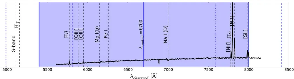
utilized the 1200 line mm−1 grating, which results in a pixel scale of 0.33 ˚A pixel−1 and a resolution of ∼ 1 ˚A (50 km s−1). For clusters with a redshift below 0.3, the grating was tilted to observe the following spectral fea-tures: Hβ, [O III], Mg I (b), Fe I, Na I (D), [O I], Hα, and the [NII] doublet. A typical wavelength coverage of 5400 ˚A to 8000 ˚A is shown in Figure 3 for a galaxy ob-served in CIZAJ2242. The actual wavelength coverage may be shifted by ∼ ±400˚A depending where the slit is located along the width of the slit mask. This spectral setup enables us to also study the star formation prop-erties of the cluster galaxies; see related work bySobral et al.(2015). For higher redshift clusters (above 0.3), the grating was tilted to instead cover the following spectra features: [OII], Ca(H), Ca(K), Hδ, G-band, Hγ, Hβ, and [OIII]. The position angle (PA) of each slit was chosen to lie between±5◦to 30◦of the slit mask PA to achieve
op-timal sky subtraction during reduction with the DEEP2 version of the spec2d package (Newman et al. 2013). In general, for each mask we took three∼900 s exposures ex-cept for a few cases where a few extra minutes at the end of the night were spent on an individual mask or when weather altered our observation plans in the middle of the night. In total, 54 slit masks were observed with a total of ∼7000 slits over the course of the spectroscopic survey.
3.3.1. Keck/DEIMOS: Target Selection
Our primary objective for the spectroscopic survey was to maximize the number of cluster member spectroscopic redshifts in order to detect merging substructure within
R200. For each slit mask, the best imaging data available were utilized. For one third of the clusters this was our own SuprimeCam imaging from our simultaneous wide field imaging survey (see §3.2). In the cases where this was unavailable at the time of our spectroscopic survey planning, we used the next best imaging at our disposal. SDSS Data Release 5 catalogs were utilized (Adelman-McCarthy et al. 2007) for ten of the clusters, and for six of the clusters, this was INT WFC data presented in (van Weeren et al. 2011c). For the remaining two clus-ters, Digitized Sky Survey (DSS: Djorgovski et al. 1992) imaging was utilized. For all imaging except the SDSS data, for which a photometric redshift selection was em-ployed, a red sequence technique was utilized to select likely cluster members to create a galaxy number density map. The slit masks were then oriented to maximize the number of cluster members in the high red sequence den-sity regions. Priors from the literature were also utilized in the placement of slit masks (e.g. lensing maps, X-ray surface brightness, radio relics, etc).
imag-Table 3
Archival imaging from Subaru/SuprimeCam utilized in this study.
Cluster Filter Date Exposure (s)
Abell 115 V 2003 September 25, 2005 October 03 1530
Abell 115 i 2005 October 03 2100
Abell 521 V 2001 October 14 1800
Abell 521 R 2001 October 15 1620
Abell 781 V 2010 March 14, 15 3360
Abell 781 i 2010 March 15 2160
Abell 2034 g 2005 April 11 720
Abell 2034 R 2005 April 11, 2007 June 19 12880
Abell 2163 V 2009 April 30 2100
Abell 2163 R 2008 April 07 4500
Abell 2255 B 2007 August 14 1260
Abell 2255 R 2007 August 14 2520
Abell 2345 V 2010 June 10, 2010 November 10 3600
Abell 2345 i 2005 October 03 2100
Abell 2744 B 2013 July 16 2100
Abell 2744 R 2013 July 15 3120
MACS J1149 V 2003 April 05 2520
[image:7.612.51.561.294.556.2]MACS J1149 R 2003 April 05, 2005 March 05, 2010 March 18 5490
Figure 2. Example Subaru/SuprimeCam images of the central regions of A2061 (left) and A2744 (right). A2061 is displayed using our g, r, and i band images while A2744 is displayed using archival B, R, and Z images. Note that the i-band image for A2061 and the Z-band image for A2744 were used only to make these true-color images. These images were combined using the trilogy software (Coe et al. 2012).
ing; thus, several of our slit masks were highly contam-inated with stars. For example, for CIZAJ2242, which sits near the plane of the galaxy, has a stellar density nearly three times that of cluster members. When se-lecting targets, we divided our potential targets into a bright red sequence sample (Sample 1; r <22.5) and a faint red sequence sample (Sample 2; 22.5< r <23.5). We first filled our mask with as many Sample 1 targets as possible, then filled in the remainder of the mask with Sample 2 targets. While we preferentially targeted likely red sequence cluster members it was not always possi-ble to fill the entire mask with these galaxies, in which
case we would place a slit on bright blue cloud galaxies in the field. For the SDSS targeted galaxies, we selected from galaxies satisfyingzphotwithin±0.05(1 +zcluster) of the cluster redshift and prioritized bright galaxies with a luminosity weighted selection. In these cases, Sample 2 was composed of any other bright objects outside the photometric selection.
We used the DSIMULATOR package12 to design each
Table 4
Merging Cluster Collaboration radio-relic selected spectroscopic survey.
Slitmask Date Target Imaging Exposure (s) Wavelength (˚A) Slits
1RXSJ0603-1 2013 January 16 WFC 3000 6200 105
1RXSJ0603-2 2013 January 16 WFC 3000 6200 100
1RXSJ0603-3 2013 September 5 WFC 3600 7000 98
1RXSJ0603-4 2013 September 5 WFC 3600 7000 87
A115-1 2014 June 22 SDSS 2500 6900 176
A115-2 2014 June 23 SDSS 2400 6900 142
A523-1 2013 January 16 WFC 3000 6200 99
A523-2 2013 December 4 WFC 2700 6200 94
A523-3 2015 February 16 WFC 2700 6300 111
A746-1 2013 January 16 SDSS 3600 6200 110
A1240-1 2013 December 3 SDSS 2700 6850 120
A1240-2 2015 February 16 SDSS 2700 6820 164
A1612-1 2015 February 16 SDSS 1200 6750 186
A2034-1 2013 July 14 SDSS 2700 6700 158
A2443-1 2014 June 22 SDSS 2400 6400 153
A2443-2 2014 June 23 SDSS 2400 6400 163
A3365-1 2013 January 16 WFC 2700 6200 68
A3365-2 2013 January 16 WFC 2400 6200 66
A3365-3 2013 December 3 WFC 2700 6300 63
A3365-4 2015 February 16 SC 2700 6200 160
A3411-1 2013 December 3 WFC 2700 6650 132
A3411-2 2013 December 3 WFC 2700 6650 127
A3411-3 2013 December 4 WFC 2700 6650 128
A3411-4 2013 December 4 WFC 2700 6650 131
A3411-5 2015 December 13 SC 3600 6650 142
CIZAJ2242-1 2013 July 14 WFC 2700 6700 148
CIZAJ2242-2 2013 July 14 WFC 2700 6700 126
CIZAJ2242-3 2013 September 5 SC 2700 7000 90
CIZAJ2242-4 2013 September 5 SC 2700 7000 106
MACSJ1752-1 2013 July 14 SDSS 2700 6700 155
MACSJ1752-2 2013 July 14 SDSS 2700 6700 119
MACSJ1752-3 2013 September 5 SDSS 3600 7000 114
MACSJ1752-4 2013 September 5 SDSS 2700 7000 118
PLCKG287-1 2015 February 16 SC 3900 7950 207
PLCKG287-2 2015 February 16 SC 2700 7950 185
PLCKG287-3 2015 February 16 SC 2700 7950 193
PSZ1G108-1 2014 June 22 DSS 1800 7400 198
PSZ1G108-2 2014 June 23 DSS 1800 7650 168
RXCJ1053-1 2013 January 16 SDSS 2803 6200 113
RXCJ1053-2 2013 December 3 SDSS 2700 6200 84
RXCJ1053-3 2013 December 4 SDSS 2430 6200 98
RXCJ1314-1 2015 February 16 SC 2520 7120 196
RXCJ1314-2 2015 February 16 SC 2520 7120 207
ZwCl0008-1 2013 January 16 WFC 2063 6200 81
ZwCl0008-2 2013 July 14 WFC 2700 6700 81
ZwCl0008-3 2013 September 5 WFC 2700 7000 75
ZwCl0008-4 2013 September 5 WFC 3600 7000 73
ZwCl1447-1 2014 June 22 SDSS 1520 7850 149
ZwCl1447-2 2014 June 23 SDSS 1053 7850 138
ZwCl1856-1 2014 June 22 DSS 1800 7400 150
ZwCl1856-2 2014 June 23 DSS 1800 7400 101
ZwCl2341-1 2013 July 14 SDSS 2700 6700 130
ZwCl2341-2 2013 July 14 SDSS 2700 6700 131
ZwCl2341-3 2013 September 5 SDSS 2700 7000 148
Note. — Target Imaging codes: WFC=Issac Newton Telescope Wide Field Camera presnted invan Weeren et al.(2011c), SDSS=Sloan Digital Sky Survey (e.g.,Alam et al. 2015), DSS=Palomar Observatory Digitized Sky Survey (Djorgovski et al. 1992), SC=Subaru/SuprimeCam imaging (see§3.2)
as possible then filling in the remaining area of the slit mask with target candidates from Sample 2. We manu-ally edited the automated target selection to increase the number of selected targets, e.g. by selecting another tar-get between tartar-gets selected automatically by DSIMU-LATOR if the loss of sky coverage was acceptably small.
3.3.2. Keck/DEIMOS: Data Reduction
Figure 3. ReprintedFigure 2 ofDawson et al.(2015). Example spectral coverage of the Keck/DEIMOS observations (shaded blue region) for a low redshift (z≤0.3) cluster, along with the redshifted location of common cluster emission and absorption features (black dashed lines). The blue dot-dash pair and the blue dashed pair of lines show the variable range depending on where the slit was located along the width of the slit mask. The solid black line shows an example galaxy spectrum from our DEIMOS survey.
the target, containing the summed flux at each wave-length in an optimized window. The spec1d pipeline then fits template spectral energy distributions (SED’s) to each one-dimensional spectrum and estimates a cor-responding redshift. There are SED templates for var-ious types of stars, galaxies, and active galactic nuclei. We then visually inspect the fits using the zspec soft-ware package (Newman et al. 2013), assign quality rank-ings to each fit (following a convention closely related to Newman et al. 2013), and manually fit for redshifts where the automated pipeline failed to identify the cor-rect fit. The highest quality galaxy spectra (Q=4) have a mean signal-to-noise-ratio (SNR) of 10.7 per pixel, while the minimum quality galaxy spectra used on our redshift analysis (Q=3) have a mean SNR of 4.9 per pixel. Note that the SNR estimates are dominated by the continuum of a spectroscopic trace and an emission line galaxy may be of high quality but very low mean SNR (for example the mean SNR of a Q=4 emission line galaxy is 1.2 de-spite detection of Hα and Hβ or [OIII] in most cases). An example of one of the reduced spectra is reprinted from Figure 2 of Dawson et al. (2015) in Figure 3 and more are shown in a related galaxy evolution paper So-bral et al.(2015).
In Table A.1, we present ∼5800 high quality galax-ies and stars from our spectroscopic survey along with matched photometry from our photometric survey.
3.3.3. Archival Spectroscopy
To augment our spectroscopic survey, we completed a detailed literature review of published spectroscopic red-shifts of cluster members for the 29 systems in the en-semble. We compiled spectroscopic galaxies in each field using using the NASA/IPAC Extragalactic Database13
(NED). For each system we considered galaxies within 5 Mpc of the cluster center and within ±10,000 km s−1 of the mean cluster redshift to be sufficiently plausible members. Many galaxies published in the literature also appear in NED, so we cross matched and eliminated duplicate galaxies and prioritized originally published galaxies over NED matches.
We combine all known redshifts (from NED, the liter-ature, and our DEIMOS survey) in the cluster fields and
check for duplicates using the Topcat (Taylor 2005) soft-ware using the sky function with a 100 tolerance. These
combined catalogs of unique spectroscopically confirmed objects are studied in §4. In Table 5, the numbers of spectroscopic redshifts from the literature review and DEIMOS survey are reported.
4. REDSHIFT ANALYSIS
In this section we describe the process of selecting spec-troscopic cluster members from our combined redshift catalogs (see Table 4and5).
4.1. Spectroscopic Catalog Generation
We cut each spectroscopic catalog to only include ob-jects withinR200in projected space and to within ¯v±3σv,
where ¯vis the average line of sight velocity andσv is the
cluster velocity dispersion. This is accomplished with an iterative process starting with 5 Mpc and 10,000 km s−1 and shrinking the radius and velocity window until an equilibrium catalog is achieved. This reduces the chance of inclusion of galaxies that are uninvolved in the merger. An instructive example is Abell 2061, where Abell 2067 is∼2.7 Mpc (300) to the northeast and at a similar red-shift, but uninvolved in the merger. The iterative shrink-ing aperture was able to eliminate galaxies from A2067 from the redshift catalog despite being at a similar red-shift because it is outside of R200. A second example is Abell 523 (z∼0.1), which has two background groups at
z∼0.14 withinR200 in projection (Girardi et al. 2016).
4.2. One Dimensional Redshift Analysis
We display the one dimensional redshift distribution for 1RXSJ0603 in Figure 4. An analogous figure for the remaining 28 systems is presented the appendix. The corresponding normalized Gaussian distribution is overlaid with the cluster redshift and velocity dispersion given by the biweight and bias corrected 68% confidence intervals. We implement the biweight statistic based on 10,000 bootstrap samples of the member galaxies and calculate the bias-corrected 68% confidence limits for the redshift and velocity dispersion from the bootstrap sam-ple. This method is more robust to outliers than the dispersion of the Gaussians generated by our statistical model (Beers et al. 1990).
Table 5
Breakdown of spectroscopy from our DEIMOS and the literature
Cluster Unique DEIMOS Unique Literature References
1RXSJ0603 387 0 —
A115 255 76 B83, Z90, B07, 2MASS, SDSS
A521 0 193 M00, F03
A523 268 61 G16
A746 94 6 2MASS, SDSS
A781 0 875 G05, SDSS
A1240 197 151 B09, 2MASS, SDSS
A1300 0 270 P97, Z12
A1612 83 39 SDSS
A2034 130 129 SDSS, O14
A2061 0 404 SDSS
A2163 0 407 M08
A2255 0 406 SDSS
A2345 0 103 B10
A2443 253 17 SDSS
A2744 0 695 C87, B06, O11
A3365 313 33 K98, 6dF
A3411 550 0 vW17
CIZAJ2242 447 0 D15
MACSJ1149 0 591 SDSS, E14
MACSJ1752 432 0 —
PLCKG287 666* 0 —
PSZ1G108 290 0 —
RXCJ1053 232 144 SDSS
RXCJ1314 286 18 V02
ZwCl0008 278 0 G17
ZwCl1447 212 0 —
ZwCl1856 214 0 —
ZwCl2341 324 62 SDSS, B13
Note. — Reference codes in Column 4: B83=Beers et al. (1983), Z90=Zabludoff et al.(1990), B07=Barrena et al. (2007), 2MASS=Skrutskie et al. (2006), SDSS=Alam et al. (2015), M00=Maurogordato et al. (2000), F03=Ferrari et al. (2003), G16=Girardi et al.(2016), G05=Geller et al. (2005), B09=Barrena et al.(2009), P97=Pierre et al.(1997), Z12=Ziparo et al.
(2012), O14=Owers et al.(2014), M08=Maurogordato et al.(2008), B10=Boschin et al.(2010), C87=Couch & Sharples(1987), B06=Boschin et al.(2006), O11=Owers et al.(2011), K98=Katgert et al.(1998), 6dF=Jones et al.(2005), vW17=van Weeren et al.(2017), D15=Dawson et al.(2015), E14=Ebeling et al.(2014), V02=Valtchanov et al.(2002), G17=Golovich et al.(2017), B13=Boschin et al. (2013)
Note. — * 317 unique redshifts were obtained from VLT VIMOS Obs ID. 094.A-0529, PI M. Nonino
The results of this analysis is displayed in Figure 4 and in the Appendix for the other systems. We generally find good agreement between the spectroscopic data and sin-gle Gaussian distributions, which implies that the merg-ing subclusters have line of sight velocity differences that are small compared to the velocity dispersion. The low-est p-value for the KS tlow-est is 0.007 for Abell 781, which is known to be composed of several subclusters with large velocity differences (Geller et al. 2005).
We also fit increasing numbers of Gaussians to the one-dimensional redshift distributions of each cluster utilizing an expectation-maximization Gaussian mixture model (EM-GMM) method from the Sci-Kit Learn python mod-ule. We varied the number of Gaussians from one to seven for each cluster. A one Gaussian model was strongly preferred for 27 of the 29 clusters according to the Bayesian Information Criterion (BIC). For A3365, the one Gaussian model was only slightly favored over a two Gaussian model, and for A781, a two halo model was preferred strongly.
In a second paper (Golovich et al., in preperation), we will study the three-dimensional distribution of galaxies.
5. DISCUSSION
5.1. Analysis of the Spectroscopic Survey
1RXSJ0603
KS-test: p=0.61
z=0.22631±0.00038
v
=1488±60 kms
1 [image:11.612.59.287.69.239.2]N=242
Figure 4. Redshift distribution for 1RXSJ0603 based on our DEIMOS spectroscopic survey. Galaxies are selected with a shrink-ing 3D aperture until a stable set of galaxies within R200and±3σv
is achieved. The global redshift analysis using the biweight statis-tic and bias corrected 68% confidence limits are presented in the panel. The p-value for a KS-test for Gaussianity is presented as well. The panel width is 12,000 km s−1centered on the cluster red-shift. Bins are 300 km s−1 at the cluster redshift. The analogous distributions for the other 28 systems in our sample are located in the appendix.
The biggest indication of the effect of the target imag-ing quality on the spectroscopic survey is with the frac-tion of targeted objects that yielded a secure redshift of a cluster member, which was our primary goal. In Table 6, the ∼7000 targeted objects are broken down by the type of object detected. Across the survey, 77% of all targeted objects yielded a secure redshift estimate. Of these, 49% were cluster galaxies. The largest sources of contaminants were background galaxies (26%) and stars (18%).
Background galaxies detected at higher frequency with photometric redshift targeting. Detection of these ob-jects also decreased with the redshift of the cluster. A substantial fraction of stars were detected in a few fields that had either sub-par imaging for target selection, or have low galactic latitude. The effect of imaging quality with regards to stellar contamination is evident in the five A3411 slit masks. The first four were observed us-ing WFC targetus-ing, and the fraction of stars increased for successive slit masks as the best member candidates were depleted by earlier masks. For the fifth slit mask, Subaru/SuprimeCam was utilized for targeting, and the fraction of stars decreased substantially. The trade off was a larger fraction of background galaxies, which is explained by the increased depth of the imaging. One benefit of the background galaxy redshift determination is for developing training sets for weak lensing source selection. Furthermore, gravitational lensing is compli-cated by massive structures along the line of sight, and over densities of background galaxies may help discover these types of massive background structures; however, the spectroscopic survey was not designed to detect such systems, so any detection will be serendipitous. Fore-ground galaxies accounted for only 6% of secure red-shifts, and these were predominately detected in higher redshift cluster fields. Finally, 305 objects were detected serendipitously; i.e., a single slit had one or more traces
in addition to the targeted object. These were predom-inately detected in low galactic latitude fields and were composed of stars; although, ∼50 cluster galaxies were detected in this manner across the survey.
5.2. Cluster Redshift Histograms
The presence of radio relics in merging galaxy clusters constitutes a strong prior for ongoing merging activity. Given this, these 29 merging clusters are expected to be composed of two or more subclusters. However, 28 of the 29 systems are well fit by a single Gaussian (p >0.05). There are two potential explanations for this, which are not mutually exclusive: 1) radio relics indicate a merger occurring within the plane of the sky (transverse to the line of sight), and/or 2) radio relics indicate a merger observed near apocenter.
Based on the redshift results along, both scenarios are plausible. First, most of our relics were detected in shal-low surveys, and the surface brightness is higher when the line of sight intersects a large fraction of the emission in three dimensions (Skillman et al. 2013). Furthermore, detected radio relics have been shown to be highly po-larized (e.g Govoni & Feretti 2004; Ferrari et al. 2008), which correlates with a transverse viewing angle (Ensslin et al. 1998). Second, radio relics occur for only a small fraction of the full merger phase, and it takes time for the radio relic to develop (see Figure 5 ofSkillman et al. 2013). This may explain why the Bullet Cluster’s bow shock is not coincident with a bright radio relic. Mean-while, El Gordo contains radio relics, and it was shown to be returning from apocenter (Ng et al. 2015). Thus, it is likely a combination of the two scenarios that explain the unimodal redshift distributions in 28 of 29 systems in the sample. However, recent magneto-hydrodynamical simulations suggest that explanation (1) is more likely for radio relic systems (Vazza et al. 2012; Wittor et al. 2017)
The one outlier, A781, is known to be composed of multiple clusters at various redshifts (Geller et al. 2005). The system is composed of two clusters in projection at
z∼0.3 andz∼0.4. Here we studied thez∼0.3 system, which is further split into two redshift peaks (see Fig-ure B.2). The radio relic is associated with the slightly higher redshift peak on the western side of the cluster. The lower redshift peak is associated with an infalling subcluster, which is yet to merge, based on the undis-turbed X-ray surface brightness distribution (see Figure 1 of Sehgal et al. 2008, where this subcluster is referred to as the Middle subcluster).
5.3. Potential Uses for These Data
Table 6
Breakdown of detected objects for DEIMOS spectroscopic survey
Slitmask % Secure % Stars % Cluster % Foreground % Background # Serendips
1RXSJ0603-1 88 14 59 3 11 14
1RXSJ0603-2 86 13 59 1 13 7
1RXSJ0603-3 88 11 64 2 10 15
1RXSJ0603-4 87 22 51 5 10 11
A115-1 78 7 48 9 15 2
A115-2 80 4 42 6 30 3
A523-1 82 2 49 3 27 10
A523-2 80 1 37 3 38 6
A523-3 83 5 34 1 43 5
A746-1 87 2 60 5 22 2
A1240-1 72 2 41 3 25 5
A1240-2 68 4 27 4 33 3
A1612-1 50 6 30 3 10 5
A2034-1 80 2 39 3 37 3
A2443-1 83 1 58 1 24 5
A2443-2 79 3 39 5 31 7
A3365-1 91 9 49 0 31 2
A3365-2 87 12 39 0 35 4
A3365-3 79 6 33 0 40 2
A3365-4 61 3 14 0 45 1
A3411-1 77 25 46 0 5 1
A3411-2 81 43 25 1 12 4
A3411-3 93 28 43 0 11 2
A3411-4 90 58 20 0 12 2
A3411-5 76 12 37 0 27 2
CIZAJ2242-1 74 18 49 2 4 12
CIZAJ2242-2 77 24 48 2 2 25
CIZAJ2242-3 79 36 29 7 8 23
CIZAJ2242-4 86 25 50 3 7 22
MACSJ1752-1 81 8 47 14 15 3
MACSJ1752-2 84 8 49 14 13 4
MACSJ1752-3 83 9 32 13 29 9
MACSJ1752-4 84 8 41 17 18 2
PLCKG287-1 69 0 47 23 7 1
PLCKG287-2 71 3 45 12 10 2
PLCKG287-3 41 3 18 12 8 0
PSZ1G108-1 75 53 14 6 2 2
PSZ1G108-2 85 73 8 2 2 2
RXCJ1053-1 72 0 17 2 53 2
RXCJ1053-2 89 7 38 0 44 0
RXCJ1053-3 77 1 27 1 46 1
RXCJ1314-1 79 4 45 6 24 3
RXCJ1314-2 64 0 27 4 32 3
ZwCl0008-1 74 6 53 0 14 5
ZwCl0008-2 79 23 38 0 16 10
ZwCl0008-3 77 23 32 0 23 14
ZwCl0008-4 89 27 19 4 37 17
ZwCl1447-1 77 1 49 13 14 1
ZwCl1447-2 65 2 30 16 16 3
ZwCl1856-1 83 54 22 5 4 1
ZwCl1856-2 85 64 15 5 1 3
ZwCl2341-1 71 0 43 4 23 7
ZwCl2341-2 77 2 46 6 23 4
ZwCl2341-3 82 2 44 5 30 1
Targeting Method
Photometric Redshifts 76 4 41 7 25 72
Color–Magnitude 77 21 35 4 16 233
Imaging
WFC 83 20 43 1 18 168
SDSS 76 4 41 7 25 72
SC 67 7 35 8 19 57
DSS 81 60 14 5 2 8
Cluster Redshifts
z <0.1 76 5 28 0 43 12
0.1< z <0.2 78 15 39 3 20 193
0.2< z <0.3 79 6 47 4 22 67
z >0.3 74 22 32 12 10 33
Totals 77 14 38 5 20 305
12.5 15.0 17.5 20.0 22.5 25.0 27.5
Kron r-magnitude
0.5 0.0 0.5 1.0 1.5 2.0Ap
er
tu
re
g
r
All Objects Cluster Red SequenceFigure 5. Color–magnitude diagram for the photometric cata-log of RXCJ1053 with overlaid spectroscopic matches. The red sequence selection box is shown in blue.
hydrostatic equilibrium (Zhang et al. 2010) overestimate the mass in merging systems; although, Takizawa et al. (2010) show that mergers along the line of sight are more strongly affected by this, and most strongly near core passage. Radio relic systems are typically observed ∼1 Gyr after pericentric passage (Ng et al. 2015; Golovich et al. 2016,2017;van Weeren et al. 2017).
Since we took images with two photometric filters that straddle the 4000˚A break, colors may be assigned to ob-jects allowing color magnitude selection. This allows for selection of background galaxies for weak lensing as well as cluster members based on the red sequence technique (see Figure5).
The spectroscopic data contains the added informa-tion of line of sight moinforma-tion, which allows for a pure cat-alog of cluster members. From this catcat-alog, dynamical modeling of the mergers may be achieved. Merging clus-ters are efficient astrophysical laboratories for studying several phenomenon including particle acceleration, cool-core disruption, and potential self-interacting dark mat-ter signals. Many of these are time and velocity depen-dent, which require accurate dynamical models to fully understand. Furthermore, these dynamical models are invaluable for simulators in the form of constrained initial conditions. Finally, the spectral quality from DEIMOS allows for analyses of merging induced star formation, galaxy evolution, and AGN activity (see e.g.,Sobral et al. 2015).
5.4. Summary
In this paper, we presented our observational strategy, reduction, and analysis of ∼20 hours of Sub-aru/SuprimeCam imaging of 29 merging galaxy clusters alongside our spectroscopic follow up of 7000 objects (54 slit masks) with Keck/DEIMOS. We presented ∼5800 new high quality galaxy and star spectra from our spectroscopic survey matched to the photometry from our Subaru/SurpimeCam survey in Table A.1. These data are combined with literature spectroscopy
and SuprimeCam imaging, which resulted in ∼5400 cluster members in total across the 29 systems. A one dimensional redshift analysis showed that 28 of 29 of the systems are well fit by a single Gaussian distribution. This suggests the ongoing mergers are occurring either within the plane of the sky or are observed near apocenter (or a combination of the two factors). We analyzed the effect of different imaging sources and selection methods for targeting slits in our spectroscopic survey, and we discussed possible uses for this large data set of photometric and spectroscopic observations of galaxies within merging galaxy clusters.
6. ACKNOWLEDGMENTS
We would like to thank the broader membership of the Merging Cluster Collaboration for their continual de-velopment of the science motivating this work, for use-ful conversations, and for diligent proofreading, editing, and feedback. This material is based upon work sup-ported by the National Science Foundation under Grant No. (1518246). This material is based in part upon work supported by STSci grant HST-GO-13343.001-A. Part of this was work performed under the auspices of the U.S. DOE by LLNL under Contract DE-AC52-07NA27344. Some of the data presented herein were obtained at the W.M. Keck Observatory, which is operated as a scien-tific partnership among the California Institute of Tech-nology, the University of California and the National Aeronautics and Space Administration. The Observa-tory was made possible by the generous financial sup-port of the W.M. Keck Foundation. Based in part on data collected at Subaru Telescope, which is operated by the National Astronomical Observatory of Japan. Fund-ing for the Sloan Digital Sky Survey IV has been pro-vided by the Alfred P. Sloan Foundation, the U.S. De-partment of Energy Office of Science, and the Partic-ipating Institutions. SDSS acknowledges support and resources from the Center for High-Performance Com-puting at the University of Utah. The SDSS web site is www.sdss.org. The Digitized Sky Surveys were pro-duced at the Space Telescope Science Institute under U.S. Government grant NAG W-2166. Funding for the DEEP2/DEIMOS pipelines has been provided by NSF grant AST-0071048. The DEIMOS spectrograph was funded by grants from CARA (Keck Observatory) and UCO/Lick Observatory, a NSF Facilities and Infrastruc-ture grant (ARI92-14621), the Center for Particle As-trophysics, and by gifts from Sun Microsystems and the Quantum Corporation. This research has made use of the NASA/IPAC Extragalactic Database (NED) which is operated by the Jet Propulsion Laboratory, Califor-nia Institute of Technology, under contract with the Na-tional Aeronautics and Space Administration. This re-search has made use of NASA’s Astrophysics Data Sys-tem. Based in part on data collected at Subaru Tele-scope and obtained from the SMOKA, which is operated by the Astronomy Data Center, National Astronomical Observatory of Japan.
APPENDIX
A. SPECTROSCOPIC CATALOG
[image:14.612.53.544.172.258.2]TableA.1contains the R.A. and DEC. coordinates, redshifts, Subaru/SuprimeCam magnitudes, and spectral features for 5594 galaxies and stars identified by our DEIMOS spectroscopic survey (see§3.3). Each spectroscopically confirmed object was matched with the Subaru/SuprimeCam catalog (see §3.2.2) using the Topcat software (Taylor 2005) with a 100 tolerance. Objects without photometric matches were discarded. Photometric objects were matched to their nearest spectroscopic match and were not allowed to match more than once.
Table A.1
DEIMOS Spectroscopic Survey Catalog
ID RA DEC g r i z σz Spectral Features
1 90.84466369 42.27306837 20.28 18.81 17.78 0.220011 3.81E-05 Hb ab, Mg I (b), [Fe I], Na I (D), Ha ab 1 90.81274054 42.25876563 23.58 22.16 21.12 0.508420 3.06E-05 Mg I (b), [Fe I]m Na I (D), Ha
1 90.90432650 42.12064156 21.90 20.36 19.32 0.224067 3.92E-05 G band, Hb ab, Mg I (b), [Fe I] 1 90.84777475 42.17517749 21.20 19.71 18.71 0.225441 3.92E-05 G band, Mg I (b), [Fe I], Na I (D) 1 90.80537365 42.16394040 22.49 21.05 20.08 0.227767 3.99E-05 Hb ab, Mg I (b), Na I (D), Ha ab
Note. — Table A.1 is published in its entirety in the machine-readable format. A portion is shown here for guidance regarding its form and content. Column 1: Cluster ID (1=1RXSJ0603, 2=A115, 3=A523, 4=A746, 5=A1240, 6=A1612, 7=A2034, 8=A2443, 9=A3365, 10=A3411, 11=CIZAJ2242, 12=MACSJ1752, 13=PLCKG287, 14=PSZ1G108, 15=RXCJ1053, 16=RXCJ1314, 17=ZwCl0008, 18=ZwCl1447, 19=ZwCl1856, 20=ZwCl2341); Column 2: Right Ascension (J2000); Column 3: Declination (J2000); Column 4: g band magnitude; Column 5: r band magnitude; Column 6: i band magnitude; Column 7: Redshift; Column 8: Redshift Uncertainty; Column 9: Spectral Features Identified in 1D Spectrum
B. SPECTROSCOPIC REDSHIFT HISTOGRAMS
In§4we compiled the spectroscopic cluster member catalogs using an iterative, shrinking three dimensional aperture method. The resulting galaxies were then fit with a one dimensional Gaussian with a biweight and bias-corrected confidence interval analysis. In Figure B.1, the 29 resulting Gaussians are presented to demonstrate the sample distribution of spectroscopic cluster members. The area of a given Gaussian is proportional to the population of galaxies in the respective cluster catalogs.
0.0 0.1 0.2 0.3 0.4 0.5 0.6
[image:14.612.56.561.419.560.2]Redshift
Figure B.1. Redshift distributions for 29 radio relic selected merging galaxy clusters. Gaussians are generated based on the biweight and bias-corrected 68% confidence interval from 10,000 bootstrap realizations of the spectroscopic catalog for each system. Gaussians are scaled to be proportional to the number of spectroscopic galaxies for each system.
In FiguresB.2, the analogous redshift distributions to that presented in Figure 4for 1RXSJ0603 are presented for the remaining 28 systems.
REFERENCES
Adelman-McCarthy, J. K., Ag¨ueros, M. A., Allam, S. S., et al. 2007, ApJS, 172, 634
Alam, S., Albareti, F. D., Allende Prieto, C., et al. 2015, ApJS, 219, 12
Baba, H., Yasuda, N., Ichikawa, S.-I., et al. 2002, in Astronomical Society of the Pacific Conference Series, Vol. 281, Astronomical Data Analysis Software and Systems XI, ed. D. A. Bohlender, D. Durand, & T. H. Handley, 298
Baldwin, J. A., Phillips, M. M., & Terlevich, R. 1981, PASP, 93, 5
Ballarati, B., Feretti, L., Ficarra, A., et al. 1981, A&A, 100, 323 Barrena, R., Boschin, W., Girardi, M., & Spolaor, M. 2007, A&A,
469, 861
Barrena, R., Girardi, M., Boschin, W., & Das´ı, M. 2009, A&A, 503, 357
Bartelmann, M., & Schneider, P. 2001, Phys. Rep., 340, 291 Beers, T. C., Flynn, K., & Gebhardt, K. 1990, AJ, 100, 32 Beers, T. C., Geller, M. J., & Huchra, J. P. 1983, ApJ, 264, 356 Ben´ıtez, N. 2000, ApJ, 536, 571
Figure B.2. (FigureB.2Continued)Analogous redshift distributions to Figure4for remaining systems in the ensemble.
Bertin, E. 2006, in Astronomical Society of the Pacific Conference Series, Vol. 351, Astronomical Data Analysis Software and Systems XV, ed. C. Gabriel, C. Arviset, D. Ponz, & S. Enrique, 112
Bertin, E., & Arnouts, S. 1996, A&AS, 117, 393
Bertin, E., Mellier, Y., Radovich, M., et al. 2002, in Astronomical Society of the Pacific Conference Series, Vol. 281, Astronomical Data Analysis Software and Systems XI, ed. D. A. Bohlender, D. Durand, & T. H. Handley, 228
Blandford, R., & Eichler, D. 1987, Phys. Rep., 154, 1
Bolzonella, M., Miralles, J.-M., & Pell´o, R. 2000, A&A, 363, 476 Bonafede, A., Br¨uggen, M., van Weeren, R., et al. 2012, MNRAS,
426, 40
Boschin, W., Barrena, R., & Girardi, M. 2010, A&A, 521, A78 Boschin, W., Girardi, M., & Barrena, R. 2013, MNRAS, 434, 772 Boschin, W., Girardi, M., Spolaor, M., & Barrena, R. 2006, A&A,
449, 461
Brunetti, G., & Jones, T. W. 2014, International Journal of Modern Physics D, 23, 1430007
Brunetti, G., Giacintucci, S., Cassano, R., et al. 2008, Nature, 455, 944
Buton, C., Copin, Y., Aldering, G., et al. 2013, A&A, 549, A8 Cavaliere, A., & Fusco-Femiano, R. 1976, A&A, 49, 137 Chung, S. M., Gonzalez, A. H., Clowe, D., et al. 2009, ApJ, 691,
963
Clowe, D., Bradac, M., Gonzalez, A., et al. 2006, ApJL, 648, L109 Coe, D., Umetsu, K., Zitrin, A., et al. 2012, ApJ, 757, 22 Condon, J. J., Cotton, W. D., Greisen, E. W., et al. 1998, AJ,
115, 1693
Couch, W. J., & Sharples, R. M. 1987, MNRAS, 229, 423 Dawson, W. A. 2013, ApJ, 772, 131
Dawson, W. A., Wittman, D., Jee, M. J., et al. 2012, ApJL, 747, L42
Dawson, W. A., Jee, M. J., Stroe, A., et al. 2015, ApJ, 805, 143 de Gasperin, F., Intema, H. T., van Weeren, R. J., et al. 2015a,
MNRAS, 453, 3483
de Gasperin, F., Ogrean, G. A., van Weeren, R. J., et al. 2015b, MNRAS, 448, 2197
de Gasperin, F., van Weeren, R. J., Br¨uggen, M., et al. 2014, MNRAS, 444, 3130
Djorgovski, S., Lasker, B. M., Weir, W. N., et al. 1992, in Bulletin of the American Astronomical Society, Vol. 24, American Astronomical Society Meeting Abstracts #180, 750
Duffy, A. R., Schaye, J., Kay, S. T., & Dalla Vecchia, C. 2008, MNRAS, 390, L64
Ebeling, H., Ma, C.-J., & Barrett, E. 2014, ApJS, 211, 21 Ensslin, T. A., Biermann, P. L., Klein, U., & Kohle, S. 1998,
A&A, 332, 395
Evrard, A. E., Bialek, J., Busha, M., et al. 2008, ApJ, 672, 122 Faber, S. M., Phillips, A. C., Kibrick, R. I., et al. 2003, in
Proc. SPIE, Vol. 4841, Instrument Design and Performance for Optical/Infrared Ground-based Telescopes, ed. M. Iye & A. F. M. Moorwood, 1657–1669
Feretti, L., Giovannini, G., Govoni, F., & Murgia, M. 2012, A&A Rev., 20, 54
Ferrari, C., Maurogordato, S., Cappi, A., & Benoist, C. 2003, A&A, 399, 813
Geller, M. J., Dell’Antonio, I. P., Kurtz, M. J., et al. 2005, ApJL, 635, L125
Girardi, M., Boschin, W., Gastaldello, F., et al. 2016, MNRAS, 456, 2829
Golovich, N., Dawson, W. A., Wittman, D., et al. 2016, ApJ, 831, 110
Golovich, N., van Weeren, R. J., Dawson, W. A., Jee, M. J., & Wittman, D. 2017, ApJ, 838, 110
Govoni, F., & Feretti, L. 2004, International Journal of Modern Physics D, 13, 1549
Hoekstra, H. 2013, ArXiv e-prints, arXiv:1312.5981
Jee, M. J., Dawson, W. A., Stroe, A., et al. 2016, ApJ, 817, 179 Jee, M. J., Stroe, A., Dawson, W., et al. 2015, ApJ, 802, 46 Jones, D. H., Saunders, W., Read, M., & Colless, M. 2005, PASA,
22, 277
Kahlhoefer, F., Schmidt-Hoberg, K., Frandsen, M. T., & Sarkar, S. 2014, MNRAS, 437, 2865
Katgert, P., Mazure, A., den Hartog, R., et al. 1998, A&AS, 129, 399
Kodama, T., & Arimoto, N. 1997, A&A, 320, 41
Lage, C., & Farrar, G. R. 2015, J. Cosmology Astropart. Phys., 2, 38
Mansheim, A. S., Lemaux, B. C., Dawson, W. A., et al. 2017a, ApJ, 834, 205
Mansheim, A. S., Lemaux, B. C., Tomczak, A. R., et al. 2017b, MNRAS, 469, L20
Markevitch, M., Gonzalez, A. H., David, L., et al. 2002, ApJL, 567, L27
Maurogordato, S., Proust, D., Beers, T. C., et al. 2000, A&A, 355, 848
Maurogordato, S., Cappi, A., Ferrari, C., et al. 2008, A&A, 481, 593
Miller, N. A., & Owen, F. N. 2003, AJ, 125, 2427
Miyazaki, S., Komiyama, Y., Sekiguchi, M., et al. 2002, PASJ, 54, 833
Moore, B., Katz, N., Lake, G., Dressler, A., & Oemler, A. 1996, Nature, 379, 613
Newman, A. B., Treu, T., Ellis, R. S., et al. 2012, ArXiv e-prints, arXiv:1209.1391
Newman, J. A., Cooper, M. C., Davis, M., et al. 2013, ApJS, 208, 5
Ng, K. Y., Dawson, W. A., Wittman, D., et al. 2015, MNRAS, 453, 1531
Ouchi, M., Shimasaku, K., Okamura, S., et al. 2004, ApJ, 611, 660 Owers, M. S., Randall, S. W., Nulsen, P. E. J., et al. 2011, ApJ,
728, 27
Owers, M. S., Nulsen, P. E. J., Couch, W. J., et al. 2014, ApJ, 780, 163
Pierre, M., Oukbir, J., Dubreuil, D., et al. 1997, A&AS, 124, doi:10.1051/aas:1997192
Poggianti, B. M., Bridges, T. J., Komiyama, Y., et al. 2004, ApJ, 601, 197
Randall, S. W., Markevitch, M., Clowe, D., Gonzalez, A. H., & Bradaˇc, M. 2008, ApJ, 679, 1173
Schlafly, E. F., & Finkbeiner, D. P. 2011, ApJ, 737, 103 Schlegel, D. J., Finkbeiner, D. P., & Davis, M. 1998, ApJ, 500,
525
Sehgal, N., Hughes, J. P., Wittman, D., et al. 2008, ApJ, 673, 163 Skillman, S. W., Xu, H., Hallman, E. J., et al. 2013, ApJ, 765, 21 Skrutskie, M. F., Cutri, R. M., Stiening, R., et al. 2006, AJ, 131,
1163
Sobral, D., Stroe, A., Dawson, W. A., et al. 2015, /mnras, 450, 630
Stroe, A., Sobral, D., Paulino-Afonso, A., et al. 2017, MNRAS, 465, 2916
Stroe, A., Sobral, D., R¨ottgering, H. J. A., & van Weeren, R. J. 2014, MNRAS, 438, 1377
Takizawa, M., Nagino, R., & Matsushita, K. 2010, PASJ, 62, 951 Taylor, M. B. 2005, in Astronomical Society of the Pacific
Conference Series, Vol. 347, Astronomical Data Analysis Software and Systems XIV, ed. P. Shopbell, M. Britton, & R. Ebert, 29
Valtchanov, I., Murphy, T., Pierre, M., Hunstead, R., & L´emonon, L. 2002, A&A, 392, 795
van Weeren, R. J., Bonafede, A., Ebeling, H., et al. 2012a, MNRAS, 425, L36
van Weeren, R. J., Br¨uggen, M., R¨ottgering, H. J. A., et al. 2011a, A&A, 533, A35
van Weeren, R. J., Hoeft, M., R¨ottgering, H. J. A., et al. 2011b, A&A, 528, A38
van Weeren, R. J., R¨ottgering, H. J. A., & Br¨uggen, M. 2011c, A&A, 527, A114
van Weeren, R. J., R¨ottgering, H. J. A., Br¨uggen, M., & Cohen, A. 2009a, A&A, 508, 75
van Weeren, R. J., R¨ottgering, H. J. A., Br¨uggen, M., & Hoeft, M. 2010, Science, 330, 347
van Weeren, R. J., R¨ottgering, H. J. A., Intema, H. T., et al. 2012b, A&A, 546, A124
van Weeren, R. J., R¨ottgering, H. J. A., Bagchi, J., et al. 2009b, A&A, 506, 1083
van Weeren, R. J., Fogarty, K., Jones, C., et al. 2013, ApJ, 769, 101
van Weeren, R. J., Andrade-Santos, F., Dawson, W. A., et al. 2017, Nature Astronomy, 1, 0005
Vazza, F., Br¨uggen, M., van Weeren, R., et al. 2012, MNRAS, 421, 1868
Vazza, F., Br¨uggen, M., Wittor, D., et al. 2016, MNRAS, 459, 70 Voges, W., Aschenbach, B., Boller, T., et al. 1999, A&A, 349, 389 Wittor, D., Vazza, F., & Br¨uggen, M. 2017, MNRAS, 464, 4448 Yagi, M., Kashikawa, N., Sekiguchi, M., et al. 2002, AJ, 123, 66 Zabludoff, A. I., Huchra, J. P., & Geller, M. J. 1990, ApJS, 74, 1 Zhang, Y.-Y., Okabe, N., Finoguenov, A., et al. 2010, ApJ, 711,
1033