Problem-driven scenario generation: an analytical approach for
stochastic programs with tail risk measure
Jamie Fairbrother
*, Amanda Turner
*, and Stein W. Wallace
***
STOR-i Centre for Doctoral Training, Lancaster University. United Kingdom
**Department of Business and Management Science, Norwegian School of Economics.
Norway
November 6, 2019
Abstract
Scenario generation is the construction of a discrete random vector to represent parameters of uncertain values in a stochastic program. Most approaches to scenario generation are distribution-driven, that is, they attempt to construct a random vector which captures well in a probabilistic sense the uncertainty. On the other hand, a problem-driven approach may be able to exploit the structure of a problem to provide a more concise representation of the uncertainty.
In this paper we propose an analytic approach to problem-driven scenario generation. This approach applies to stochastic programs where a tail risk measure, such as conditional value-at-risk, is applied to a loss function. Since tail risk measures only depend on the upper tail of a distribution, standard methods of scenario generation, which typically spread their scenarios evenly across the support of the random vector, struggle to adequately represent tail risk. Our scenario generation approach works by targeting the construction of scenarios in areas of the distribution corresponding to the tails of the loss distributions. We provide conditions under which our approach is consistent with sampling, and as proof-of-concept demonstrate how our approach could be applied to two classes of problem, namely network design and portfolio selection. Numerical tests on the portfolio selection problem demonstrate that our approach yields better and more stable solutions compared to standard Monte Carlo sampling.
1
Introduction
Stochastic programming is a tool for making decisions under uncertainty. Under this modeling paradigm, uncertain parameters are modeled as a random vector, and one attempts to minimize (or maximize) the expectation or risk measure of some loss function which depends on the initial decision. However, what distinguishes stochastic programming from other stochastic modeling approaches is its ability to explicitly model future decisions based on outcomes of stochastic parameters and initial decisions, and the associ-ated costs of these future decisions. The power and flexibility of the stochastic programming approach comes at a price: stochastic programs are usually analytically intractable, and often not susceptible to solution techniques for deterministic programs.
to ensure that the solution to the problem is reliable, while keeping the number of scenarios low so that the problem is computationally tractable.
A common approach to scenario generation is to fit a statistical model to the uncertain problem parameters and then generate a random sample from this for the scenario set. This has desirable asymptotic properties [22, 33], but may require large sample sizes to ensure the reliability of the solutions it yields. This can be mitigated somewhat by using variance reduction techniques such as stratified sampling and importance sampling [24]. Sampling also has the advantage that it can be used to construct confidence intervals on the true solution value [25]. Another approach is to construct a scenario set whose distance from the true distribution, with respect to some probability metric, is small [28, 19, 12]. These approaches tend to yield better and much more stable solutions to stochastic programs than does sampling.
A characteristic of these approaches to scenario generation is that they aredistribution-driven; that is, they only aim to approximate a distribution and are divorced from the stochastic program for which they are producing scenarios. By exploiting the structure of a problem, it may be possible to find a more parsimonious representation of the uncertainty. Note that such aproblem-drivenapproach may not yield a discrete distribution which is close to the true distribution in a probabilistic sense; the aim is only to find a discrete distribution which yields a high quality solution to our problem.
Stochastic programs often have the objective of minimizing the expectation of a loss function. This is particularly appropriate when the initial decision represents a strategic decision that is going to be used again and again, and individual large losses do not matter in the long term. For example, in a stochastic facility location problem (e.g. see [5]) the locations of several facilities must be chosen subject to the unknown demands of customers in a way which minimizes fixed investment costs, and future distribution costs. In other cases, the decision may be only used once or a few times, and the occurrence of large losses may have serious consequences such as bankruptcy. This is characteristic of the portfolio selection problem [26] studied in detail in the latter part of this paper. In this latter case, minimizing the expectation alone is not appropriate as this does not necessarily mitigate against the possibility of large losses. One possible remedy is to use a risk measure which penalises in some way the likelihood and severity of potential large losses.
In this paper we are interested in stochastic programs which usetail risk measures. A precise definition of a tail-risk measure will be given in Section 3 but for now, one can think of a tail risk measure as a function of a random variable which only depends on the upper tail of its distribution function. Tail risk measures are useful as they summarize the extent of potential losses in the worst possible outcomes. Examples of tail risk measures include the Risk (VaR) [21] and the Conditional Value-at-Risk (CVaR) [29], both of which are commonly used in financial contexts. Although the methodology developed in this paper can in principle be applied to any loss function, in this work we are mainly interested in loss functions which arise in one and two-stage stochastic programs.
Distribution-driven scenario generation methods are particularly problematic for stochastic programs involving tail risk measures. This is because these methods tend to spread their scenarios evenly across the support of distribution and so struggle to adequately represent the tail risk without using a potentially prohibitively large number of scenarios.
In this paper, we propose an analytic problem-driven approach to scenario generation applicable to stochastic programs which use tail risk measures of a form made precise in Section 3. We observe that the value of a tail risk measure depends only on scenarios confined to an area of the distribution that we call therisk region. This means that all scenarios that are not in the risk region can be aggregated into a single point. By concentrating scenarios in the risk region, we can calculate the value of a tail risk measure more accurately.
Given a risk region for a problem, we propose a simple algorithm for generating scenarios which we callaggregation sampling. This algorithm takes samples from the random vector until a specified number of samples in the risk region have been produced, and all other scenarios are aggregated into a single scenario. We provide and give proofs of conditions under which this method is asymptotically consistent with standard Monte Carlo sampling.
problem as a proof-of-concept of our methodology. The first class of problems are those with monotonic loss functions which, as will be shown, occur naturally in the context of network design. The second class are portfolio selection problems. For both types of risk regions we run numerical tests which demonstrate that our methodology yields better quality solutions and with greater reliability than standard Monte Carlo sampling.
This paper is organized as follows: in Section 2 we discuss related work; in Section 3 we define tail risk measures and their associated risk regions; in Section 4 we discuss how these risk regions can be exploited for the purposes of scenario generation; in Section 5 we prove that our scenario generation method is consistent with standard Monte Carlo sampling; in Sections 6 and 7 we derive risk regions for the two classes of problems described above; in Section 8 we present numerical tests; finally in Section 9 we summarize our results and make some concluding remarks.
Notation Throughout this paper random variables and vectors are represented by bold (mainly Greek) letters: θ, ξ, ζ and outcomes of these are represented by the corresponding non-bold letters: θ, ξ, ζ. Inequalities used with vectors and matrices always apply component-wise. k·krepresents the standard Euclidean norm.
2
Related Work
There are relatively few cases of problem-driven scenario generation in the literature. The earliest example of which we are aware is the importance sampling approach of [8] which constructs a sampler from the loss function. Importance sampling has been used more recently for scenario generation for problems which, like our own, concern rare events. In [23] an importance sampling scheme is used for a multistage problem involving the CVaR risk measure. In [4], an importance sampling approach is proposed for chance-constrained stochastic programs where the permitted probabilities of constraint violation are very small.
There is an interesting connection between problem-driven scenario generation and distributionally robust optimization [37, 11, 39]. In distributionally robust optimization, the distribution of the random variables in a stochastic program is itself uncertain, and one must optimize for the worst-case distribution. Solving a distributionally robust optimization problem thus involves finding, at least implicitly, the worst-case distribution or scenario set for given objective and constraints. In this sense, distributionally robust optimization could be considered as a problem-driven scenario generation method. Of particular relevance for this work, the paper [9] solves a distributionally robust portfolio selection problem involving the CVaR risk measure where the distribution of asset returns has specified discrete marginals, but unknown joint distribution.
The idea that in stochastic programs with tail risk measures some scenarios do not contribute to the calculation of the tail-risk measure was also exploited in [17]. However, they propose a solution algorithm rather than a method of scenario generation. Their approach is to iteratively solve the problem with a subset of scenarios, identify the scenarios which have loss in the tail, update their scenario set appropriately and resolve, until the true solution has been found. Their method has the benefit that it is not distribution dependent. On the other hand, their method works for only theβ-CVaR risk measure, while our approach works in principle for any tail risk measure.
3
Tail risk measures and risk regions
In this section we present the core theory to our scenario generation methodology. Specifically, in Section 3.1 we formally define tail-risk measures of random variables and in Section 3.2 we define risk regions and present some key results related to these.
3.1
Tail risk of random variables
from [35].
Definition 3.1 (Risk Measure). Let (Ω,P) be a probability space, andΘ be the set of measurable real-valued random variables on(Ω,P). Then, a risk measure is some functionρ: Θ→R∪ {∞}.
For a risk measure to be useful, it should in some way penalize potential large losses. For example, in the classical Markowitz problem [26], one aims to minimize the variance of the return of a portfolio. By choosing a portfolio with a low variance, we reduce the probability of larges losses as a direct consequence of Chebyshev’s inequality (see for instance [6]). Various criteria for risk measures have been proposed; in [3] a coherent risk measure is defined to be a risk measure which satisfies axioms such as positive homogeneity and subadditivity; another perhaps desirable criterion for risk measures is that the risk measure is consistent with respect to first and second order stochastic dominance, see [27] for instance.
Besides not satisfying some of the above criteria, a major drawback with using variance as a measure is that it penalizes all large deviations from the mean, that is, it penalizes large profits as well as large losses. This motivates the idea of using risk measures which depend only on the upper tail of the loss distribution. To formalize this idea, we first recall the definition of quantile function.
Definition 3.2 (Quantile Function). Suppose θ is a random variable with distribution function Fθ. Then the generalized inverse distribution function, or quantile functionis defined as follows:
Fθ−1: (0,1]→R∪ {∞}
β 7→inf{x∈R:Fθ(x)≥β}.
We refer to the quantile function evaluated at β,Fθ−1(β), as the β-quantile.
Theβ-quantile can be interpreted as the smallest value for which the distribution function is greater than or equal to β. The β-tail of a distribution is the restriction of the distribution function to values equal to or above theβ-quantile. In the context of risk management, we typically have 0.9≤β <1.0. The following definition says that a tail risk measure is a risk measure that only depends on theβ-tail of a distribution.
Definition 3.3(Tail Risk Measure). Let ρβ : Θ→R∪ {∞}be a risk measure per Definition 3.1. Then
ρβ is aβ-tail risk measure ifρβ(θ)depends only on the restriction of quantile function ofθ above β, in
the sense that if θ andθ˜are random variables withFθ−1|[β,1]=Fθ˜−1|[β,1] thenρβ(θ) =ρβ(θ˜).
To show that ρβ is a β-tail risk measure, we must show thatρβ(θ) can be written as a function of
the quantile function above or equal toβ. Two very popular tail risk measures are the value-at-risk [21] and the conditional value-at-risk [30]:
Example 3.4 (Value at risk). Let θ be a random variable, and 0< β <1. Then, the β−VaR for θ is defined to be the β-quantile ofθ:
β-VaR(θ) :=Fθ−1(β).
Example 3.5 (Conditional value at risk). Let θ be a random variable, and 0 < β <1. The following alternative characterization ofβ-CVaR [2] shows directly that it is aβ-tail risk measure.
β-CVaR(θ) = 1 1−β
Z 1
β
Fθ−1(u) du.
Note that in the case thatθ is a continuous random variable, theβ-CVaRis the conditional expectation of the random variable above itsβ-quantile (e.g. see [30]).
The observation that we exploit for this work is that very different random variables will have the sameβ-tail risk measure as long as theirβ-tails are the same.
When showing that two distributions have the same β-tails, it is convenient to use distribution functions rather than quantile functions. The following result gives conditions which ensure that the
Lemma 3.6. Suppose that θ andθ˜are random variables such that one of the two following conditions hold:
(i) Fθ˜(θ) =Fθ(θ)for allθ≥Fθ−1(β)andFθ˜(θ)< β for allθ < Fθ−1(β).
(ii) Fθ˜(θ) =Fθ(θ)for allθ≥L for someL < Fθ−1(β).
Then, F˜−1 θ (u) =F
−1
θ (u) for allu≥β.
Proof. We first prove that condition (i) implies that theβ-tails are the same. SinceFθ˜(θ) =Fθ(θ)≥β
for allθ≥Fθ−1(β), we must haveF˜−1
θ (β)≤F
−1
θ (β). Also, givenFθ˜(θ)< β for allθ < Fθ−1(β) we must
haveF˜−1
θ (β)≥F
−1
θ (β) and soF
−1 ˜
θ (β) =F
−1
θ (β).
Now suppose u≥β. Then,
F˜−1
θ (u) = inf{θ∈R: Fθ˜(θ)≥u}
= inf{θ≥F˜−1
θ (β) :Fθ˜(θ)≥u}
= inf{θ≥Fθ−1(β) :Fθ(θ)≥u}
= inf{θ∈R: Fθ(θ)≥u}
=Fθ−1(u)
where the second and fourth lines follow from the fact that quantile functions are non-decreasing. In the case condition (ii) holds, we have for L < θ < Fθ−1(β) that Fθ˜(θ) = Fθ(θ) < β, and since
distribution functions are non-decreasing this means thatFθ˜(θ)< β for allθ < Fθ−1(β). The result now
follows by application of condition (i).
3.2
Risk regions
In this paper we are primarily interested in problems of the following form:
minimize
x∈X ρβ(f(x,ξ)) (1)
where X ⊆ Rk is a deterministic set of feasible decisions, ξ ∈ Ξ ⊆Rd is a random vector defined on a probability space (Ω,P), the set Ξ is convex, f :X ×Ξ →R is aloss function, and ρβ is a tail risk
measure.
In order to solve these problems accurately, we need to be able to approximate well the tail risk measure of our the loss functionf(x,ξ) for all feasible decisionsx∈ X.
To avoid repeated use of cumbersome notation we introduce the following short-hand for distribution and quantile functions:
Fx(θ) :=Ff(x,ξ)(θ) =P(f(x,ξ)≤θ),
Fx−1(β) :=Ff−1(x,ξ)(β) = inf{θ∈R: Fx(θ)≥β}.
In addition, since the loss function is only defined on Ξ, we frequently take complements of sets contained in Ξ. Again, to avoid repeated use of cumbersome notation, the standard notation for complements will apply with respect to Ξ. That is, forR ⊆Ξ we write Rc in place of Ξ\ R.
Since tail risk measures depend only on those outcomes which are in the β-tail, we aim to identify which outcomes lead to a loss in theβ-tails for a feasible decision. This motivates the following definition.
Definition 3.7 (Risk region). For0 < β < 1 the β-risk region with respect to the decision x∈ X is defined as follows:
Rx(β) ={ξ∈Ξ :Fx(f(x, ξ))≥β},
or equivalently
The risk region with respect to the feasible region X ⊂Rk is defined to be: RX(β) =
[
x∈X
Rx(β). (3)
The complement of this region is called the non-risk region. This can also be written
RX(β)c =
\
x∈X
Rx(β)c. (4)
The following basic properties of the risk region follow directly from the definition.
(i) 0< β0 < β <1 ⇒ RX(β)⊆ RX(β0); (5)
(ii)X0 ⊂ X ⇒ RX0(β)⊆ RX(β) for all 0< β <1; (6)
(iii) Ifξ7→f(x, ξ) is upper semi-continuous thenRx(β) is closed andRx(β)c is open. (7)
We now state a technical property and prove that this ensures the distribution of the random vector in a given region completely determines the value of a tail risk measure. In essence, this condition ensures that there is enough mass in the set to ensure that theβ-quantile does not depend on the probability distribution outside of it.
Definition 3.8 (Aggregation condition). Suppose that RX(β) ⊆ R ⊂ Ξ and that for all x ∈ X, R
satisfies the following condition:
P ξ∈ {ξ∈Ξ :θ0< f(x, ξ)< Fx−1(β)} ∩ R
>0 ∀θ0< Fx−1(β). (8) ThenRis said to satisfy the β-aggregation condition.
The motivation for the termaggregation conditioncomes from Theorem 3.9 which follows. This result ensures that if a set satisfies the aggregation condition then we can transform the probability distribution of ξ so that all the mass in the complement of this set can be aggregated into a single point without affecting the value of the tail risk measure. This property is particularly relevant to scenario generation as if we have such a set, then all scenarios which it does not contain can be aggregated, reducing the size of the stochastic program. Note that theβ-aggregation condition does not hold ifξis a discrete random vector. However, in this case, the conclusion of the theorem holds without any extra conditions onR.
Theorem 3.9. Suppose that RX(β)⊆ R ⊂Ξand thatξ˜is a random vector for which
P(ξ∈ A) =P
˜
ξ∈ A for any measurable A ⊆ R. (9)
Then for any tail risk measure ρβ we have ρβ(f(x,ξ)) = ρβ
f(x,ξ˜) for all x ∈ X, if one of the following conditions hold:
(a) Rsatisfies theβ-aggregation condition,
(b) ξis a discrete random vector.
Proof. Fixx∈ X. To show thatρβ(f(x,ξ)) =ρβ
f(x,ξ˜)we must show that theβ-quantile and the
β-tail distributions of f(x,ξ) andf(x,ξ˜) are the same. Using Lemma 3.6, the following two conditions are necessary and sufficient for this to occur:
Fx(θ) =Ff(x,ξ˜)(θ) ∀θ≥F −1
x (β) andFf(x,ξ˜)(θ)< β ∀ θ < F −1
x (β).
In the first case suppose that θ0 ≥Fx−1(β). Note that as a direct consequence of (9) we have
P(ξ∈ B) =P
˜
Now,
Ff(x,ξ˜)(θ 0) =
P
˜
ξ∈ {ξ∈Ξ : f(x, ξ)≤θ0}
=P
ξ˜∈ R
c
∩ {ξ∈Ξ : f(x, ξ)≤θ0}
| {z }
=Rc
+P
˜
ξ∈ R ∩ {ξ∈Ξ : f(x, ξ)≤θ0}
| {z }
⊆R
=P(ξ∈ Rc) +P(ξ∈ R ∩ {ξ∈Ξ :f(x, ξ)≤θ0}) by (9) and (10) =P(ξ∈ {ξ∈Ξ :f(x, ξ)≤θ0}) =Fx(θ0) as required.
In the second case we suppose θ0 < Fx−1(β). We show that Ff(x,ξ˜)(θ0) < β for each of the two
conditions (a) and (b) separately. In the case where condition (a) holds, that is, when Rsatisfies the
β-aggregation condition we have:
Ff(x,ξ˜)(θ0) =P
˜
ξ∈ {ξ∈Ξ :f(x, ξ)≤θ0}≤P
˜
ξ∈ Rc∪ {ξ∈Ξ :f(x, ξ)≤θ0}
=P
˜
ξ∈ {ξ∈Ξ :f(x, ξ)< Fx−1(β)}
| {z }
⊇Rc
−P
˜
ξ∈ R ∩ {ξ∈Ξ :θ0< f(x, ξ)< Fx−1(β)}
| {z }
⊆R
=P ξ∈ {ξ∈Ξ :f(x, ξ)< Fx−1(β)}
−P ξ∈ R ∩ {ξ∈Ξ :θ0< f(x, ξ)< Fx−1(β)}
by (9) and (10)
<P ξ∈ {ξ∈Ξ :f(x, ξ)< Fx−1(β)}
by (8)
≤β
as required. In the case condition (b) holds, that is whenξis discrete, we have:
Ff(x,ξ˜)(θ 0)≤
P
f(x,ξ˜)< Fx−1(β)
=P f(x,ξ)< Fx−1(β)
< β sinceξis discrete
as required.
It is difficult to verify that a setR ⊇ RX(β) satisfies theβ-aggregation condition by directly checking
that the condition (8) holds. The following proposition gives conditions under which it holds immediately forRX(β0) whenβ0< β.
Proposition 3.10. Suppose β0 < β and Fx is continuous at Fx−1(β) for all x ∈ X. Then, RX(β0)
satisfies theβ-aggregation condition. That is, for all x∈ X
P ξ∈ {ξ∈Ξ :θ0< f(x, ξ)< Fx−1(β)} ∩ RX(β0)>0 ∀θ0< Fx−1(β).
Proof. Fixx∈ X. Since Fx is continuous at Fx−1(β) we must have thatFx−1(β0)< Fx−1(β). Now, for
allFx−1(β0)< θ0 < Fx−1(β), we have{ξ∈Ξ :θ0< f(x, ξ)< Fx−1(β)} ⊂ RX(β0) and so
P ξ∈ {ξ∈Ξ :θ0< f(x, ξ)< Fx−1(β)} ∩ RX(β0)=P θ0< f(x,ξ)< Fx−1(β)
>0.
For convenience, we now drop β from our notation and terminology. Thus, we refer to the β-risk region andβ-aggregation condition as simply the risk region and aggregation condition respectively, and writeRX(β) asRX.
We must impose extra conditions on the problem to avoid some degenerate cases where the aggre-gation condition and the conclusion of Theorem 3.9 do not hold. The following example demonstrates such a degenerate case.
Example 3.11. Let X =R+\ {0},Ξ = [0,1],ξ∼Uniform(0,1) andf : (x, ξ)7→xξ. Then Rx= [β,1]
for all x∈ X, and so RX = [β,1]. Now, consider the random variable φ(ξ)where φ:R→R is defined as follows:
φ(ξ) = (
ξ ifξ≥β,
0 othewise.
Since φ(ξ) =ξ for all ξ∈ RX we have P(φ(ξ)∈A) = P(ξ∈A)for all A ⊆ RX. On the other hand,
we have thatFf−1(x,φ(ξ))(β) = 0< β=Ff−1(x,ξ)(β).
The following result provides extra conditions for continuous distributions which ensure that the aggregation condition holds for the risk regionRX.
Proposition 3.12. Suppose thatξ is a continuous random vector whose support coincides withΞ, and that the following conditions hold:
(i) ξ7→f(x, ξ) is continuous for allx∈ X,
(ii) For eachx∈ X there existsx0∈ X such that
int (Ξ)∩int (Rx∩ Rx0)6=∅ and int (Ξ)∩int (Rx0\ Rx)6=∅, (11)
(iii) int (Ξ)∩int (RX)is connected.
Then the risk regionRX satisfies the aggregation condition.
Proof. Fixx∈ Xandθ0< Fx−1(β). Pickx0∈ X such that (11) holds. Also, letξ0∈int (Ξ)∩int (Rx0\ Rx) and ξ1∈int (Ξ)∩int (Rx∩ Rx0). Since int (Ξ)∩int (RX) is connected there exists a continuous path fromξ0toξ1. That is, there exists a continuous functionγ: [0,1]→int (Ξ)∩int (RX) such thatγ(0) =ξ0
and γ(1) =ξ1. Now, f(x, ξ0)< Fx−1(β) and f(x, ξ1)≥Fx−1(β) and so given that t7→f(x, γ(t)) is
con-tinuous there must exist 0< t <1 such thatθ0< f(x, γ(t))< Fx−1(β). That is, int (Ξ)∩int (RX)∩ {ξ∈Ξ :θ0< f(x, ξ)< Fx−1(β)} 6=∅.
This is a non-empty open set contained in the support ofξ and so has positive probability, hence the aggregation condition holds forRX.
The following proposition gives a condition under which the non-risk region is convex.
Proposition 3.13. Suppose that for eachx∈ X the functionξ7→f(x, ξ)is convex. Then, the non-risk regionRc
X is convex.
Proof. Forx∈ X, ifξ7→f(x, ξ) is convex then the setRc
x={ξ∈Ξ :f(x, ξ)< Fx−1(β)}must be convex.
The intersection of convex sets is convex, henceRc
X =
T
x∈XR
c
xis convex.
This convexity condition is held by a large class of stochastic programs. Two-stage stochastic linear programs have loss functions of the following general form:
Q(x,ξ) = min
y {q
Ty|Wy=h−Tx, y≥0}
where q, y ∈ Rr, h ∈ Rt, W ∈ Rt×r and T ∈ Rt×k, and ξ is the concatenation of all the stochastic components of the problem; that is,ξT = qT,hT,T1, . . . ,Tt,W1, . . . ,Wt
whereTi andWidenote the
i-th rows of the matrices T andW respectively. Standard results in stochastic programming guarantee that ξ 7→ Q(x, ξ) is convex if the only random components of the problem are h and T, that is if
ξT = (hT, T1, . . . , Tt). See for instance [7, Chapter 3, Theorem 2].
Definition 3.14 (Aggregated random vector). For some set RX ⊆ R ⊂ Ξ the aggregated random
vectoris defined as follows:
ψR(ξ) :=
(
ξ if ξ∈ R,
E[ξ|ξ∈ Rc ] otherwise.
If R satisfies the aggregation condition and E[ξ|ξ∈ Rc] ∈ RcX then Theorem 3.9 guarantees that
ρβ(f(x, ψR(ξ))) =ρβ(f(x,ξ)) for all x ∈ X. The latter condition holds, for example, if ξ 7→ f(x, ξ)
is convex for all x ∈ X, since by Proposition 3.13 we have that Rc
X is convex and also Rc ⊆ RcX.
Under these conditions, as well as preserving the value of the tail risk measure, the functionψRwill also
preserve the expectation for affine loss functions.
Corollary 3.15. Suppose for each x ∈ X the function ξ 7→ f(x, ξ) is affine and for a set R ⊂ Ξ satisfying the aggregation condition we have thatE[ξ|ξ∈ Rc]∈ Rc. Then,
ρβ(f(x, ψR(ξ))) =ρβ(f(x,ξ)) and E[f(x, ψR(ξ))] =E[f(x,ξ)] for allx∈ X.
Proof. The equality of the tail-risk measures follows immediately from Theorem 3.9. For the expectation function we have
E[ψR(ξ)] =P(ξ∈ R)E[ψR(ξ)|ξ∈ R] +P(ξ∈ Rc)E[ψR(ξ)|ξ∈ Rc]
=P(ξ∈ R)E[ξ|ξ∈ R] +P(ξ∈ Rc)
E[ξ|ξ∈ Rc] =E[ξ]. Sinceξ7→f(x, ξ) is affine this means that
E[f(x, ψR(ξ))] =f(x,E[ψR(ξ)]) =f(x,E[ξ]) =E[f(x,ξ)].
4
Scenario generation
In the previous section, we showed that under mild conditions the value of a tail risk measure only depends on the distribution of outcomes in the risk region. In this section we demonstrate how this feature may be exploited for the purposes of scenario generation.
We assume throughout this section that our scenario sets are constructed from some underlying probabilistic model from which we can draw independent identically distributed samples. We also assume we have a setRX ⊆ R ⊂Ξ which satisfies the aggregation condition for the problem under consideration,
and for which we can easily test membership. The setRmay be anexact risk region, that isR=RX,
or it could aconservative risk region, that is R ⊃ RX. To avoid repeating cumbersome terminology, we
simply refer toRas a risk region, differentiating between the conservative and exact cases only where necessary. The complementRcwill be referred to as theaggregation regionfor reasons which will become
clear. Our general approach to scenario generation is to prioritize the construction of scenarios in the risk regionR.
In Section 4.1 we present and analyse a scenario generation method which we call aggregation sam-pling. In Section 4.2 we briefly discuss alternative ways of exploiting risk regions for scenario generation.
4.1
Aggregation sampling
Inaggregation sampling the user specifies a number ofrisk scenarios, that is, the number of scenarios to represent the risk region. The algorithm then draws samples from the distribution, storing those samples which lie in the risk region and aggregating those in the aggregation region into a single point. In particular, the samples in the aggregation region are aggregated into their mean. The algorithm terminates when the specified number of risk scenarios has been reached. This is detailed in Algorithm 1.
input : R ⊂Ξ set satisfying aggregation condition, NR number of required risk scenarios
output: {(ξs, ps)}Ns=1R+1 scenario set
nRc←0,nR←0,ξRc =0;
while nR< NR do
Sample new pointξ;
if ξ∈ Rthen
ξnR+1←ξ; nR ←nR+ 1;
else
ξRc ← 1
nRc+1(nRcξRc+ξ);nRc←nRc+ 1
if nRc >0then
ξNR+1←ξRc;
else
Sample new pointξ;
nRc←1;ξNR+1←ξ;
foreachi in1, . . . , NR dopi ←n 1
Rc+NR;
pNR+1←
nRc
nRc+NR
Algorithm 1:Aggregation sampling
Monte Carlo sampling only ifRsatisfies the aggregation condition andE[ξ|ξ∈ Rc]∈ Rc. In Section 5, we provide conditions under which we can prove consistency. Note that it is possible that the algorithm could terminate without sampling any scenario in the aggregation region. This could happen in cases where P(ξ∈ Rc) is very small, and the number of specified risk scenarios nis relatively small. In this
case, to ensure that the algorithm terminates in a reasonable amount of time and that the scenario set which the algorithm outputs always has a consistent number of scenarios, we sample an arbitrary scenario in place of a scenario representing the aggregated scenarios. This situation is irrelevant for the asymptotic analysis of the algorithm.
We now study the performance of our aggregation sampling algorithm. Let a =P(ξ∈ Rc) be the probability of the aggregation region, andn the desired number of risk scenarios. LetN(n) denote the effective sample size for aggregation sampling, that is, the number of samples drawn until the algorithm terminates1. The aggregation sampling algorithm can be viewed as a sequence of Bernoulli trials where
a trial is a success if the corresponding sample lies in the aggregation region, and which terminates once we have reached n failures, that is, once we have sampled n scenarios from the risk region. We can therefore write down the distribution ofN(n):
N(n)∼n+N B(n, a),
where N B(n, a) denotes a negative binomial random variable whose probability mass function is as follows:
k+n−1
k
(1−a)nak, k≥0.
The expected effective sample size of aggregation sampling is thus:
E[N(n)] =n+n
a
1−a. (12)
The expected effective sample size N(n) can be thought of as the required sample size to construct a scenario set via Monte Carlo sampling with n scenarios in the risk region R. Thus, the greater the expected effective sample size, the greater the benefit of using aggregation sampling over standard Monte Carlo sampling. From (12) we can see that the expected effective sample size increases as the probability a of the aggregation region increases. Therefore, when constructing a risk region R ⊇ RX
for the purposes of scenario generation, it is important thatRis as tight an approximation of the exact risk region RX as possible in order thata=P(ξ∈ Rc) is as large as possible. Also, the fact that the
1For simplicity of exposition we discount the event that the while loop of the algorithm terminates withn
advantage of using aggregation sampling over standard Monte Carlo sample improves as the probability of the risk region increases, also tells us that this methodology will potentially work better for problems with higher values ofβ and which are more constrained due to the relations (5) and (6).
4.2
Alternative approaches
Aggregation reduction In aggregation reduction one draws a fixed number of samplesn from the distribution and then aggregates all those in the aggregation region. As opposed to aggregation sampling, this method uses a fixed number of samples, but constructs a scenario set with a random number of scenarios. Let R(n) denote the number of scenarios which are aggregated in the aggregation reduction method. Aggregation reduction can similarly be viewed as a sequence of n Bernoulli trials, where success and failure are defined in the same way as described above. The number of aggregated scenarios in aggregation reduction is therefore distributed as follows:
R(n)∼ B(n, a)
whereB(n, a) denotes a binomial random variable and so we have
E[R(n)] =na. (13)
Again, the performance of this method, in terms of the expected number of aggregated scenarios, can be seen to improve as the probability of the aggregation region increases.
Alternative sampling methods The above algorithms and analyses assume that the samples of
ξ were identically, independently distributed. However, in principle the algorithms will work for any unbiased sequence of samples. This opens up the possibility of enhancing the scenario aggregation and reduction algorithms by using them in conjunction with variance reduction techniques such as importance sampling, or antithetic sampling [20]2. The formulae (12) and (13) will still hold, butawill be the probability of asample occuring in the aggregation region rather than the actual probability of the aggregation region itself.
Alternative representations of the aggregation region The above algorithms can also be general-ized in how they represent the non-risk region. Because aggregation sampling and aggregating reduction only represent the non-risk region with a single scenario, they do not in general preserve the overall expectation of the loss function, or any other statistics of the loss function except for the value of a tail risk measure. These algorithms should therefore generally only be used for problems which only involve tail risk measures. However, if the loss function is affine (in the sense of Corollary 3.15), then collapsing all points in the non-risk region to the conditional expectation preserves the overall expectation.
If expectation or any other statistic of the cost function is used in the optimization problem then one could represent the non-risk region region with many scenarios. For example, instead of aggregating all scenarios in the non-risk region into a single point we could apply a clustering algorithm to them such as
k-means. The ideal allocation of points between the risk and non-risk regions will be problem dependent and is beyond the scope of this paper.
5
Consistency of aggregation sampling
The reason that aggregation sampling and aggregation reduction work is that, for large sample sizes, they are equivalent to sampling from the aggregated random vector, and if the aggregation condition holds then the aggregated random vector yields the same optimization problem as the original random vector. We only prove consistency for aggregation sampling and not aggregation reduction as the proofs are very
2Batch sampling methods such as stratified sampling will not work with aggregation sampling which requires samples
similar. Essentially, the only difference is that aggregation sampling has the additional complication of terminating after a random number of samples.
We suppose in this section that we have a sequence of independently identically distributed (i.i.d.) random vectorsξ1,ξ2, . . .with the same distribution asξ, and which are defined on the product proba-bility space Ω∞.
5.1
Uniform convergence of empirical
β-quantiles
The i.i.d. sequence of random vectors ξ1,ξ2, . . . can be used to estimate the distribution and quantile functions of ξ. We introduce the additional short-hand for the empirical distribution and quantile functions:
Fn,x(θ) :=
1
n
n
X
i=1
1{ξ∈Ξ:f(x,ξ)≤θ}(ξi) and Fn,x−1(u) := inf{θ∈R: Fn,x(θ)≥u}.
Note that these are random-valued functions on the probability space Ω∞. It is immediate from the
strong law of large numbers that for all ¯x∈ X and θ∈ R, we have Fn,x¯(θ) w.p.1
→ Fx¯(θ) asn → ∞. In
addition, ifFx¯ is strictly increasing atθ=Fx¯−1(β), that is for all >0
Fx¯ Fx¯−1(β)−
< β < Fx¯ F¯x−1(β) +
.
then we also haveFn,−1¯x(β)w.p.1→ Fx¯−1(β) asn→ ∞; see for instance [32, Chapter 2]. The following result extends this pointwise convergence to a convergence which is uniform with respect tox∈ X.
Theorem 5.1. Suppose the following hold:
(i) For each x∈ X,Fx is strictly increasing and continuous atFx−1(β),
(ii) For allx¯∈ X with probability 1 the mapping x7→f(x,ξ) is continuous atx¯,
(iii) X ⊂Rk is compact. Then, with probability 1
lim
n→∞xsup∈X
Fn,x−1(β)−Fx−1(β)
= 0.
The proof of this result relies on various continuity properties of the distribution and quantile functions which are provided in Appendix A. Some elements of the proof below have been adapted from [34, Theorem 7.48], a result which concerns the uniform convergence of expectation functions.
Proof. Fix0>0 and ¯x∈ X. SinceF¯xis right-continuous with left limits, it has only countably many
discontinuities, and so there exists 0 < < 0 such that Fx¯ is continuous at Fx¯−1(β)±. Since Fx¯ is
strictly increasing atFx¯−1(β),
δ:= min{β−Fx¯ F¯x−1(β)−
, Fx¯ Fx¯−1(β) +
−β}>0. (14)
By Corollary A.2 in Appendix A the mapping x 7→ Fx Fx¯−1(β)−
is continuous at ¯x. Applying Lemma A.4 in Appendix A, there exists a neighborhoodW of ¯xsuch that with probability 1
lim sup
n→∞
sup
x∈W∩X
Fn,x(F¯x−1(β)−)−Fn,¯x(F¯x−1(β)−)
< δ.
In addition, by the strong law of large numbers, with probability 1
lim
n→∞
Fn,x¯ Fx¯−1(β)−
−Fx¯ Fx¯−1(β)−
= 0. (15)
Note that for allx∈W∩ X
Fn,x Fx¯−1(β)−
−Fx¯ Fx¯−1(β)−
≤
Fn,x(Fx¯−1(β)−)−Fn,x¯(Fx¯−1(β)−)
+Fn,¯x Fx¯−1(β)−
−Fx¯ F¯x−1(β)−
Thus, with probability 1
lim sup
n→∞
sup
x∈W∩X
Fn,x F¯x−1(β)−
−F¯x Fx¯−1(β)−
≤lim sup
n→∞
sup
x∈W∩X
Fn,x(Fx¯−1(β)−)−Fn,x¯(Fx¯−1(β)−)
+ lim sup
n→∞
Fn,¯x Fx¯−1(β)−
−Fx¯ Fx¯−1(β)−
<δ+ 0 =δ. (16)
Similarly, we can chooseW such that with probability 1
lim sup
n→∞
sup
x∈W∩X
Fn,x F¯x−1(β) +
−F¯x Fx¯−1(β) +
< δ. (17)
Using (14), (16) and (17) we can conclude that for allx∈W∩ X with probability 1
lim sup
n→∞
Fn,x F¯x−1(β)−
< β <lim inf
n→∞ Fn,x F −1 ¯
x (β) +
.
Hence, we have that for allx∈W∩ X, with probability 1, there existsN such that for alln > N
F¯x−1(β)− < Fn,x−1(β)≤Fx¯−1(β) +,
and so we can conclude that
lim sup
n→∞
sup
x∈W∩X
Fn,x−1(β)−Fx¯−1(β)
≤ < 0. (18)
Also, by Proposition A.3 in Appendix A the functionx7→Fx−1(β) is continuous and so the neighborhood
W can also be chosen so that
sup
x∈W∩X
Fx¯−1(β)−Fx−1(β)
< 0, (19)
and so combining (18) and (19) we have that with probability 1
lim sup
n→∞
sup
x∈W∩X
Fn,x−1(β)−Fx−1(β)
<20.
Finally, since X is compact, there exists a finite number of pointsx1, . . . , xm ∈ X with corresponding
neighborhoodsW1, . . . , WmcoveringX, such that with probability 1, the following holds:
lim sup
n→∞
sup
x∈Wj∩X
Fn,x−1(β)−Fx−1(β)
<20 fori= 1, . . . , m
that is, with probability 1,
lim sup
n→∞
sup
x∈X
Fn,x−1(β)−Fx−1(β)
<20.
Since the choice of0 was arbitrary the result follows.
To facilitate the statement and proofs of the following results we introduce the following index sets which keep track of the indices of the samples which are in the risk and aggregation regions.
IR(n) ={1≤j≤n: ξj∈ R},
IRc(n) ={1≤j≤n: ξj∈ Rc}.
The following corollary shows that we have uniform convergence of theβ-quantiles when sampling from the aggregated random vectorψR(ξ). In order to state and prove this result, we introduce the
counterparts for the sampleψR(ξ1), ψR(ξ2), . . .:
˜
Fx(θ) =P(f(x, ψR(ξ))≤θ)
˜
Fx−1(u) = inf{θ∈R: ˜Fx(θ)≥u}
˜
Fn,x(θ) =
1
n
n
X
i=1
1{ξ∈Ξ:f(x,ξ)≤θ}(ψR(ξi))
= |IRc(n)|
n 1{ξ∈Ξ:f(x,ξ)≤θ}(E[ξ|ξ∈ R
c]) + 1
n
X
i∈IR(n)
1{ξ∈Ξ:f(x,ξ)≤θ}(ξi)
˜
Fn,x−1(u) = inf{θ∈R: ˜Fn,x(θ)≥u}
LikeFn,x andFn,x−1, the final two functions are random-valued functions on the probability space Ω∞.
Corollary 5.2. Let RX ⊆ R ⊂ Rd be a set satisfying the aggregation condition, and suppose that conditions (i)-(iii) from Theorem 5.1 hold and in addition:
(iv) E[ξ|ξ∈ Rc ]∈int (RcX).
(v) The mapping x7→f(x,E[ ξ|ξ∈ Rc ])is continuous.
Then with probability 1
lim
n→∞xsup∈X|
˜
Fn,x−1(β)−Fx−1(β)|= 0.
Proof. Since R satisfies the aggregation condition, and condition (a) holds, by Theorem 3.9, we have that ˜Fx−1(β) = Fx−1(β) for all x ∈ X. Therefore, to prove this result, we will apply Theorem 5.1 to f(x, ψR(ξ)) and so must show that conditions (i)-(iii) from Theorem 5.1 also hold for f(x, ψR(ξ)).
Condition (iii) holds immediately, and condition (ii) holds forf(x, ψR(ξ)) sincex7→f(x,ξ) is continuous
with probability 1, andx7→f(x,E[ξ|ξ∈ Rc ]) is continuous.
It remains to show that ˜Fxis continuous and strictly increasing atFx−1(β) for allx∈ X. Fixx∈ X.
SinceFx(θ) and ˜Fx(θ) coincide forθ≥Fx−1(β) andFx is strictly increasing atFx−1(β), we have
˜
Fx Fx−1(β) +
=Fx Fx−1(β) +
> Fx(Fx−1(β))
= ˜Fx Fx−1(β)
and so ˜Fx is also strictly increasing at Fx−1(β). Finally, to show that ˜Fx is continuous at Fx−1(β), it
suffices to show that it is left continuous, since all distribution functions are right continuous. For >0 sufficiently small we have thatf(x,E[ξ|ξ∈ Rc ])< Fx−1(β), and so
˜
Fx(Fx−1(β))−F˜x(Fx−1(β)−) =P F
−1
x (β)− < f(x, ψR(ξ))≤Fx−1(β)
=P ξ∈ {ξ∈Ξ :Fx−1(β)− < f(x, ξ)≤Fx−1(β)} ∩ R ≤P Fx−1(β)− < f(x,ξ)≤Fx−1(β)
=Fx(Fx−1(β))−Fx(Fx−1(β)−).
Now, since by assumptionFxis continuous atFx−1(β), we have that lim↓0 Fx(Fx−1(β))−Fx(Fx−1(β)−
=
0, and so must also have lim↓0
˜
Fx(Fx−1(β))−F˜x(Fx−1(β)−
= 0 as required.
In the next subsection this result will be used to show that any point in the interior of the non-risk region Rc will, with probability 1, be in the non-risk region of the sampled scenario set as the sample
5.2
Equivalence of aggregation sampling with sampling from aggregated
ran-dom vector
The main obstacle in showing that aggregation sampling is equivalent to sampling from the aggregated random vector is to show that the aggregated scenario in the non-risk region converges almost surely to the conditional expectation of the non-risk region as the number of specified risk scenarios tends to infinity. Recall from Section 4 thatN(n) denotes the effective sample size in aggregation sampling when we requirenrisk scenarios and is distributed asn+N B(n, a) whereais the probability of the non-risk region. The purpose of the next lemma is to show that as n→ ∞ the number of samples drawn from the non-risk region almost surely tends to infinity.
Lemma 5.3. Suppose M(n) ∼ N B(n, p) where 0 < p < 1. Then with probability 1 we have that limn→∞M(n) =∞.
Proof. First note that,
{ lim
n→∞M(n) =∞}
c= [
k∈N
\
n∈N
[
t>n
{M(t)> k}c !
= [
k∈N
lim sup
n→∞
{M(n)≤k}.
Hence, to show thatP({limn→∞M(n) =∞}) = 1 it is enough to show for each k∈Nwe have that
P
lim sup
n→∞
{M(n)≤k}
= 0. (20)
Now, fixk∈N. Then for alln∈Nwe have that
P(M(n) =k) =
k+n−1
k
(1−p)n pk,
and in particular,
P(M(n+ 1) =k) =
k+n
k
(1−p)n+1pk = k+n
n (1−p)P(M(n) =k).
For large enoughnwe have thatk+n
n (1−p)≤c <1 for some constantc, hence
P∞
n=1P(M(n) =k)<+∞
and so
∞
X
n=1
P(M(n)≤k) = ∞
X
n=1
k
X
j=1
P(M(n) =j) =
k
X
j=1 ∞
X
n=1
P(M(n) =j)<∞.
The result (20) now holds by the first Borel-Cantelli Lemma [6, Section 4].
The next Corollary shows that the strong law of large numbers still applies for the conditional expectation of the non-risk region in aggregation sampling despite the sample size being a random quantity.
Corollary 5.4. SupposeE[kξk]<+∞ andP(ξ∈ Rc)>0. Then with probability 1
lim
n→∞
1
N(n)−n
X
i∈IRc(N(n))
ξi−E[ξ|ξ∈ Rc ]
Proof. Define the following measurable subsets of Ω∞:
Ω1={ω∈Ω∞: lim
n→∞(N(n)(ω)−n) =∞},
Ω2={ω∈Ω∞: lim
n→∞ 1 n n X i=1
1Rc(ξi(ω))ξi(ω) =E[1Rc(ξ)ξ]},
Ω3={ω∈Ω∞: lim
n→∞ 1 n n X i=1
1Rc(ξi) =P(ξ∈ Rc)}.
By the strong law of large numbers Ω2and Ω3have probability one. SinceN(n)−n∼ N B(n, a), where
a=P(ξ∈ Rc), Ω1has probability 1 by Lemma 5.3. Therefore, Ω1∩Ω2∩Ω3has probability 1 and so it
is enough to show that for anyω∈Ω1∩Ω2∩Ω3 we have that
1
N(n)(ω)−n
X
i∈IRc(N(n))
ξi(ω)→E[ξ|ξ∈ Rc ] asn→ ∞.
Letω∈Ω1∩Ω2∩Ω3. Sinceω∈Ω2∩Ω3, we have that asm→ ∞:
1
1
m
Pm
i=11Rc(ξi(ω))
1
m
m
X
i=1
1Rc(ξi(ω))ξi(ω)→
1
P(ξ∈ Rc)E
[1Rc(ξ)ξ] =E[ξ|ξ∈ Rc].
Now, fix >0. Then there existsN1(ω)∈Nsuch
m > N1(ω) =⇒
1 1 m Pm
i=11Rc(ξi(ω))
1
m
m
X
i=1
1Rc(ξi(ω))ξi(ω)−E[ξ|ξ∈ Rc] < .
Sinceω∈Ω1 there existsN2(ω) such that
n > N2(ω) =⇒ N(n)(ω)> N1(ω).
Noting that
1
1
N(n)(ω)
PN(n)(ω)
i=1 1Rc(ξi(ω))
1
N(n)(ω)
N(n)(ω)
X
i=1
1Rc(ξi(ω))ξi(ω)
= N(n)(1ω
)−n N(n)(ω)
1
N(n)(ω)
N(n)(ω)
X
i=1
1Rc(ξi(ω))ξi(ω)
= 1
N(n)(ω)−n
X
i∈IRc(N(n)) ξi,
we have that
n > N2(ω) =⇒
1
N(n)(ω)−n
X
i∈IRc(N(n))
ξi(ω)−E[ξ|ξ∈ Rc] <
and so N(n)(1ω)−nP
i∈IRc(N(n))ξi(ω)→E[ξ|ξ∈ Rc] asn→ ∞.
To show that aggregation sampling yields solutions consistent with the underlying random vector ξ, we show that with probability 1, for n large enough, it is equivalent to sampling from the aggregated random vectorψR(ξ), as defined in Definition 3.14. If the regionRsatisfies the aggregation condition,
andE[ξ|ξ∈ Rc]∈ Rc
X, Theorem 3.9 tells us thatρβ(f(x, ψR(ξ))) =ρβ(f(x,ξ)) for allx∈ X. Hence,
if sampling is consistent for the risk measureρβ, then aggregation sampling is also consistent.
risk scenarios.
ˆ
Fn,x(θ) =
1
N(n)
(N(n)−n)1{ξ∈Ξ:f(x,ξ)≤θ}
1
N(n)−n
X
i∈IRc(N(n)) ξi
+
X
i∈IR(n)
1{ξ∈Ξ:f(x,ξ)≤θ}(ξi)
ˆ
Fn,x−1(u) = inf{θ∈R: ˆFn,x(θ)≥u}
Note that these latter functions will depend on the sampleξ1, . . . ,ξN(n).
Theorem 5.5. Let RX ⊆ R ⊂ Rd be a set satisfying the aggregation condition. Suppose that that conditions (i)-(v) from Theorem 5.1 and Corollary 5.2 hold, and in addition that
(vi) For eachx∈ X,ξ7→f(x, ξ) is continuous atE[ ξ|ξ∈ Rc ] Then, with probability 1, for all u≥β
lim
n→∞xsup∈X|
ˆ
Fn,x−1(u)−F˜n,x−1(u)|= 0. (21)
Proof. We actually prove a slightly stronger result, that is, with probability 1, there existsN >0 such that for alln > N,x∈ X andu≥β we have that ˆF−1
n,x(u) = ˜Fn,x−1(u). First, note that if
θ≥max f x, 1
N(n)−n
X
i∈IRc(N(n)) ξi
, f(x,E[ξ|ξ∈ Rc ])
then
ˆ
Fn,x(θ) =
N(n)−n N(n)
+ 1
N(n) X
i∈IR(N(n))
1{ξ∈Ξ:f(x,ξ)≤θ}(ξi)
= ˜FN(n),x(θ).
So if the following holds with probability 1
lim inf
n→∞ xinf∈X
F˜n,x−1(β)−max
f
x,
1
N(n)−n
X
i∈IRc(N(n)) ξi
, f(x,E[ξ|ξ∈ R
c ])
>0 (22)
then, by application of Lemma 3.6, this implies that with probability 1, there existsN >0 such that for all
n > N and for allu≥βandx∈ X we have ˆF−1
n,x(u) = ˜FN−1(n),x(u) as required. SinceE[ξ|ξ∈ R
c ]∈ Rc
X
we have thatf(x,E[ξ|ξ∈ Rc ])< Fx−1(β) for allx∈ X, and sinceX is compact there existsδ >0 such
that
inf
x∈X F −1
x (β)−f(x,E[ξ|ξ∈ R c ])
> δ. (23)
By Corollary 5.4, the compactness ofX and the continuity ofξ7→f(x, ξ) atE[ξ|ξ∈ Rc ], we have with probability 1 lim sup n→∞ sup x∈X f x, 1
N(n)−n
X
i∈IRc(N(n)) ξi
−f(x,E[ξ|ξ∈ R
c])
= 0. (24)
Also, by Corollary 5.2, with probability 1
lim sup n→∞ sup x∈X F −1
x (β)−F˜N−1(n),x(β)
Thus, lettingz(x) =Fx−1(β)−f(x,E[ξ|ξ∈ Rc]), we also have with probability 1 that
lim
n→∞xsup∈X
F˜
−1
N(n),x(β)−f
x,
1
N(n)−n
X
i∈IRc(N(n)) ξi
−z(x)
= 0.
In particular, with probability 1 there existsN such that forn > N
sup x∈X
F˜N−1(n),x(β)−f
x,
1
N(n)−n
X
i∈IRc(N(n)) ξi
−z(x)
< δ
2. (26)
In which case, forn > N
inf
x∈X
F˜N−1(n),x(β)−f
x,
1
N(n)−n
X
i∈IRc(N(n)) ξi = inf x∈X
z(x) + ˜FN−1(n),x(β)−f
x,
1
N(n)−n
X
i∈IRc(N(n)) ξi
−z(x)
≥ inf
x∈Xz(x)−xsup∈X
F˜
−1
N(n),x(β)−f
x,
1
N(n)−n
X
i∈IRc(N(n)) ξi
−z(x)
>δ−δ 2 =
δ
2 by (23) and (26).
We can similarly show that lim supn→∞infx∈X
˜
FN−1(n),x(β)−f(x,E[ ξ|ξ∈ Rc]) > 0 holds with
probability 1. Hence (22) holds with probability 1 and the proof is complete.
Note that although the continuity conditions (ii), (v) and (vi) look complicated, the loss function
f :X ×Ξ→Rwill typically be continuous everywhere, and so these will be satisfied automatically.
6
A conservative risk region for monotonic loss functions
In order to use risk regions for scenario generation, we need to have a characterization of the risk region which conveniently allows us to test membership. In general this is a difficult as the risk region depends on the loss function, the distribution and the problem constraints. Therefore, as a proof-of-concept, in the following two sections we derive risk regions for two classes of problems. In this section we propose a conservative risk region for problems which have monotonic loss functions.
Definition 6.1 (Monotonic loss function). A loss function f :X ×Ξ →R is monotonic increasing if for all x∈ X andξ,ξ˜∈Ξsuch that ξ <ξ˜we have f(x, ξ)< f(x,ξ˜). Similarly, we say it is monotonic decreasing if for allx∈ X andξ,ξ˜∈Ξ such thatξ <ξ˜we havef(x, ξ)> f(x,ξ˜).
Monotonic loss functions occur naturally in stochastic linear programming. The following result presents a class of loss functions which arise in the context of network design, and gives conditions under which they are monotonic.
value to the following linear program:
min
y,z q
Ty+uTz (27)
such thatW y+z≥ξ (28)
By≤b (29)
T y≤V x (30)
Ny= 0 (31)
y, z≥0, (32)
where W, B, T, V,N are matrices and q, u, b are vectors of compatible dimensions. Then, Q(x, ξ) is monotonic increasing under the following conditions:
1. q, u >0,
2. b≥0,
3. W, B, T, V ≥0.
Proof. Fixx ∈ X. The problem is always feasible since y = 0 andz = ξ is a feasible solution. Since
x≥0 andq, u > 0 the problem (27)–(32) is bounded below by zero. In addition, when ξ≥0 with at least one component strictly greater than zero, the optimal solution (y∗, z∗) must contain at least one strictly positive element due to constraint (28) and the fact thatW ≥0, and so in this case the optimal value is strictly positive. Because the problem is both bounded below and feasible, strong duality applies and soQ(x, ξ) is also equal to the optimal solution to the dual problem:
max
π,ν,η,λξ T
π−xTVTν−bTη (33)
such thatWTπ−TTν−BTη+NTλ≤q (34)
π≤u (35)
π, ν, η≥0. (36)
Let ¯ξ,ξ˜∈Ξ be such that ¯ξ <ξ˜. In the first case suppose that ¯ξ6= 0, and let (¯π,ν,¯ η,¯ ¯λ) be the optimal dual variables for (33)–(36) forξ= ¯ξ. As discussed above, this means thatQ(x,ξ¯)>0, and given that
xTVTν¯+bTη¯≥0, at least one component of ¯πwill be greater than zero in order for the objective of the
dual to be strictly positive. Now, (¯π,ν,¯ η,¯ λ¯) is also a feasible solution to the dual problem with ξ= ˜ξ
and so
Q(x,ξ¯) = ¯ξTπ¯−xTVTν¯−bTη¯
<ξ˜Tπ¯−xTVTν¯−bTη¯ ≤Q(x,ξ˜).
In the second case suppose that ¯ξ = 0. In this case y = 0, z = 0 is a feasible solution to the primal problem (27)–(32) with ξ = ¯ξ and this solution has an objective value of zero. Since the objective is bounded below by zero, this means this solution is also optimal and soQ(x,ξ¯) = 0. Since ˜ξ >0 we have thatQ(x,ξ˜)>0, and soQ(x,ξ¯)< Q(x,ξ˜). HenceQ(x, ξ) is monotonic as required.
This recourse function arises in stochastic network design, and the problem formulation in the previous proposition was adapted from a model in the paper [31]. In this type of problem, we have a network consisting of suppliers, processing units, and customers, and decisions must be made relating to opening facilities and the capacities of nodes and arcs. The problem which defines the recourse functionQ(x, ξ) depends on the capacity and opening decisions xof the first stage, and the demand of the customers
ξ. The aim of the problem is construct of flow of products y which minimize transportation costs for satisfying customers demand, plus penalties for any unsatisfied demandz.
Theorem 6.3. Suppose the loss functionf :X ×Ξ→R is monotonic increasing. Then the following set is a conservative risk region:
R1={ξ∈Ξ :P(ξ> ξ)≤1−β}. (37)
Similarly, if the loss function is monotonic decreasing then the following set is a conservative risk region:
R2={ξ∈Ξ :P(ξ< ξ)≤1−β}. (38)
Proof. Supposef(x, ξ) is monotonic increasing and letξ∈ RX, then
P(ξ> ξ)≤P(f(x,ξ)> f(x, ξ)) by monotonicity = 1−P(f(x,ξ)≤f(x, ξ))
| {z }
≥β
≤1−β
and so ξ ∈ R1 as required. The set R2 can similarly be shown to be a conservative risk region when
f(x, ξ) is monotonic decreasing.
7
An exact risk region for the portfolio selection problem
In this section, we characterize exactly the risk region of the portfolio selection problem when the distribution of asset returns belongs to a certain class of distributions.
In the portfolio selection problem one aims to choose a portfolio of financial assets with uncertain returns. Fori= 1, . . . , d, letxi denote the amount to invest in asseti, andξithe random return of asset
i. The loss function in this problem is the negative total return, that isf(x,ξ) =Pd
i=1−xiξi=−xTξ,
and Ξ = Rd. The set X ⊂ Rd of feasible portfolios may encompass constraints like no short-selling (x≥0), total investment (Pd
i=1xi= 1) and quotas on certain stocks (x≤c).
The following corollary gives sufficient conditions for the risk region to satisfy the aggregation condi-tion, and for aggregation sampling to be consistent.
Corollary 7.1. Suppose thatR ⊇ RX and that the following conditions hold:
1. ξ is continuous with supportRd,
2. There existsx1, x2∈ X which are linearly independent,
3. 0∈ X/ ,
4. X is compact.
ThenR satisfies the aggregation condition, and aggregation sampling with respect toR is consistent in the sense of Theorem 5.5.
Proof. To prove that Rsatisfies the aggregation condition, it is enough to show that RX satisfies the
aggregation condition. We prove this by showing that all the conditions of Proposition 3.12 hold. Note thatx7→ −xTξis continuous so condition (i) of Proposition 3.12 holds immediately.
For eachx∈ X the interior of the corresponding risk region and non-risk region are open half-spaces:
int (Rx) ={ξ∈Rd:−xTξ > Fx−1(β)} and int (Rcx) ={ξ∈Rd :−xTξ < Fx−1(β)}.
Fix ¯x ∈ X. Then either ¯x is linearly independent tox1 or it is linearly independent to x2. Assume
it is linearly independent to x1. Now, int (R¯x) and int (Rx1) are non-parallel half-spaces and so both int (Rx¯∩ Rx1) and int (Rx1\ Rx¯) = int (Rx1)∩int (R
c
¯
x) are non-empty, and since we also have Ξ =Rd,
condition (ii) of Proposition 3.12 is satisfied.
be connected. Hence,RX =Sx∈X(Rx∪ Rx1∪ Rx2) is connected so condition (iii) of Proposition 3.12 is also satisfied. HenceRsatisfies the aggregation condition.
We show that aggregation sampling is consistent in the sense of Theorem 5.5 by showing that the conditions of this theorem hold. We have already shown that condition (i) of Theorem 5.5 holds. The loss function is continuous, and so condition (ii) of Theorem 5.5 holds. Let >0, then
Fx Fx−1(β) +
−Fx Fx−1(β)
=P ξ∈ {ξ∈Rd:Fx−1(β)<−xTξ≤Fx−1(β) +}
.
Sincex6= 0, the set defining this event has a non-empty interior, and since the support ofξis Rd, this probability is greater than zero. Hence,Fx is increasing atFx−1(β). Sinceξis continuous, we also have
thatFxis continuous and so condition (iii) of Theorem 5.5 holds.
By Proposition 3.13 Rc
X is convex, and since Rc ⊆ RcX and RX is open we have E[ ξ|ξ∈ Rc ] ∈ int (Rc
X), and so condition (iv) of Theorem 5.5 holds. Finally, condition (v) of Theorem 5.5 holds by
assumption and so aggregation sampling with the setRis consistent in sense of Theorem 5.5.
Elliptical distributions are a general class of distributions which include among others the multivariate Normal and multivariatet-distributions. See [16] for a full overview of the subject.
Definition 7.2(Spherical and Elliptical Distributions). Letζ be a random vector inRd. Thenζ is said to be spherical if its distribution is invariant under orthonormal transformations; that is, if
ζ∼Uζ for allU ∈Rd×d orthonormal.
Let ξ be a random vector in Rd. Then ξ is said to be elliptical if it can be writtenξ =Pζ+µ where
P ∈Rd×d is non-singular,µ∈Rd, andζ is random vector with spherical distribution. We will denote this ξ∼Elliptical(ζ, P, µ).
An important property of elliptical distributions is that for any x∈Rd we can characterize exactly the distribution ofxTξ. Ifξ∼Elliptical(ζ, P, µ) then:
−xTξ∼ kP xkζ1−xTµ, (39)
whereζ1 is the first component of the random vectorζ, andk·kdenotes the standard Euclidean norm. By (39) theβ-quantile of the loss of a portfolio is as follows:
Fx−1(β) =kP xkFζ−11 (β)−x
Tµ.
Therefore, the exact risk region forξ∼Elliptical(ζ, P, µ), is as follows:
[
x∈X
{ξ∈Rd:−xTξ≥ kP xkFζ−11 (β)−x
Tµ}. (40)
This characterization is not practical for testing whether or not a point belongs to the risk region, which is required for our scenario generation algorithms. However, a more convenient form is available in the case where X ⊂ Rd is convex. Before stating the result, we recall the concept of a projection onto a convex set.
Definition 7.3 (Projection). Let C⊂Rd be a closed convex set. Then for any pointξ∈Rd, we define the projection of ξontoC to be the unique pointpC(ξ)∈C such that infx∈Ckx−ξk=kpC(ξ)−ξk.
By a slight abuse of notation, for a setA ⊂Rdand a matrixT ∈Rd×d, we writeT(A) :={T ξ:ξ∈ A}. Finally, recall that the conic hull of a setA ⊂Rd, which we denote conic (A), is the smallest convex cone containingA.
Theorem 7.4. Suppose ξ ∼Elliptical(ζ, P, µ) and X ⊂ Rd is a convex set. Then the exact non-risk region in (40)can be written as follows:
Rc
X =PT
{ξ˜∈Rd:
pK0( ˜ξ−µ˜)
< F
−1
ζ1 (β)}
whereµ˜= (PT)−1µ,K0=−P K andK= conic (X). Proof.
RcX ={ξ∈Rd:−xTξ <kP xkFζ−11 (β)−x
Tµ
∀x∈ X }
={ξ∈Rd: ˜xTξ <kPx˜kFζ−11 (β) + ˜x
Tµ∀x˜∈ −X }
={ξ∈Rd: ˜xT(ξ−µ)<kPx˜kF−1
ζ1 (β)∀x˜∈ −X } =PT{ξ˜∈Rd:
pK0( ˜ξ−µ˜)
< F
−1
ζ1 (β)}
by application of Corollary B.4 in Appendix B
8
Numerical tests
In this section, we test the performance of the methodology developed in this paper. For the portfolio selection problem, whenX ⊆ Rd+\ {0} the loss functionf(x, ξ) =−x
Tξ is monotonic decreasing. We
therefore use this problem throughout this section to test both the conservative risk region presented in Section 6, and the exact risk region presented in Section 7.
In order to test whether a point belongs to the exact non-risk region in (41) requires the projection of a point onto a convex cone. This can be done by solving a small linear complementarity problem. See [36] or our follow-up paper [15] for more details. We solve linear complementarity problems using code from the Siconos numerics library [1]. To test whether a pointξ∈Ξ belongs to the conservative risk region in (38), involves the evaluation of the probability P(ξ< ξ). Since calculating this probability exactly involves evaluating a multidimensional integral we approximate the probability by taking a large sample from ξ, and using the empirical distribution function of this sample. Repeatedly testing membership of both types of risk region is therefore computationally intensive. Ways of mitigating this issue are discussed in our follow-up paper [15]. These membership tests, and the aggregation sampling algorithm have been implemented and made available as a package for the Julia programming language [14]. All experiments were conducted on a laptop with an Intel Core i7-720QM CPU at 1.6 GHz.
8.1
Probability of risk regions
As discussed in Section 4.1, the performance of the aggregation sampling algorithm with respect to standard Monte Carlo sampling improves as the probability of the aggregation region increases. In this first experiment we observe the behavior of this probability over a range of dimensions.
For this experiment, we suppose that K = conic (X) = Rd+, and that the random vector follows a
multivariate Normal distributionN(0,Λ(ρ)), where the covariance matrix Λ(ρ), for 0≤ρ <1, is defined as follows:
Λij(ρ) =
(
ρ ifi6=j,
1 otherwise.
In particular, we calculate the probability for the case ρ = 0, that is where the asset returns are independently distributed, and the caseρ= 0.3, that is where the asset returns are positively correlated. The probabilities of the non-risk regions are estimated by sampling and testing membership for 20000 points.
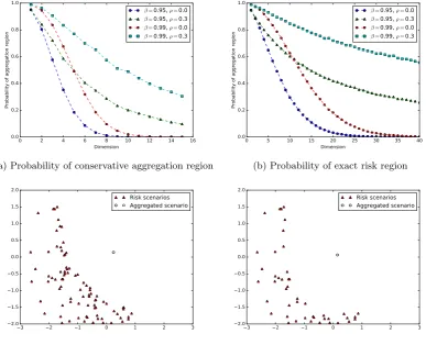
The results of this experiment are plotted in Figure 1. In Figures 1a and 1b are plotted the probabil-ities of the conservative and exact aggregation regions. To aid the readers’ intuition we have also plotted a reduced scenario set in two dimensions using conservative and exact risk regions in Figures 1c and 1d forρ= 0.3 andβ= 0.95.
of the aggregation regions for the correlated asset returns is greater and decays more slows than that of the independent asset returns. This tells us that, in addition to the loss function, the performance of our methodology depends strongly on the distribution of the random vector. Although the probability of the conservative aggregation region decays fairly rapidly, it remains non-negligible for random vectors of a moderate dimension, around 15, for the correlated asset returns. For exact aggregation regions, the probability remains high for the correlated asset returns for up to a dimension of 40.
0 2 4 6 8 10 12 14 16 Dimension
0.0 0.2 0.4 0.6 0.8 1.0
Probability of aggregation region
β=0.95, ρ=0.0
β=0.95, ρ=0.3
β=0.99, ρ=0.0
β=0.99, ρ=0.3
(a) Probability of conservative aggregation region
0 5 10 15 20 25 30 35 40 Dimension
0.0 0.2 0.4 0.6 0.8 1.0
Probability of aggregation region
β=0.95, ρ=0.0
β=0.95, ρ=0.3
β=0.99, ρ=0.0
β=0.99, ρ=0.3
(b) Probability of exact risk region
3 2 1 0 1 2 3
2.0 1.5 1.0 0.5 0.0 0.5 1.0 1.5 2.0
Risk scenarios Aggregated scenario
(c) Scenario set constructed by aggregation reduc-tion using conservative aggregareduc-tion region
3 2 1 0 1 2 3
2.0 1.5 1.0 0.5 0.0 0.5 1.0 1.5 2.0
Risk scenarios Aggregated scenario
[image:23.595.100.488.174.488.2](d) Scenario set constructed by aggregation reduc-tion using exact aggregareduc-tion region
Figure 1: Probabilities of conservative and exact aggregation regions
8.2
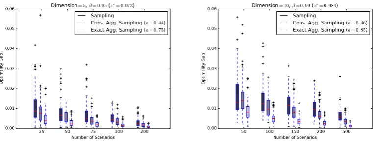
Performance of aggregation sampling
We now test the performance of the aggregation sampling algorithm using conservative and exact risk regions against standard Monte Carlo sampling in terms of the quality of the solutions each method yields.
Experimental Set-up We use the following problem:
minimize
x≥0 β-CVaR(−x
Tξ) (P)
subject to xTµ≥t
d
X
i=1
xi = 1