Higher Order Moments, Spectral and Bispectral Density Functions for INAR(1)

Higher Order Moments, Spectral and Bispectral Density

Functions for INAR(1)

M. M. Gabr

Alexandria University Department of Mathematics

Faculty of Science

B. S. El-Desouky

Mansoura University Department of Mathematics

Faculty of Science

F. A. Shiha

Mansoura University Department of Mathematics

Faculty of Science

Shimaa M. El-Hadidy

Mansoura University Department of Mathematics

Faculty of Science

ABSTRACT

In this paper, some higher order moments, spectral and bispec-tral density functions for some integer autoregressive of order one (INAR(1)) models are calculated. These models are the new skew INAR(1) (NSINAR(1)), the shifted geometric INAR(1) type-II (SGINAR(1)-type-II) and the dependent counting geometric INAR(1) (DCGINAR(1)). The spectrum, bispectrum and normalized bispec-trum are estimated using the one and two dimensional lag windows as in Subba Rao and Gabr(1984). A realization is generated for each model of size n=500 for estimation. Also, the bispectral den-sity function and normalized bispectral denden-sity function are used for studying the linearity of integer valued time series models.

Keywords

INAR(1); NSINAR(1); SGINAR(1)-II; DCGINAR(1); Moments; Cumulants; Spectrum; Bispectrum; Normalized bispectrum; Parzen lag window; 2-dimensional Subba Rao and Gabr lag window

1. INTRODUCTION

Integer valued time series used in many fields in life such as medicine, economics, etc,. . . . McKenzie (1985) introduced integer valued autoregressive (INAR) models by replacing the scalar mul-tiplication in the standard AR by thinning operator. The thinning operator defined as a probabilistic operation that can be applied to random counts when the thinning operator deletes some of these counts, the size of the shrinked counts is still integer-valued so, INAR is the best model for modelling large counting values in-stead of approximating it into continuous-valued models. The first and most popular thinning operator is the binomial thinning op-erator that introduced by Steutel and Van Harn (1979) based on the sum of Bernoulli counting series. After that, there are many types of thinning operators appears such as geometric and nega-tive binomial thinning operators, thinning operators with dependent structure, mixed thinning operator, operators acting on true integer autoregressive, etc. . . . Through the last three decades statisticians tried to made the INAR models more realistic and flexible for prac-tical purposes of modelling the observed data, thus they made some modifications on INAR. Some of them, modify the marginal distri-bution of INAR, others, modify the order of the model and others modify the thinning operators of the models. Al-Osh and Al-Zaid (1987) defined the INAR(1) based on the binomial thinning

opera-tor as

Xt=α◦Xt+εt, t∈Z,

where the operator ’◦’ is defined asα◦X =

X P

i=1

Yi,α∈ (0,1),

{Yi}is a sequence of i.i.d Bernoulli random variables with

prob-abilityα.{εt}is a sequence of i.i.d non-negative integer valued

random variables with meanµand varianceσ2_,thinning

opera-tions are performed independently of each other and of{εt}and

{Xs}s<t.The probability generating function (pgf) ofεtis given

by

Φε(s) =

ΦX(s)

ΦX(1−α+αs)

.

The first four moments ofεt using the pgf are given by

E(εt) = Φ 0 εt(1),

E(ε2 t) = Φ

0

εt(1) + Φ

00 εt(1),

E(ε3 t) = Φ

0

εt(1) + 3Φ

00

εt(1) + Φ

000 εt(1),

E(ε4 t) = Φ

0

εt(1) + 7Φ

00

εt(1) + 6Φ

000 εt(1) + Φ

0000 εt(1).

If{Xt}is stationary process to k-th order, then the k-th order joint

moment of

Xt, Xt+s1,· · · , Xt+sk−1is a function of k-1 parameters defined by

µX(s1, s2, ..., sk−1) =E(XtXt+s1...Xt+sk−1), with

µ=E(Xt).

The k-th order joint centeral moments are given by

Ck(t1, t2, ..., tk−1) = E[(Xt − µ)(Xt+t1 − µ)(Xt+t2 − µ)...(Xt+tk−1−µ)].

Leonov and Shiryaev (1959) derived relations between joint mo-ments and joint cumulants of a stationary time series

Cum(Xt) =E(Xt), (1)

C2(t1) =µ(t1)−µ

2

, (2)

Volume 182 - No.9, August 2018 order cumulants satisfy the following symmetry relations

C2(t) =C2(−t),

C3(0, t) = C3(t,0) =C3(−t,−t)

= C3(0,−t) =C3(−t,0) =C3(t, t),

C3(s, s+t) = C3(s+t, s) =C3(−s, t)

= C3(t,−s) =C3(−s−t,−t) =C3(−t,−t−s),

fors≥0andt≥0.

1.1 The spectral and bispectral density functions

The spectral density (second-order spectrum) , f(.), of{Xt}can

be expressed as the Fourier transform of autocovariance function (C2(.)),

fX(ω) =

1 2π

∞ X

t1=−∞

C2(t1) e−it1ω, −π≤ω≤π, (4)

whereP∞

t1=−∞|C2(t1)|<∞.

The bispectral and normalized bispectral density functions are given respectively as

fX(ω1, ω2) =

1 (2π)2

∞ X

t1=−∞ ∞ X

t2=−∞

C3(t1, t2)e−i(t1ω1+t2ω2),

(5)

g(ω1, ω2) =

f(ω1, ω2) p

f(ω1)f(ω2)f(ω1+ω2)

, (6)

where−π ≤ ω1, ω2 ≤ π.The bispectral density function exists

for allω1, ω2if

∞ P

t1=−∞ ∞ P

t2=−∞

|C3(t1, t2)|<∞.

The bispectral density function is a complex valued function takes the form

fX(ω1, ω2) =r(ω1, ω2) +iq(ω1, ω2).

The modulus and phase of the bispectral density function are given respectively, by

|fX(ω1, ω2)|= (r2(ω1, ω2) +q2(ω1, ω2))

1 2_,

phase=tan−1₍q(ω1, ω2)

r(ω1, ω2)

).

The bispectral density function provides us useful information about the linearity of the process. For continuous non-Gaussian time series the modulus of the normalized bispectrum is flat.

1.2 Estimation of spectrum

There are many methods for estimating the spectrum and bispec-trum, but in this paper we interested in estimating the spectrum and bispectrum using the smoothed periodogram using the Parzen lag window. The smoothed spectral and bispectral density functions are

respectively given by

ˆ

f(ω) = 1 2π

n X

s=−n

λ( s

M)e −isω_Cˆ

2(s)

= 1 2π

n X

s=−n

λ( s

M) ˆC2(s) cosωs, (7)

and

ˆ

f(ω1, ω2) =

1 4π2

N−1 X

s1=−(N−1) N−1 X

s2=−(N−1)

λ(s1

M, s2

M)

×_Cˆ_{3(s1, s2)e}−is1ω1−is2ω2_{, (8)} whereCˆ2(s),Cˆ2(s1, s2)are given by

ˆ

C2(s) =

1

N−s

N−|s| X

t=1

(X_t−X¯)(X_t+|s|−X¯),

¯

X = 1

N

N X

t=1

Xt,

ˆ

C3(s1, s2) =

1

N

N−γ X

t=1

(Xt−X¯)(Xt+s1−X¯)(Xt+s2−X¯),

wheres1, s2 ≥0, γ= max(s1, s2), s= 0,±1,±2, . . . ,±(N−

1),−π ≤ ω1, ω2 ≤ π,”λ(.)” is one-dimensional lag window

and”λ(s1

M, s2

M)” is two-dimensional lag window [Parzen, Daniell,

Tukey Hamming ,...]. In this paper, we use the Parzen lag window. Parzen (1961b) proposed the Parzen lag window

λ(s) =







1−6s2_{+ 6|s|}3

2(1− |s|)3

0

|s| ≤1 2 1

2 <|s| ≤1

|s|>1

, (9)

andλ(s1, s2)is given by

λ(s1, s2) =λ(s1)λ(s2)λ(s1−s2). (10)

The normalized bispectrum is estimated by

ˆ

g(ω1, ω2) =

ˆ

f(ω1, ω2) q

ˆ

f(ω1) ˆf(ω2) ˆf(ω1+ω2)

. (11)

for more details about the estimation of spectrum and lag windows, see [16]

This paper is organized as follows. In Section 2, some higher order joint moments of the NSINAR(1) model up to order three, the spec-tral and bispecspec-tral and normalized bispecspec-tral density functions are calculated. Moreover, the estimates for the spectral, bispectral and normalized bispectral density functions using a simulated realiza-tion of size n=500 are calculated. Also, the linearity of the model is investigated. In Section 3, the same measures are calculated for the SGINAR(1)-II model. In Section 4, the same measures are cal-culated for the DCGINAR(1) model.

2. THE NEW SKEW INAR(1) MODEL

as the difference between Poisson INAR(1) model that introduced by Al-Osh and Al-Zaid (1987) and the NGINAR(1) model that in-troduced by Risti`c et al.(2009) see [1] and [11]. They defined the NSINAR(1) model as

Zt=α ? Zt−1+ζt, (12)

whereα ? Zt−1 d

=α∗Xt−1−α◦Yt−1is the difference between the

negative binomial thinning and binomial thinning operators, where the counting seriesα∗Xt−1andα◦Yt−1are independent random

variables.α∗X =

X P

i=0

Wi and α◦Y = Y P

i=0

Ui,where{Wi}

is a sequence of i.i.d geometric random variables and{Ui}is a

sequence of i.i.d Bernoulli random variables independent of{Wi}

,Zt =Xt−YtwhereXt ∼geometric (₁₊µ_µ),Yt ∼Poisson(λ),

{Zt}be a sequence of random variables has a Geometric-Poisson

(µ, λ) andζthas the distribution oft−εt,where{t}and{εt}

are independent r.v’s and Ztandζt−lare independent for alll≥1.

{εt}are i.i.d r.v’s with common poisson(λ(1−α)) distribution and

t is a mixture of two random variables with geometric (µ/(1 +

µ)) and geometric (α/(1 +α)) distributions. The condition of the stationarity of the process{Zt}is0≤ α ≤ µ/(1 +µ)and the

condition of the non-stationarity of the process{Zt}isµ/(1+µ)≤

α≤1.Here, our study is restricted to the stationary case. The moment generating function ofζt andZt are given,

respec-tively, by (see [5])

Mζ(s) =

[1 +α(1 +µ)(1−es_)]e[λ(1−α)(e−s_−1)]

[1 +µ(1−es_{)][1 +α(1−e}s_)] ,

MZ(s) =

eλ(e−s₋₁₎

[1 +µ(1−es_)].

The mean and variance ofZtandζtare then given by

µZ = µ−λ, σ2Z=µ 2

+µ+λ, µζ = (1−α)[µ−λ],

σ2

ζ = (1 +α)µ[(1−α)(1 +µ)−α] +λ(1−α).

The thinning operator has the following properties (1) E(α ? Z) =α(µ−λ).

(2) E(α ? Z)2_=α2_(µ−λ)2_{+αµ(1 + 2α+αµ) +αλ.}

(3) E(α ? Z)2_=α2_E(Z2_{) +α(1 +α)E(X) +α(1−α)E(Y)}

=α2_E(Z2_)−α2_{E(Z) +α(µ+λ).}

2.1 The higher order joint central moments (cumulants)

THEOREM 1. Let{Zt}be a stationary process satisfying (12)

then,

the second- order central moment is calculated as C2(s) =αs(µ2+µ+λ) =αsC2(0).

The third- order central moment are calculated as C3(0,0) = 2µ3+ 3µ2+µ−λ,

C3(0, s) =αs(2µ3+ 3µ2+µ−λ) =αsC3(0,0),

C3(s, s) =α2sC3(0,0)−αC2(0)α

s_−α2s

(1−α) .

PROOF. µ(s)is calculated as

µ(s)=E(ZtZt+s) =E(Zt(α ? Zt+s−1+ζt))

=αµ(s−1)+µZµζt=α

s_µ

(0)+1−α

s

1−αµZµζt

=αs_[2µ2_+µ+λ2_{+λ−2µλ] + (1−α}s_)(µ−λ)2

=αs_[µ2_{+µ+λ] + (µ−λ)}2_,

then,C2(s)is calculated as

C2(s) =µ(s)−µ2Z.

C3(0,0)is calculated as

C3(0,0) =µ(0,0)−3µZµ(0)+ 2µ3Z.

µ(s,s)is calculated as

µ(s,s)=E(ZtZt+sZt+s) =E(Zt[α ? Zt+s−1+ζt]2)

=α2_E(Z

tZt+s−1Zt+s−1)−α2E(ZtZt+s−1)+α(µ+λ)E(Zt)+

2αE(ZtZt+s−1)E(ζt) +E(ζt2)E(Zt)

=α2_µ

(s−1,s−1)+[2αµζ−α2]µ(s−1)+α(µ+λ)µZ+µZ[σ2ζ+µ 2 ζ]

=α2_µ

(s−1,s−1)+[2αµζ−α2][µ2+µ+λ]αs−1+(µ−λ)2[2αµζ−

α2_{] +α(µ+λ)µ}

Z+µZ[σζ2+µ 2 ζ]

=α2s_µ

(0,0)+ [2αµζ−α2][µ2+µ+λ] Ps−1

i=0αs

−(i+1)_α2i_{+ [(µ−}

λ)2_[2αµ

ζ−α2] +α(µ+λ)µZ+µZ[σ2ζ+µ2ζ]] Ps−1

j=0α 2j

=α2s_µ

(0,0)+([2αµζ−α2][µ2+µ+λ])α

s−α2s

α(1−α)+[(µ−λ) 2_[2αµ

ζ−

α2_{] +α(µ+λ)µ}

Z+µZ[σζ2+µ 2 ζ]]

1−α2s 1−α2, then,C3(s, s)is calculated as

C3(s, s) =µ(s,s)−µ[E(Zt2+s) + 2µ(s)] + 2µ3

=α2_µ

(s−1,s−1)−α2µ(s−1)+α(µ+λ)µZ+2αµ(s−1)µζ+µZ[σ2ζ+

µ2

ζ]−2µZ[αµ(s−1)+µZµζt]−µZE((α ? Zt+s−1+ζt)

2_{) + 2µ}3

=α2_µ

(s−1,s−1)−α2µ(s−1)+α(µ+λ)µZ+2αµ(s−1)µζ+µZ[σ2ζ+

µ2

ζ]−2µZ[αµ(s−1)+µZµζt]−µZ[E(α ? Zt+s−1)

2_+E(ζ t2) +

2αE(ζt)E(Zt+s−1) + 2µ3 =

α2_µ

(s−1,s−1)−α2µ(s−1)+α(µ+λ)µZ+ 2αµ(s−1)µζ+µZ[σ2ζ+

µ2

ζ]− 2µZ[αµ(s−1) + µZµζt] − µZ[σ

2 ζ + µ

2

ζ] − 2αµ 2 Zµζ −

µZ[α2E(Zt2+s−1)−α2E(Zt+s−1) +α(µ+λ)] + 2µ3

= α2_[µ

(s−1,s−1) − µZE(Zt2+s−1) − 2µZµ(s−1) + 2µ3] −

α2_[µ

(s−1)−µ2Z] =α 2_C

3(s−1, s−1)−α2C2(s−1)

=α2_C

3(s−1, s−1)−α2αs−1C2(0)

=α2s_C

3(0,0)−α2C2(0) Ps−1

i=0α

s−(i+1)_α2i _=α2s_C 3(0,0)−

α2_C 2(0)α

s_−α2s

α(1−α).

µ(0,s)is calculated as

µ(0,s)=E(ZtZtZt+s) =E(ZtZt[α ? Zt+s−1+ζt])

=αE(ZtZtZt+s−1) +E(Zt2)E(ζt) =αµ(0,s−1)+ [2µ2+µ+

λ2_{+λ−2µλ][(1−α)(µ−λ)]}

=αs_µ

(0,0)+1−α

s

1−α[2µ

2_+µ+λ2_{+λ−2µλ][(1−α)(µ−λ)]}

=αs_[6µ3_−6λµ2_{+ 6µ}2_{+ 3µλ}2_−3λ2_−λ3_{−λ+µ] + (1−}

αs_{)(µ−λ)[2µ}2_+µ+λ2_{+λ−2µλ].}

ThenC3(0, s)is calculated as

C3(0, s) =µ(0,s)−µZ[µ(0)+ 2µ(s)] + 2µ3

= (µ−λ)[2µ2_+µ+λ2_{+λ−2µλ] +α}s_{µ[1 + 5µ−2λµ+ 4µ}2_]−

αs_{λ[1 + 2λ]−(µ−λ)[2µ}2_+µ+λ2_{+λ−2µλ+ 2(α}s_[µ2_+µ+

λ] + (µ−λ)2_{)] + 2(µ−λ)}3_.

µ(s,τ)is calculated as

µ(s,τ)=ατ−sµ(s,s)+(1−ατ−s)[αs[µ2+µ+λ]+(µ−λ)2][µ−λ].

µ(0) andµ(0,0)are given by Bourguignon and Vasconcellos (see

[5]).

2.2 The spectral, bispectral and normalized bispctral density functions of the NSINAR(1)

The spectral density function is given by (see [5])

fZ(ω) =

(1−α2_)(µ2_+µ+λ)

Volume 182 - No.9, August 2018 THEOREM 2. The bispectral density function is calculated as

fZ(ω1, ω2) =

1

(2π)2[C3(0,0) +C3(0,0){h1(−ω1) +h1(−ω2)

+h1(ω1+ω2)}+ (C3(0,0) +

α2_C 2(0)

α(1−α)){h2(ω1) +h2(ω2) +h2(−ω1−ω2)}

−α

2_C 2(0)

α(1−α){h1(ω1) +h1(ω2) +h1(−ω1−ω2)} +(C3(0,0) +

α2_C 2(0)

α(1−α)){h2(−ω1−ω2)h1(−ω2) +h2(−ω1−ω2)h1(−ω1) +h2(ω2)h1(−ω1)

+h2(ω1)h1(−ω2) +h2(ω1)h1(ω1+ω2)

+h2(ω2)h1(ω1+ω2)}

−α

2_C 2(0)

α(1−α){h1(−ω1−ω2)h1(−ω2) +h1(−ω1−ω2)h1(−ω1) +h1(ω2)h1(−ω1)

+h1(ω1)h1(−ω2) +h1(ω1)h1(ω1+ω2)

+h1(ω2)h1(ω1+ω2)}], (14)

whereh1(ωk) = αe

iωk

1−αeiωk andh2(ωk) = α2_eiωk

1−α2_eiωk,k=1,2.

PROOF. The proof is too long to included it here.

The normalized bispectral density function is calculated by(6),

wherefZ(ω)and fZ(ω1, ω2) are respectively given by (13) and

(14) .

2.3 Estimation of spectrum

Estimates of the spectral, bispectral and normalized bispectral density functions are calculated using the smoothed periodogram method using Parzen lag window and simulated series from the NSINAR(1) model.

The theoretical spectrumfZ(ω), theoretical bispectral and

normal-ized bispectral modulus offZ(ω1, ω2)andgZ(ω1, ω2)are

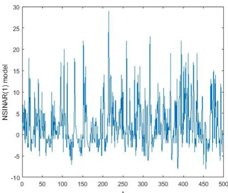
respec-tively computed by settingα =.25, µ = 5and λ= 3in (13), (14) and (6). Fig. 1 represent the simulated series of {Zt, t =

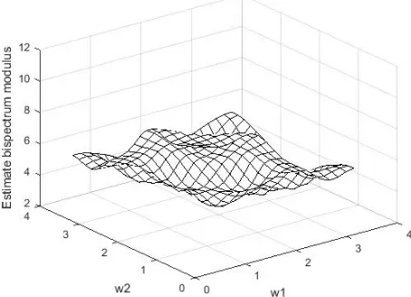
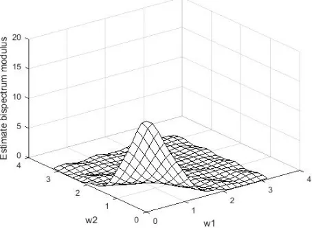
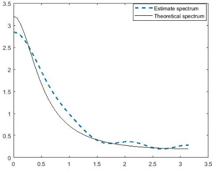
1, ...,500}from the NSINAR(1) model withα=.25, λ= 3and µ= 5that defined by (12). Fig. 2 represent theoretical spectrum and the estimate of the spectral density using Parzen window with M=7 as in (7) and (9). Fig. 3 and Fig. 4 represent the theoretical bispectrum and normalized bispectrum modulus. Fig. 5 and Fig. 6 represent the estimate of the bispectrum and normalized bispectrum modulus with M=7 by Parzen window using (8), (10) and (9).

List of Tables

1 Theoretical bispectral modulus of NSINAR(1) with α=.25, λ= 3andµ= 5. . . 12 2 Theoretical normalized bispectral modulus of

[image:4.595.320.544.76.265.2]

NSI-NAR(1) withα=.25, λ= 3andµ= 5. . . 12 It is clear that the values of the normalized bispectrum modulus given in Table 2 show that the normalized bispectrum modulus of the NSINAR(1) model is more flat than the non-normalized one given in Table 1.This indicates that the test of linearity given by Subba Rao and Gabr (1980) and its modification given by Hinich (1982) can be used for integer valued time series models.

[image:4.595.328.545.309.487.2]

Fig. 1. Simulated series of NSINAR(1) model withα=.25, λ= 3and µ= 5.

Fig. 2. The theoretical spectrum is represented by a solid line and esti-mated spectrum is represented by a dash line.

Fig. 3. Theoretical bispectral modulus of the NSINAR(1) withα =

[image:4.595.321.547.536.706.2]

[image:5.595.48.285.79.250.2] [image:5.595.57.284.305.469.2]

Fig. 4. Theoretical normalized bispectral modulus of NSINAR(1) with α=.25, λ= 3andµ= 5.

Fig. 5. Estimate bispectral modulus of NSINAR(1) at M=7.

Fig. 6. Estimate normalized bispectral modulus of NSINAR(1) at M=7.

3. THE SHIFTED GEOMETRIC INAR(1) MODEL(

SGINAR(1)-II)

Shifted geometric INAR(1) of type-II (in short, SGINAR(1)-II model introduced by Nasti´c (2012). It has the same approach that taken by Bakouch and Risti´c (2010) for ZTPINAR(1) process but SGINAR(1)-II model is based on negative binomial thinning op-erator. A process{Xt}is said to be SGINAR(1)-II if it satisfies

Xt=

ηt with probability₁₊1_µ

α∗Xt−1+ηt with probability1+µµ

, (15)

where the operator ”∗” is defined as

α∗Xt−1= Xt−1

X

i=1

Yi, α∈(0,1),

where{Yi}is a sequence of i.i.d random variables with

geomet-ric ( 1

1+α) distribution independent ofXt−1,{Xt}is a stationary

process has shifted geometric (₁₊1_µ) distribution and{ηt}are i.i.d

random variables independent ofYiand ofXt−i, i≥1.The pgf of

Xtandηtare given by respectively (see[9])

φX(s) =1+µs−µs,

φη(s) =1+α1−αs

_α(1+µ)

µ s+

µ−α(1+µ) µ

s 1+µ−µs

.

The mean and variance ofXt andηtare then given by respectively

µX = 1 +µ, σX2 =µ(1 +µ),

µηt = (1 +µ−αµ), σ

2

ηt=µ(1−α+µ−α

2_µ−2α2_).

For more information about the model and the binomial thinning operator see [9] and [11].

3.1 Higher order joint moments and cumulants

THEOREM 3. Let{Xt}be a stationary process satisfying (15)

then,

The first order moment and cumulant for SGINAR(1)-II are given by µX.

The second order joint moments are calculated as µ(0)= (1 +µ)(1 + 2µ),

µ(s)=µ(µ+ 1)

α_µµ₊₁

s

+ (1 +µ)2_.

Then, the second order joint central moment is calculated as C2(s) = [1+αµµ]

s_C

2(0) = (1+αµµ)

s_{µ(µ+ 1).}

The third order joint moments are calculated as µ(0,0)= 6µ3+ 12µ2+ 7µ+ 1,

µ(0,s)= (₁₊αµ_µ)s(4µ2+ 3µ) (µ+ 1) + (µ+ 1) (3µ+ 2µ2+ 1),

µ(s,s) = {(αµµ+1)

s_(2µ2 _{+ 3µ − 2αµ}2 _{+ αµ)(}µ+1 1−α) +

(α2 µ µ+1)

s_(2µ2_{−4αµ−2αµ}2₎₍µ+1 1−α) + (

µ+1

1−α)(1−2αµ

2_{+ 2µ}2₋

3αµ+ 3µ−α),

µ(s,τ)= (₁₊αµ_µ)τ−s(µ(s,s)−µ(s)µX) +µ(s)µX.

Then, the third order joint central moments are calculated as

C3(0,0) = (1 +µ)µ(1 + 2µ) =µ(2µ2+ 3µ+ 1),

C3(0, s) = (₁₊αµ_µ)sC3(0,0) = (₁₊αµ_µ)sµ(2µ2+ 3µ+ 1),

C3(s, s) = (α

2_µ

1+µ) s_C

3(0,0) + [1+αµµ(1 +α) + 2(1 +µ)[ α2_µ

1+µ−

( αµ 1+µ)

2_]]C 2(0)

(₁₊αµ_µ)s−(α₁₊2µ_µ)s

αµ

1+µ− α2µ

1+µ

=

α2 µ µ+1

s

(2µ − 4α − 2αµ)µ(µ₁₋+1_α) +

α_µµ₊₁

s

(3α +

[image:5.595.57.284.513.684.2]

Volume 182 - No.9, August 2018 C3(s, τ) = (1+αµµ)

τ−s_C 3(s, s).

The fourth-joint moments are calculated as µ(0,0,s)=1+αµµµ(0,0,s−1)+µηµ(0,0), s >0,

µ(0,s,τ)= αµ

1+µµ(0,s,τ−1)+µ(0,s)µη, τ > s >0,

µ(0,s,s) = α

2_µ

1+µµ(0,s−1,s−1) + αµ

1+µ(1 + α)µ(0,s−1) +

2₁₊αµ_µµηµ(0,s−1)+ (1 + 3µ−3αµ−2µα2+ 2µ2−2αµ2)(1 +

3µ+ 2µ2_),

µ(s,τ,u)= ₁₊αµ_µµ(s,τ,u−1)+µηµ(s,τ), u > τ > s >0,

µ(s,s,v) = ₁₊αµ_µµ(s,s,v−1) + µηµ(s,s), v > s > 0,

µ(s, s, s) =₁₊α3µ_µµ(s−1,s−1,s−1)+3α

2_µ

1+µ[(1+α)+µη]µ(s−1,s−1)+ αµ

1+µ[(1 +α)(1 + 2α) + 3µη(1 +α) + 3(1 + 3µ−3αµ−2µα2+

2µ2_−2αµ2_)]µ

(s−1)+ (1 +µ)(1 + 7µ−7αµ−12µα2+ 12µ2−

12αµ2_−6α3_µ−6α2_µ2_{+ 6µ}3_−6µ3_α).

Then, the fourth order joint cumulants are calculated as C4(0,0, s) = ₁₊αµ_µC4(0,0, s−1), s≥0,

C4(0, s, s) = α

2_µ

1+µC4(0, s−1, s−1) + αµ

1+µ(1 +α)C3(0, s−1),

s≥0,

C4(0, s, u) = 1+αµµC4(0, s, u−1), u≥s≥0,

C4(s, τ, u) = 1+αµµC4(s, τ, u−1), u≥τ≥s≥0,

C4(s, s, s) =α

3_µ

1+µC4(s−1, s−1, s−1) + 3α

2_µ

1+µ(1 +α)C3(s−

1, s−1) + αµ

1+µ(1 +α)(1 + 2α),

C4(s, s, u) =1+αµµC4(s, s, u−1), u≥s≥0.

PROOF. The proof of this theorem is similarly to the proof of theorem 1 in section 2, by using the definition of the SGINAR(1)-II and higher order moments and cumulants and the properties of the negative binomial thinning operator.

3.2 The spectral, bispectral and normalized bispectral density functions

The spectral density function is given by Nasti´c (2012) (see[9])

fX(ω) =

µ(1 +µ)(1 + 2µ+ 2µ2_(1−α2₎₎

2π(1 + 2µ+µ2_{(1 +α}2_{)−2αµ(1 +µ) cosω)}.

(16) The normalized spectral density function is calculated as

gX(ω) =

(1 + 2µ+ 2µ2_(1−α2₎₎

2π(1 + 2µ+µ2_{(1 +α}2_{)−2αµ(1 +µ) cosω)}.

THEOREM 4. The bispectral density function is calculated as

fX(ω1, ω2) =

1

(2π)2[C3(0,0) +C3(0,0){H1(−ω1)

+H1(−ω2) +H1(ω1+ω2)}+ (C3(0,0)

−[(1 +α) + 2(1 +µ)α(1−

µ

1+µ)]C2(0)

1−α )

{H2(ω1) +H2(ω2) +H2(−ω1−ω2)}

+[(1 +α) + 2(1 +µ)α(1−

µ

1+µ)]C2(0)

1−α

{H1(ω1) +H1(ω2) +H1(−ω1−ω2)}

+(C3(0,0)

−[(1 +α) + 2(1 +µ)α(1−

µ

1+µ)]C2(0)

1−α )

{H1(−ω2)H2(−ω1−ω2)

+H1(−ω1)H2(−ω1−ω2)

+H1(−ω2)H2(ω1) +H1(−ω1)H2(ω2)

+H1(ω1+ω2)H2(ω1) +H1(ω1+ω2)H2(ω2)}

+[(1 +α) + 2(1 +µ)α(1−

µ

1+µ)]C2(0)

1−α {H1(−ω2)H1(−ω1−ω2)

+H1(−ω1)H1(−ω1−ω2)

+H1(−ω2)H1(ω1) +H1(−ω1)H1(ω2)

+H1(ω1+ω2)H1(ω1)

+H1(ω1+ω2)H1(ω2)}], (17)

whereH1(ωk) =

αµ

1+µeiωk

1−₁₊αµ_µeiωk andH2(ωk) =

α2µ

1+µeiωk

1−α₁₊2µ_µeiωk

withk= 1,2.

PROOF. The proof is too long to included it here.

The normalized bispectral density function is calculated as (6), wherefX(ω1, ω2)andfX(ω1)are defined in (17) and (16).

3.3 Estimation of spectrum

The estimates of the spectral, bispectral and normalized bispectral density functions are calculated using the smoothed periodogram method based on the Parzen lag window using simulated series {Xt, t= 1,2, . . . ,500}from SGINAR(1)-II model.

The theoretical spectrumfX(ω),theoretical bispectral and

normal-ized bispectral modulus offX(ω1, ω2)andgX(ω1, ω2)are

respec-tively computed by settingµ= 2.6andα=.6in (17) and (6). Fig. 7 represents the simulated series of SGINAR(1)-II withµ= 2.6 andα = .6. Fig. 8 represents theoretical spectrum and the esti-mate spectrum by Parzen window with M=7 as in (7) and (9). Fig. 9 and Fig. 10 represent the theoretical bispectrum and normalized bispectrum modulus. Fig. 11 and Fig. 12 represent the estimate of the bispectrum and normalized bispectrum modulus with M=7 by Parzen window using (8), (11) and (10).

[image:7.595.60.281.75.255.2] [image:7.595.316.548.80.250.2]

Fig. 7. Simulated series of SGINAR(1)-II withµ= 2.6andα=.6.

Fig. 8. Theoretical spectrum is represented by a solid line and estimated spectrum is represented by a dash line at M=7.

Fig. 9. The theoretical bispectral modulus of SGINAR(1)-II withµ= 2.6

[image:7.595.65.284.288.463.2]

andα=.6.

Fig. 10. The theoretical normalized bispectral modulus of SGINAR(1)-II withµ= 2.6andα=.6.

Fig. 11. Estimate bispectral modulus of SGINAR(1) at M=7.

[image:7.595.321.548.304.470.2] [image:7.595.57.283.513.684.2] [image:7.595.317.550.513.682.2]

Volume 182 - No.9, August 2018

4. THE DEPENDENT COUNTING GEOMETRIC

INAR(1) MODEL

Risti´c et al. (2013) introduced the DCGINAR(1) model based on generalized binomial thinning operator type-I with a geometric marginal (•θ). They defined the DCGINAR(1) as

Xt=α•θXt−1+εt, t∈Z, α, θ∈(0,1), (18)

where the operator ’•θ’ is defined asα•θX = PX

i=1Ui,i∈N,

{Ui}is a sequence of dependent Bernoulli(α) random variable

de-fined asUi= (1−Vi)Wi+ViZ,{Wi}is a sequence of i.i.d

ran-dom variable with Bernoulli(α) distribution,{Vi}is a sequence of

i.i.d random variable with Bernoulli(θ) distribution,Zis a random variable with Bernoulli(α) distribution,Wi, VjandZare

indepen-dent∀i, j∈Nand{Ui}are independent ofXlandεmfor anyi, l

andm.{Xt}has Geometric (₁₊µ_µ) distribution,µ >0and{εt}is a

sequence i.i.d r.v’s distributed as a mixture of zero and two geomet-rically random variables. This model satisfy these conditions,{εt}

is a sequence i.i.d random variables such thatCov(εt, Xs) = 0,

s < t.,{Ui}are independent ofXjandεkand{Ui}used for

gen-eratingXsandXt, representing the counting series of the process

{Xt}are mutually independent fort6=s.

The pgf ofUi,εtandXtare given by respectively (see[12])

φUi(s) = 1−α+αs,

φε(s) =(1+α(1

−θ)µ−α(1−θ)µs)(1+(α+θ−αθ)µ−(α+θ−αθ)µs) (1+µ−µs)(1+(α+θ−2αθ)µ−(α+θ−2αθ)µs) ,

φX(s) =1+µ1−µs.

The mean and variance ofXtandεtare respectively given by

µX=µ, σ2X=µ(1 +µ),

µεt = (1−α)µ, σ

2

εt= (1−α)µ(1 + (1 +α−2αθ

2_)µ).

The second and third moments ofεtare respectively calculated as

E(ε2_{) = (1−α)µ+ 2(α−1)(αθ}2_−1)µ2_{, (19)}

E(ε3) = (1−α)µ+ 6(α−1)(αθ2−1)µ2 −6(α−1)(−α2_θ2

+2α2θ3−αθ3−αθ2+ 1)µ3. (20) Some properties of the operator ’•θ

’:-LetX, Y be any two random variables with finite first, second and third moments,α∈(0,1)andθ∈(0,1),then

(1) E(α•θX) =αE(X),

(2) E(α•θX)2 =α(α+ (1−α)θ2)E(X2) +α(1−α)(1−

θ2_)E(X)

(3) E(Y(α•θX)) =αE(XY).

(4) E(α•θX)3 = [α3−3α2θ3+ 2α3θ3−3α3θ2+ 3α2θ2+

αθ3_]E(X3_{) + [9α}3_θ2_−6α3_θ3_−12α2_θ2_−3αθ3_{+ 3αθ}2₊

3α2_+9α2_θ3_−3α3_]E(X2_)+[9α2_θ2_−3α2_−6α2_θ3_−6α3_θ2₋

3αθ2_{+α+ 2α}3_{+ 2αθ}3_{+ 4α}3_θ3_]E(X).

For more details about the model and the properties of the general-ized binomial thinning type-I see [12].

4.1 Higher order joint moments and cumulants

THEOREM 5. Let{Xt}be a stationary process satisfying (18)

then,

The first-order moment and first cumulant are given byµX.

The second-order joint moment is calculated as

µ(s)=αs[µ(0)−µ2] +µ2=αsµ(1 +µ) +µ2, s≥0and

µ(0)=µ(1+2µ).

Then, the second order joint central moment is calculated as C2(s) =αsC2(0) =αsµ(1 +µ), s≥0.

The third-order moments are calculated as µ(0,0)=µ(1 + 6µ+ 6µ2),

µ(0,s) =αs[µ(0,0)−µµ(0)] +µµ(0)=µ2(1 + 2µ) +αsµ(1 +

5µ+ 4µ2_{), s≥0,}

µ(s,s) = [α(α+ (1−α)θ2)]sµ(0,0) + [α(1−α)(1−θ2) +

2αµε](µ(0)−µ2)[α

s_{−(α(α+(1−α)θ}2₎₎s

α(1−[α(α+(1−α)θ2_)]] + ([α(1−α)(1−θ2) +

2αµε]µ2+µ[µ2ε+σ 2 ε])[

1−[α(α+(1−α)θ2_)]s

1−[α(α+(1−α)θ2)]],

µ(s,τ)=ατ−s(µ(s,s)−µ(s)µ) +µ(s)µ, τ > s.

Then, the third-order joint central moments are calculated as C3(0,0) =µ(1 + 3µ+ 2µ2),

C3(0, u) =αuC3(0,0) =αuµ(1 + 3µ+ 2µ2), u≥0,

C3(s, s) = [α(α+ (1−α)θ2)]sC3(0,0) + [α(1−α)(1−θ2) +

2µα(1−α)θ2_]C 2(0)[α

s_{(1−(α(α+(1−α)θ}2₎₎s₎

α(1−[α(α+(1−α)θ2_)]) ], s≥0, C(s, τ) =ατ−s_C

3(s, s).

The fourth-order moments are calculated as µ(0,0,s)=αµ(0,0,s−1)+µ(0,0)µε,

µ(0,s,s)=α(α+ (1−α)θ2)µ(0,s−1,s−1)+ (2α(1−α)µ+α(1−

α)(1−θ2_))µ

(0,s−1)+µ(0)(E(ε2)),

µ(0,s,τ)=αµ(0,s,τ−1)+µ(0,s)µε,

µ(s,τ,υ)=αµ(s,τ,υ−1)+µ(s,τ)µε,

µ(s,s,s) = [α3 − 3α2θ3 + 2α3θ3 − 3α3θ2 + 3α2θ2 +

αθ3_]µ

(s−1,s−1,s−1)+ [9α3θ2−6α3θ3−12α2θ2−3αθ3+ 3αθ2+

3α2_+9α2_θ3_−3α3_]µ

(s−1,s−1)+[9α2θ2−3α2−6α2θ3−6α3θ2−

3αθ2_{+α+ 2α}3_{+ 2αθ}3_{+ 4α}3_θ3_]µ

(s−1)+µE(ε3) + 3µε[α(α+

(1−α)θ2_)µ

(s−1,s−1)+α(1−α)(1−θ2)µ(s−1)]+3αE(ε2)µ(s−1),

whereE(ε2_)andE(ε3_{)are given by (19) and (20) respectively.}

The fourth-order joint cumulants are calculated as

C4(v, v, v) = [α3−3α2θ3+2α3θ3−3α3θ2+3α2θ2+αθ3]C4(v−

1, v−1, v−1) + [9α3_θ2_−6α3_θ3_−12α2_θ2_−3αθ3_{+ 3αθ}2₊

3α2_{+ 9α}2_θ3_−3α3_]C

3(v−1, v−1) + [9α2θ2−3α2−6α2θ3−

6α3_θ2_−3αθ2_{+α+ 2α}3_{+ 2αθ}3_{+ 4α}3_θ3_]C

2(v−1),

C4(0, v, v) =α(α+ (1−α)θ2)C4(0, v−1, v−1) +α(1−α)(1−

θ2_)C

4(0, v−1),

C4(0, τ, v) =αC4(0, τ, v−1), v≥τ≥0,

C4(τ, τ, s) =αC4(τ, τ, s−1), s≥τ ≥0,

C4(s, τ, v) =αC4(s, τ, v−1), v≥τ≥s≥0.

PROOF. The proof is similar to the proof of theorem 1 using the definitions of the DCGINAR(1) and the properties of the general-ized thinning operator.

4.2 The spectral, bispectral and normalized bispectral density functions

The non-normalized spectral density function fX(ω) of

DCGI-NAR(1) is calculated as

fX(ω) =

µ(1 +µ)(1−α2₎

2π(1 +α2_−2αcosω), −π≤ω≤π. (21)

The normalized spectral density functiongX(ω)is calculated as

gX(ω) =

(1−α2₎

THEOREM 6. The bispectral density functionfX(ω1, ω2) of

DCGINAR(1) is calculated as fX(ω1, ω2) =

1

(2π)2[C3(0,0){1 +F1(−ω1) +F1(−ω2)

+F1(ω1+ω2)}

+(C3(0,0)

−[(1−α)(1−θ

2_{) + 2µ(1−α)θ}2_]C 2(0)

(1−α(α+ (1−α)θ2₎₎ )

{F2(ω1) +F2(ω2) +F2(−ω1−ω2)}

+([(1−α)(1−θ

2_{) + 2µ(1−α)θ}2_]C 2(0)

(1−α(α+ (1−α)θ2₎₎ ){F1(ω1)

+F1(ω2) +F1(−ω1−ω2)}

+(C3(0,0)

−[(1−α)(1−θ

2_{) + 2µ(1−α)θ}2_]C 2(0)

(1−α(α+ (1−α)θ2₎₎ )

{F2(−ω1−ω2)F1(−ω2) +F2(−ω1−ω2)F1(−ω1)

+F2(ω1)F1(−ω2) +F2(ω2)F1(−ω1)

+F2(ω1)F1(ω1+ω2) +F2(ω2)F1(ω1+ω2)}

+([(1−α)(1−θ

2_{) + 2µ(1−α)θ}2_]C 2(0)

(1−α(α+ (1−α)θ2₎₎ )

{F1(−ω1−ω2)F1(−ω2) +F1(−ω1−ω2)F1(−ω1)

+F1(ω1)F1(−ω2) +F1(ω2)F1(−ω1)

+F1(ω1)F1(ω1+ω2) +F1(ω2)F1(ω1+ω2)}],(22)

whereF1(ωk) = αe

iωk

1−αeiωk and

F2(ωk) = α(α+(1

−α)θ2_)eiωk

1−(α(α+(1−α)θ2))eiωk,withk= 1,2.

PROOF. The proof is too long to be included here.

The normalized bispectral density function is calculated by(6),

wherefX(ω1, ω2)andf(ωi)are given by (22) and (21).

NOTATION 7. The higher order moments, cumulants , spec-trum, bispectrum and normalized bispectrum for the GINAR(1) model that introduced by Al-Zaid and Al-Osh (1988) can be con-cluded by settingθ = 0in the higher order moments, cumulants, spectrum, bispectrum and normalized bispectrum of the DCGI-NAR(1).

4.3 Estimation of the spectrum

Estimates of the spectrum, the bispectrum and normalized bis-pectrum using the smoothed periodogram method using the Parzen window and simulated series from the DCGINAR(1) model are cal-culated.

The theoretical spectrumfX(ω), theoretical bispectral and

normal-ized bispectral density offX(ω1, ω2)andgX(ω1, ω2)are

respec-tively obtained by settingα=.6, θ=.7andµ= 1.8in (21), (22) and (6). Fig. 13, represents the simulated series of DCGINAR(1) withα=.6, θ=.7andµ= 1.8. Fig. 14 represents the theoretical spectrum and the estimate spectrum using Parzen lag window with M=7 from (7) and (9). Fig. 15 and Fig. 16 represent the theoretical bispectral and normalized bispectral modulus. Fig. 17 and Fig. 18 represent the estimate of the bispectrum and normalized bispectrum modulus with M=7 by Parzen window using (8), (10) and (9). From Fig. 15 and Fig. 16, the normalized bispectrum modulus of the DCGINAR(1) is more flat than the non-normalized bispectrum modulus, since the the values of the normalized bispectrum

[image:9.595.321.544.76.254.2]

modu-Fig. 13. Simulated series of DCGINAR(1) withα = .6, θ = .7and µ= 1.8.

[image:9.595.328.543.299.476.2]

Fig. 14. Theoretical spectrum and estimated spectrum at M=7.

[image:9.595.323.549.514.682.2]

[image:10.595.56.283.78.250.2]

Volume 182 - No.9, August 2018

Fig. 16. Theoretical normalized bispectral modulus withα=.6, θ=.7

[image:10.595.60.284.305.470.2]

andµ= 1.8of DCGINAR(1).

Fig. 17. Estimate bispectral modulus of DCGINAR(1) at M=7.

Fig. 18. Estimate normalized bispectral modulus of DCGINAR(1) at M=7.

lus lies between (0.5,2) and the values of the non-normalized bis-pectrum modulus lies between (0,12).

5. CONCLUSIONS

Bispectrum and normalized bispectrum are used for checking the linearity of the models. The higher order moments, spec-trum, bispectrum and normalized bispectrum of the NSINAR(1), SGINAR(1)-II and DCGINAR(1) models are computed. The spec-trum, bispectrum and normalized bispectrum are estimated using a smoothed periodogram based on the Parzen lag window and us-ing a simulated series from each model. Moreover, the higher or-der moments, spectrum and bispectrum for the GINAR(1) are con-cluded as a special case of the DCGINAR(1) model. The normal-ized bispectrum modulus of these models are more flat than the non-normalized bispectrum modulus, so the test of linearity that given by Subba Rao and Gabr (1980) and its modification given by Hinich (1982) can be used for integer valued time series models.

6. REFERENCES

[1] Al-Osh, M. A. and Alzaid, A. A. (1987). First-order integer-valued autoregressive (INAR(1)) process.J. Time Ser. Anal.8, 261–275.

[2] Al-Zaid, A. A. and Al-Osh, M. A. (1988) First-order integer-valued autoregressive (INAR(1)) process. Distributional and Regression Properties.Statistica Neerlandica.42, 53–61. [3] Bakouch, H. S. (2010). Higher-order moments, cumulants

and spectral densities of the NGINAR(1) process.Statistical Methodology. 7,20, 1- 21.

[4] Bakouch, H. S. and Risti´c, M. M. (2010). Zero Truncated Pois-son Integer Valued AR(1) Model. Metrika 72(2), 265-280. [5] Bourguignon, M. and Vasconcellos, K. L. P. (2016). A new

skew integerb valued time series process.Statistical Method-ology31,8-19.

[6] Hinich, M. (1982). Testing for Gaussianity and Linearity of a stationary time series.J. Time Ser. Anal, No.3, 169-176. [7] Leonov, V. P. and Shiryaev, A. N. (1959). On a method of

cal-culation of semi-invariants. Theor. Prob. Appl. (URSS) 4,319– 29.

[8] McKenzie, E. (1985). Some simple models for discrete variate time series.J. AmWater Resour Assoc.21, 645–650.

[9] Nasti´c, A. S. (2012). On Shifted Geometric INAR(1) Models Based on Geometric Counting Series.Commun. Statist. Theory Meth.41, 4285–430.

[10] Parzen, E. (1961b). Mathematical considerations in the esti-mation of spectra,Technometrics,3, 167-190.

[11] Risti´c, M. M, Bakouch, H. S., Nasti`c, A. S. (2009). A New ge-ometric first-order integer-valued autoregressive (NGINAR(1)) process.J. Statist. Plann. Inference.139, 2218-2226.

[12] Risti´c, M. M, Nasti`c, A. S., Mileti`c Ili`c, A. V. (2013). Ageo-metric time series model with dependent Bernoulli counting series.J. Time Ser. Anal.34, 466-476.

[13] Silva, M. E. and Oliveira, V. L. (2004). Difference equations for the higher order moments and cumulants of the INAR(1) model.J. Time Ser. Anal.25, 317-333.

[14] Silva, I. and Silva, M. E. (2006). Asymptotic distribution of the Yule–Walker estimator for INAR(p) processes.Statist. Prob. Lett. 76. 1655–1663.

[image:10.595.57.284.513.682.2]

[16] Subba Rao, T. and Gabr, M. M. (1984). An Introduction to Bispectral Analysis and Bilinear Time Series Models. Lecture Notes in Statistics, Vol. 24. Springer-Verlag, New York. [17] Steutel, F. W. and Van Harn, K. (1979). Discrete analogues of

self-decomposability and stability.Ann. Probab. 7.893–899. [18] Weiβ, C. H. (2008). Thinning operations for modelling time

Volume 182 - No.9, August 2018

π 18.95

.95π 18.75 18.37 17.67

.90π 18.19 17.67 16.87 15.89 14.81

.85π 17.34 16.72 15.89 14.91 13.88 12.86 11.89

.80π 16.30 15.64 14.81 13.88 12.92 11.98 11.10 10.30 9.58

.75π 15.16 14.50 13.72 12.86 11.98 11.14 10.34 9.62 8.98 8.42 7.94

.70π 14.02 13.39 12.67 11.89 11.10 10.34 9.63 8.99 8.42 7.93 7.50 7.15 6.86 .65π 12.93 12.35 11.69 11.00 10.30 9.62 8.99 8.42 7.92 7.48 7.11 6.80 6.55 6.35 .60π 11.92 11.40 10.82 10.20 9.58 8.98 8.42 7.92 7.47 7.09 6.76 6.49 6.27 .55π 11.02 10.56 10.04 9.50 8.95 8.42 8.93 7.48 7.09 6.75 6.46 6.23 .50π 10.22 9.82 9.37 8.89 8.41 7.94 7.50 7.11 6.76 6.46 6.21 .45π 9.54 9.19 8.80 8.38 7.95 7.54 7.15 6.80 6.49 6.23 .40π 8.95 8.65 8.31 7.94 7.54 7.20 6.86 6.55 6.27 .35π 8.45 8.20 7.91 7.59 7.26 6.93 6.63 6.35 .30π 8.04 7.83 7.58 7.30 7.01 6.72 6.45 .25π 7.71 7.54 7.32 7.08 6.82 6.57 .20π 7.45 7.31 7.13 6.92 6.69 .15π 7.25 7.14 6.99 6.81 .10π 7.11 7.03 6.91 .05π 7.02 6.97

0 7.00

ω2

ω1 0 .05π .10π .15π .20π .25π .30π .35π .40π .45π .50π .55π .60π 65π

[image:12.595.76.539.89.332.2]

Table 1.

Theoretical bispectral modulus of NSINAR(1) withα=.25, λ= 3andµ= 5.

π .7319

.95π .7322 .7328 .7340

.90π .7331 .7340 .7353 .7369 .7387

.85π .7345 .7355 .7369 .7385 .7402 .7420 .7436

.80π .7362 .7373 .7387 .7402 .7419 .7435 .7451 .7465 .7478

.75π .7380 .7391 .7405 .7420 .7435 .7451 .7466 .7479 .7491 .7501 .7510

.70π .7399 .7409 .7422 .7436 .7451 .7466 .7479 .7492 .7503 .7513 .7522 .7529 .7534 .65π .7416 .7426 .7438 .7451 .7465 .7479 .7492 .7504 .7515 .7524 .7532 .7538 .7544 .7548 .60π .7432 .7441 .7452 .7465 .7478 .7491 .7503 .7515 .7525 .7534 .7541 .7547 .7552 .55π .7447 .7455 .7465 .7476 .7489 .7501 .7513 .7524 .7534 .7542 .7549 .7555 .50π .7459 .7466 .7476 .7487 .7498 .7510 .7522 .7532 .7541 .7549 .7555 .45π .7470 .7476 .7485 .7495 .7506 .7518 .7529 .7538 .7547 .7555 .40π .7479 .7485 .7493 .7502 .7513 .7524 .7534 .7544 .7552 .35π .7487 .7492 .7499 .7508 .7519 .7529 .7539 .7548 .30π .7494 .7498 .7505 .7513 .7523 .7533 .7542 .25π .7499 .7502 .7509 .7517 .7526 .7536 .20π .7503 .7506 .7512 .7520 .7528 .15π .7506 .7509 .7514 .7521 .10π .7508 .7510 .7515 .05π .751 .7511

0 .75104

ω2

ω1 0 .05π .10π .15π .20π .25π .30π .35π .40π .45π .50π .55π .60π 65π

Table 2.