Classifying and exploiting structure in multivariate extremes

Structure

in Multivariate Extremes

Emma Siobhan Simpson,

M.Math.(Hons.), M.Res.

Submitted for the degree of Doctor of

Philosophy at Lancaster University.

The aim of this thesis is to present novel contributions in multivariate extreme value

analysis, with focus on extremal dependence properties. A set of random variables is

often categorized as being asymptotically dependent or asymptotically independent,

based on whether the largest values occur concurrently or separately across all

mem-bers of the set. However, there may be a more complicated structure to the extremal

dependence that is not fully described by this classification, with different subsets of

the variables potentially taking their largest values simultaneously while the others

are of smaller order. Knowledge of this detailed structure is essential, and aids

effi-cient statistical inference for rare event modelling.

We propose a new set of indices, based on a regular variation assumption, that

describe the extremal dependence structure, and present and compare a variety of

in-ferential approaches that can be used to determine the structure in practice. The first

approach involves truncation of the variables, while in the second we study the joint

tail behaviour when subsets of variables decay at different rates. We also consider

variables in terms of their radial-angular components, presenting one method based

on a partition of the angular simplex, alongside two soft-thresholding approaches

that incorporate the use of weights. The resulting estimated extremal dependence

structures can be used for dimension reduction, and aid the choice or construction of

appropriate extreme value models.

We also present an extensive analysis of the multivariate extremal dependence

properties of vine copulas. These models are constructed from a series of bivariate

copulas according to an underlying graphical structure, making them highly flexible

and useful in moderate or even high dimensions. We focus our study on the coefficient

of tail dependence, which we calculate for a variety of vine copula classes by applying

and extending an existing geometric approach involving gauge functions. We offer

new insights by presenting results for trivariate vine copulas constructed from

bivari-ate extreme value and inverted extreme value copulas. We also present new theory

for a class of higher dimensional vine copulas.

An approach for predicting precipitation extremes is presented, resulting from

participation in a challenge at the 2017 EVA conference. We propose using a Bayesian

hierarchical model with inference via Markov chain Monte Carlo methods and spatial

First and foremost, I want to say a massive thank you to my PhD supervisors, Jenny

Wadsworth and Jonathan Tawn. I couldn’t have asked for better guidance over the

last few years, and I’ve learnt so much from both of you. Thank you for your patience

and wisdom, and all the time you’ve given to helping me develop as a researcher.

You’ve really made the thesis-writing process a lot less daunting than it could have

been.

Thank you to Ingrid Hobæk Haff for your input on the vine copula work. It was

a pleasure to visit Oslo in the second year of my PhD and to have the opportunity to

work with you.

I gratefully acknowledge funding from EPSRC through the STOR-i centre for

doc-toral training. I count myself as extremely lucky to have done my PhD as part of

STOR-i. It’s a really wonderful environment full of supportive people and friends.

So thank you to everyone in the CDT, especially my cohort, who has inserted some

fun into the last few years of hard work. Tuesday mornings wouldn’t have been the

same without extremes (and spatial statistics) coffee; thank you to everyone who

con-tributed to the EVA paper, and provided interesting discussion (and snacks) over the

last few years.

A special thank you to Emily for being a wonderful desk neighbour and friend,

and for all those calming words over cups of tea; to Lucy for your friendship and

support since day one of the STOR-i internship; and to Kathryn, Emma and Chrissy

for helping me to switch-off and relax with some crochet from time to time! Outside

of STOR-i, I also want to thank Georgia, Jess and Tom for your years of friendship,

and many weekends of fun and laughter; they’re so often just what I need.

Thank you to my parents, Julia and Paul, for always encouraging curiosity and

learning. Five-year-old Emma dreamt of doing ‘lots of maths’ when she grew up,

and I think this thesis might count! That wouldn’t have happened without all your

support, for which I’m forever grateful. Also thank you to my sister Rebecca, for

always being there for me, and letting me follow you to Lancaster in the first place!

Last, but by no means least, Ollie, thank you for being there every step of the

way, to share the ups and downs of the last few years. I’m grateful to have had you

by my side through all of this, and massively appreciate your ability to always put a

smile on my face, even when life throws us challenges. I’m so lucky to be part of our

I declare that the work in this thesis has been done by myself and has not been

sub-mitted elsewhere for the award of any other degree.

A version of Chapter 3 has been submitted for publication as Simpson, E. S.,

Wadsworth J. L. and Tawn J. A. (2019). Determining the dependence structure of

multivariate extremes.

Chapter 6 is the result of a STOR-i collaboration for a competition at the 2017

conference on Extreme Value Analysis in Delft. It has been published as Barlow, A.

M., Rohrbeck, C., Sharkey, P., Shooter, R. and Simpson, E. S. (2018). A Bayesian

spatio-temporal model for precipitation extremes - STOR team contribution to the

EVA2017 challenge. Extremes, 21(3):431-439.

The word count for this thesis is approximately 68,000.

Emma S. Simpson

Abstract I

Acknowledgements III

Declaration V

Contents VI

List of Figures XI

List of Tables XVI

1 Introduction 1

1.1 Motivation . . . 1

1.2 Outline of thesis . . . 2

2 Literature Review 5 2.1 Introduction . . . 5

2.2 Univariate extreme value theory . . . 6

2.2.1 Overview . . . 6

2.2.2 Generalized extreme value distribution . . . 6

2.2.3 Generalized Pareto distribution . . . 8

2.3 Multivariate extreme value theory . . . 10

2.3.1 Defining extreme events . . . 10

2.3.2 Copula theory . . . 10

2.3.3 Componentwise maxima . . . 12

2.3.4 The linking between V and H . . . 14

2.3.5 Pickands’ dependence function . . . 15

2.3.6 Regular variation . . . 16

2.3.7 Modelling asymptotic dependence . . . 17

2.3.8 Extremal dependence structures . . . 19

2.3.9 Modelling asymptotic independence . . . 22

2.3.10 Calculating the coefficient of tail dependence from a density . 24 2.3.11 Conditional extreme value modelling . . . 28

2.4 Modelling extremes with underlying dependence structures . . . 31

2.5 Vine copulas . . . 32

2.5.1 Introduction . . . 32

2.5.2 Pair copula constructions . . . 33

2.5.3 Vine representations . . . 35

2.5.4 Tail behaviour of vine copulas . . . 37

3 Determining the Dependence Structure of Multivariate Extremes 39 3.1 Introduction . . . 39

3.2 Theoretical motivation . . . 43

3.2.1 Multivariate regular variation . . . 43

3.2.2 Hidden regular variation . . . 43

3.3 Methodology . . . 50

3.3.1 Introduction to methodology . . . 50

3.3.2 Method 1: δ = 0 . . . 51

3.3.3 Method 2: δ >0 . . . 54

3.4 Simulation study . . . 55

3.4.1 Overview and metrics . . . 55

3.4.3 Stability plots . . . 62

3.5 River flow data . . . 64

4 Radial-Angular Approaches to Determining Extremal Dependence Structures 69 4.1 Introduction . . . 69

4.2 Methodology . . . 72

4.2.1 Method 3: simplex partitioning . . . 72

4.2.2 Incorporating weights . . . 74

4.2.3 Method 4: weighted extension of the approach of Goix et al. (2016) . . . 75

4.2.4 Method 5: weighted extension of the regular variation approach 76 4.2.5 A proposed weighting . . . 77

4.3 Simulation study . . . 79

4.3.1 Max-mixture distribution . . . 79

4.3.2 Asymmetric logistic distribution . . . 82

4.4 Discussion . . . 85

5 An Investigation into the Tail Properties of Vine Copulas 86 5.1 Introduction . . . 86

5.2 Density-based calculation of ηC . . . 89

5.2.1 Geometric interpretation of ηC (Nolde, 2014) . . . 89

5.2.2 Numerical approximation of ηC . . . 90

5.2.3 Extension of Nolde (2014) when joint density not available . . 91

5.3 Vine copulas with inverted extreme value pair copula components . . 93

5.3.1 Overview . . . 93

5.3.2 Trivariate case . . . 93

5.4 Trivariate vine copulas with extreme value and inverted extreme value

pair copula components . . . 109

5.4.1 Overview . . . 109

5.4.2 Gauge functions for trivariate vines with extreme value and in-verted extreme value components . . . 109

5.4.3 η{1,2,3} and η{1,3} for vines with logistic and inverted logistic components . . . 116

5.5 Discussion . . . 121

6 A Bayesian Spatio-Temporal Model for Precipitation Extremes 124 6.1 Introduction . . . 124

6.2 Methodology . . . 127

6.2.1 Likelihood . . . 127

6.2.2 Prior model . . . 128

6.2.3 Threshold selection and estimation . . . 129

6.3 Results and discussion . . . 131

7 Discussion 134 7.1 Thesis summary . . . 134

7.2 Further work . . . 136

7.2.1 Overview . . . 136

7.2.2 Parameter estimation in Chapter 3 . . . 136

7.2.3 Redistribution of mass in Chapters 3 and 4 . . . 140

7.2.4 Conditional mixture model . . . 142

A Supplementary Material for Chapter 3 147 A.1 Calculation of τC(δ) for a bivariate extreme value distribution . . . . 147

A.2 Calculation of τC(δ) . . . 148

A.2.1 Overview . . . 148

A.2.3 Trivariate logistic distribution . . . 149

A.2.4 Trivariate distribution with extremal mass on one vertex and one edge . . . 151

A.2.5 Trivariate inverted logistic distribution . . . 153

A.2.6 Multivariate Gaussian distribution . . . 156

A.3 Simulation study . . . 158

A.3.1 Estimation of τC(δ) in Method 2 . . . 158

A.3.2 Area under the receiver operating characteristic curve results for the max-mixture distribution . . . 160

A.3.3 Asymmetric logistic distribution . . . 161

A.4 Calculating the mass on each sub-cone for an asymmetric logistic model 166 B Supplementary Material for Chapter 4 169 B.1 Properties of weights . . . 169

B.2 Max-mixture AUC and AUC* results . . . 170

B.3 Asymmetric logistic AUC results . . . 171

C Supplementary Material for Chapter 5 173 C.1 Proof of Theorem 3 . . . 173

C.1.1 Identifying sub-vines of D-vines to construct the gauge function 173 C.1.2 Properties of inverted extreme value copulas . . . 175

C.1.3 Calculation of the gauge function . . . 176

C.2 Proof of result (5.3.24) . . . 178

C.3 Properties of extreme value copulas . . . 181

C.3.1 Some properties of the exponent measure . . . 181

C.3.2 Asymptotic behaviour of −logc{F1(tx1), F2(tx2)} . . . 183

C.3.3 Asymptotic behaviour of F1|2(tx1 |tx2) . . . 186

C.4 −logc13|2(u, v) for (inverted) extreme value copulas . . . 188

2.2.1 A demonstration of the data considered extreme in the block maxima

and threshold exceedance methods. . . 7

2.3.1 Example of data transformed to different marginal distributions. . . . 12

2.3.2 Example of a trivariate distribution with mass on five faces of the

angular simplex. The data are generated using a multivariate extreme

value distribution with an asymmetric logistic model. . . 20

2.3.3 Scaled samples (grey) from an inverted logistic copula (left), a logistic

copula (centre) and an asymmetric logistic copula (right) with α= 0.5

and θ1,{1} = θ2,{2} = θ1,{1,2} = θ2,{1,2} = 0.5; the corresponding sets G={(x, y)∈_R2 _{:g(x, y) = 1} (red); and the sets [η}

{1,2},∞)2 (blue). . 26

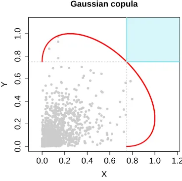
2.3.4 Scaled samples (grey) from a Gaussian copula with ρ = 0.5; the

cor-responding set G = {(x, y) ∈ _R2 _{: g(x, y) = 1} (red); and the set} [η{1,2},∞)2 (blue). . . 28

2.5.1 An example of a regular vine in five dimensions. . . 35

2.5.2 Four dimensional vine copula models;D-vine (left) and C-vine (right). 36

3.1.1 The simplex S2. Coordinates are transformed to the equilateral simplex. 41 3.4.1 Mean Hellinger distance, 0.05 and 0.95 quantiles over 100 simulations.

Method 1: purple; Method 2: green; Goix et al.: grey. . . 60

3.4.2 Plots to show the number of times each sub-cone is assigned mass

greater than π = 0.01 (top) and π = 0.001 (bottom), for (α, ρ) =

(0.75,0.5). Darker lines correspond to higher detection rates over 100

simulations. True sub-cones with mass: solid lines; sub-cones without

mass; dashed lines. . . 61

3.4.3 Stability plot (left) for Method 2, with dashed lines showing a 95%

bootstrapped confidence interval for the number of sub-cones with

mass, and a plot of the Hellinger distance (right) for each value of

δ. The shaded regions correspond to the stable range of tuning

param-eter values. Data were simulated from the max-mixture distribution of

Section 3.4.2 with n= 10,000, α = 0.25 andρ= 0.25. . . 63

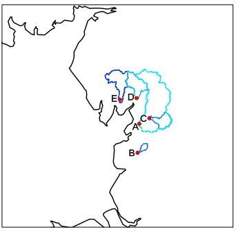
3.5.1 Locations of the river flow gauges (labelled A to E) and corresponding

catchment boundaries. . . 64

4.2.1 A partition of S2, with= 0.1; the coordinates are transformed to the equilateral simplex for visual purposes. . . 72

4.2.2 Comparison of regions B_C∗ (left) and BC (right) in Cartesian

coordi-nates; the paler blue regions are truncated to the axes. . . 73

4.2.3 An example of our proposed weighting in the trivariate case, with k=

10. The grey regions in the first two plots show where the weights are

exactly 0. . . 78

4.3.1 Mean Hellinger distance over 100 simulations for the max-mixture

dis-tribution. Method 1: purple; Method 2: green; Method 3: blue;

Method 4: pink; Method 5: orange; Goix et al.: grey. . . 80

4.3.2 Mean Hellinger distance over 100 simulations from asymmetric logistic

distributions withd= 5 (top row) andd= 10 (bottom row). Method 1:

purple; Method 2: green; Method 3: blue; Method 4: pink; Method 5:

4.3.3 Boxplots of AUC* values for Methods 3, 4 and 5 with d = 5; f =

5,10,15; n = 10,000 and α = 0.75. Mean AUC* values are shown by

the circles in each plot. . . 83

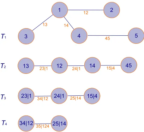
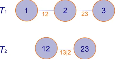
5.1.1 Graphical representation of a trivariate vine copula, with tree labels

T1,T2 as introduced in Section 2.5.3. . . 88 5.2.1 A scaled sample from a bivariate inverted logistic copula (left) and

bivariate logistic copula (right) with α = 0.5 (grey); the sets G =

{(x, y)∈_R2 _{:g(x, y) = 1} (red); and the sets [η}

{1,2},∞)2 (blue). . . . 91

5.3.1 Points in the set G = {x ∈ _R3 _{: g(x) = 1} for a trivariate vine} with three inverted logistic pair copula components (grey) and the set

[η{1,2,3},∞)3 (blue): α = 0.25 (left),α = 0.5 (centre), α= 0.75 (right); β = 0.25 and γ = 0.5. . . 97

5.3.2 Values of η{1,3} (dashed) and η{1,2,3} (solid) for a trivariate vine copula

with inverted logistic components, with α = 0.25 (left), α = 0.5

(cen-tre), α = 0.75 (right); β = 0.25 (red), β = 0.5 (purple) and β = 0.75

(orange); and γ ∈ (0.1,0.9). Average Hill estimates of η{1,3} (circles)

and η{1,2,3} (triangles) are provided in each case. . . 98

5.3.3 Left: g{1,3}(x1, x3) for (α, β, γ) = (0.5,0.25,0.5). Right: an approxima-tion of the corresponding sets G{1,3} (grey) and [η{1,3},∞)2 (blue). . 99

5.3.4 Graphical representations of four dimensional vine copula models; D

-vine (left) and C-vine (right). . . 101

5.3.5 Trivariate subsets of the four-dimensional D-vine. . . 103

5.3.6 Trivariate subsets of the four-dimensional C-vine. . . 106

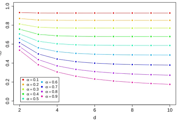
5.3.7 Values of ηD for d ∈ {2, . . . , d} for a d-dimensional D-vine or C-vine

with inverted logistic pair copulas with dependence parameters α ∈

5.4.1 Points in the set G = {x ∈ _R3 _{: g(x) = 1} for a trivariate vine with} inverted logistic copulas in T1 and a logistic copula in T2 (grey) and the set [η{1,2,3},∞)3 (blue): α= 0.25 (left), α= 0.5 (centre),α = 0.75

(right); β = 0.25 and γ = 0.5. . . 117

5.4.2 Left: g{1,3}(x1, x3) with (α, β, γ) = (0.5,0.25,0.5). Right: an approxi-mation of the corresponding sets G{1,3} (grey) and [η{1,3},∞)2 (blue). 118

5.5.1 Possible extremal dependence structures for trivariate vine copulas

con-structed from logistic and inverted logistic components. . . 122

6.3.1 MCMC chains for the scale and shape parameters for station 10 in June.131

6.3.2 Location of stations 2 (purple), 5 (pink), 7 (orange) and 10 (blue), as

well as estimates of the corresponding scale and shape parameters and

predicted 0.998 quantiles. . . 132

7.2.1 Average Hellinger distance, 0.05 and 0.95 quantiles over 25 simulations.

Method 1: purple; penalized censored log-likelihood: green. . . 137

7.2.2 Comparison of estimated τC values for cases (a)-(d) with α = 0.2 and

α = 0.8, over 25 simulations. The points show the average estimatedτC

value in each case. Method 1: purple; penalized censored log-likelihood:

green. . . 139

7.2.3 A sample of bivariate data exhibiting a mixture of asymptotic

depen-dence and asymptotic independepen-dence, and results from applying

Hamil-tonian Monte Carlo with 5000 iterations. True parameter values:

or-ange; mean of the posterior: solid pink; 90% credible interval; dashed

pink. . . 144

7.2.4 Extrapolation using the original approach of Heffernan and Tawn (top)

and our proposed two component mixture model (bottom); the orange

and blue regions show the two clusters. The original data are shown in

A.3.1Estimates of τ1(δ), τ1,2(δ) and τ1,2,3 for data simulated from trivariate logistic distributions with α= 0.25 (top) and α= 0.5 (bottom). . . . 159

A.3.2Area under the receiver operating characteristic curve results for 100

simulations from a five-dimensional max-mixture distribution. . . 160

A.3.3Area under the neighboured receiver operating characteristic curve

re-sults for 100 simulations from a five-dimensional max-mixture

distri-bution. . . 160

A.3.4Areas under the receiver operating characteristic curves for 100

simu-lations from a five-dimensional asymmetric logistic distribution. . . . 163

A.3.5Areas under the receiver operating characteristic curves for 100

simu-lations from a ten-dimensional asymmetric logistic distribution. . . . 163

A.3.6Boxplots of the areas under the neighboured receiver operating

charac-teristic curves for d = 5; f = 5,10,15; n = 10,000 and α = 0.75. The

average values are shown by the circles in each plot. . . 164

A.3.7Mean Hellinger distance, 0.05 and 0.95 quantiles over 100 simulations.

Method 1: purple; Method 2: green; Goix et al.: grey. . . 165

B.2.1AUC values for Methods 3, 4 and 5 over 100 simulations from a

five-dimensional max-mixture distribution. . . 170

B.2.2AUC* values for Methods 3, 4 and 5 over 100 simulations from a

five-dimensional max-mixture distribution. . . 171

B.3.1AUC results for Methods 3, 4 and 5 over 100 simulations from a

five-dimensional asymmetric logistic distribution. . . 171

B.3.2AUC results for Methods 3, 4 and 5 over 100 simulations from a

ten-dimensional asymmetric logistic distribution. . . 172

C.1.1Example of the extending a four-dimensionalD-vine to a five-dimensional

3.2.1 Values of τC(δ) for some trivariate copula examples. For all logistic

models the dependence parameter α satisfies 0< α <1, with larger α

values corresponding to weaker dependence. . . 49

3.4.1 Average area under the receiver operating characteristic curves, given

as percentages, for 100 samples from a five-dimensional mixture of

bi-variate Gaussian and extreme value logistic distributions; the standard

deviation of each result is given in brackets. . . 60

3.4.2 Average area under the neighboured receiver operating characteristic

curves, given as percentages, for 100 samples from a five-dimensional

mixture of bivariate Gaussian and extreme value logistic distributions;

the standard deviation of each result is given in brackets. . . 61

3.5.1 The percentage of mass assigned to each sub-cone for varying values of

the tuning parameters in Method 1 (left) and Method 2 (right). The

grey regions demonstrate the feasible stable ranges. . . 66

3.5.2 Estimated percentage of extremal mass on to each sub-cone when

con-sidering locations A-D, for varying values of the tuning parameters in

Method 1 (left) and Method 2 (right). . . 67

4.3.1 Average AUC (top) and AUC* (bottom) values, given as percentages,

for 100 samples from a five-dimensional max-mixture model. Results

in bold show where the methods are at least as successful as any of

those studied in Chapter 3. . . 81

4.3.2 Average AUC values, given as percentages, for Methods 3 and 4 over

100 samples from five-dimensional (top) and ten-dimensional (bottom)

asymmetric logistic distributions, with dependence parameter α.

Re-sults in bold show where the methods are at least as successful as any

of those studied in Chapter 3. . . 84

6.3.1 Percentage improvement over the benchmark for Challenges 1 and 2

across each month. . . 133

A.3.1Average areas under the receiver operating characteristic curves, given

as percentages, for 100 samples from five-dimensional (top) and

ten-dimensional (bottom) asymmetric logistic distributions, with

depen-dence parameter α and θi,C determined via (A.3.3). Standard

Introduction

1.1

Motivation

There are many situations where it may be necessary to understand and model

ex-treme values. Areas of interest range from environmental applications, such as high

river flows or extreme weather events, to financial ones, like stock market movements.

The occurrence of extreme events can have a huge impact, and a better understanding

of the types of extremes we may expect can help us to mitigate their effect.

One of the main issues faced in modelling extreme values is the often limited data

available; the events of interest may have never been observed, so standard statistical

modelling techniques may not apply. We therefore require a range of

asymptotically-motivated tools, which come from extreme value theory. A wide range of results are

available for modelling extremes, including classical approaches for univariate and

multivariate cases, as well as a variety of more recent advancements. There is

increas-ing interest in more complicated situations involvincreas-ing multivariate extremes, and there

is still work to be done to develop the theory and methodology necessary for these

circumstances; we focus on two such cases in this thesis.

Many existing methods for modelling multivariate extremes are only applicable

either if all of the variables take their largest values simultaneously, or if they occur

separately in each one. However, in some scenarios it is possible for certain subsets

of the variables to take their largest values simultaneously while the others are small,

and models for the extreme values should reflect this. We aim to develop methods to

determine these possibly complex extremal dependence structures, with the ultimate

aim being to aid model selection.

We also consider the case where there is a specific underlying dependence structure

among the variables. The example we focus on is vine copulas (Joe, 1996; Bedford and

Cooke, 2001, 2002), which are a class of multivariate model constructed from a series

of bivariate copulas, and whose dependence structure can be represented graphically.

Owing to their flexibility, vine copulas have grown in popularity in recent years, and

have the potential to be used for modelling multivariate extremes. We investigate

how imposing the graphical dependence structure of vine copulas influences the tail

dependence properties that can be captured by such models.

1.2

Outline of thesis

The overall aim of this thesis is to develop methods for assessing and modelling

de-pendence in multivariate extremes. There already exists a rich literature in this area;

we aim to build on this work with some novel approaches, which are outlined in this

section.

Chapter 2 gives an overview of some of the techniques that can be used in extreme

value modelling. We begin with a brief introduction to some of the standard methods

for modelling univariate extremes, before reviewing existing methods for multivariate

In Chapter 3, we introduce methodology for determining the dependence structure

of multivariate extremes; that is, the subsets of variables that can take their largest

values simultaneously, while the others are of smaller order. Under a regular

varia-tion assumpvaria-tion, we present a new set of indices that reveal aspects of the extremal

dependence structure not available through any existing measures of dependence. We

derive theoretical properties of these indices, demonstrate their value through a

se-ries of examples, and develop inferential methods that also allow us to estimate the

proportion of extremal mass associated with each subset of variables. We apply the

methods to UK river flows, estimating the probabilities of different subsets of sites

being large simultaneously.

In Chapter 4, we present alternative methods for determining extremal

depen-dence structures; this time in a radial-angular setting. The first of these is a

simplex-partitioning approach based on a regular variation assumption. This setting also

enables us to introduce a soft-thresholding approach that allows the information from

each observation to be shared across multiple faces. This is achieved by assigning

weights to points in the angular simplex based on their proximity to the various faces.

We also implement this soft-thresholding technique to extend the approach of Goix

et al. (2016). We compare the simplex-partitioning method and both these weighted

approaches to the methods in Chapter 3 via a simulation study, using receiver

op-erating characteristic curves to test their performance as classifiers, and comparing

Hellinger distances to assess the estimation of the proportion of extremal mass

as-signed to each face of the angular simplex. In several cases in this simulation study,

these radial-angular methods show improvement over those in Chapter 3.

In Chapter 5, we investigate some of the tail dependence properties of vine

certain sub-classes of this model. We focus on the trivariate case, and vine copulas

constructed from extreme value and inverted extreme value pair copulas. We follow

the approach of Nolde (2014), who investigates the limiting shape of suitably-scaled

sample clouds to give a geometric interpretation of η, which allows for calculation

of this coefficient from a joint density. By extending this theory, we propose a way

to calculate η for multivariate margins when the joint density can only be expressed

analytically for a higher order multivariate distribution. We also consider using

nu-merical approximation for cases where η cannot be found analytically.

Chapter 6 was written following entry of a STOR-i team to the EVA2017

chal-lenge. The aim of the challenge was to predict extreme precipitation quantiles across

several sites in the Netherlands. Our proposed method uses a Bayesian hierarchical

structure, and a combination of Gamma and generalized Pareto distributions. We

impose a spatio-temporal structure in the model parameters via an autoregressive

prior, and propose estimating model parameters using Markov chain Monte Carlo

techniques and spatial interpolation. Our approach was successful in the context

of the challenge, providing reasonable improvements over the benchmark method in

terms of the quantile loss function of Koenker (2005).

In Chapter 7, we summarize the contributions of this thesis, and discuss some

possible avenues for future work. The latter includes an alternative parameter

esti-mation method for the approaches of Chapter 3, and a way to deal with negligible

mass assigned to faces of the angular simplex in the methods of Chapters 3 and 4.

We also propose a mixture model based on the conditional extreme value modelling

approach of Heffernan and Tawn (2004) that has the potential to capture different

combinations of tail dependence features; we suggest using Hamiltonian Monte Carlo

Literature Review

2.1

Introduction

When studying extreme events, we are concerned with the tails of a distribution, where

the intrinsically small number of observations make statistical modelling a challenge.

We may also be interested modelling events that have not been observed in the data,

meaning that extrapolation is a key concern. Due to the usually limited amount of

data, empirical methods and other standard statistical techniques may not be

appli-cable; we instead require results from extreme value theory.

In this chapter, we introduce some of the methods currently available to model

extreme events. We begin with an overview of classical results for modelling

univari-ate extremes in Section 2.2, before discussing multivariunivari-ate techniques in Section 2.3.

In Section 2.4, we discuss existing ideas for modelling multivariate extremes where

there is some underlying structure controlling the dependence between the variables.

Finally, we introduce a class of multivariate models known as vine copulas in

Sec-tion 2.5; these models also have a specific dependence structure which can be

repre-sented graphically, and could be exploited in multivariate extreme value modelling.

2.2

Univariate extreme value theory

2.2.1

Overview

A thorough review of standard methods for modelling univariate extremes can be

found in Coles (2001). Here, we discuss some of the main results, including two

common approaches for modelling univariate extremes, based on the generalized

extreme value (GEV) and generalized Pareto (GP) distributions, discussed in

Sec-tions 2.2.2 and 2.2.3, respectively.

2.2.2

Generalized extreme value distribution

LetX1, . . . , Xn be independent random variables with common distribution function

F. The upper tail of distribution F can be modelled by considering

Mn = max(X1, . . . , Xn).

By the extremal types theorem of Leadbetter et al. (1983), if there exist seriesan>0

and bn such that

Pr

Mn−bn

an

≤x

→G(x),

as n → ∞, with G non-degenerate, then G belongs to the family of extreme value

distributions, and the distribution functionF of each of theXi variables is said to lie

in the domain of attraction of G.

The distribution function G corresponds to either a negative Weibull, Fr´echet or

Gumbel distribution, and these three cases can be combined into a single family of

the form

G(x) = exp

(

−

1 +ξ

x−µ σ

−1/ξ

+

)

, (2.2.1)

with location parameter µ ∈ (−∞,∞), scale parameter σ ∈ (0,∞) and shape

generalized extreme value (GEV) distribution. For ξ < 0, this corresponds to the

negative Weibull distribution; for ξ > 0, the distribution is Fr´echet; and the GEV

distribution withξ= 0 (interpreted asξ →0) corresponds to a Gumbel distribution.

Assuming that equation (2.2.1) holds exactly for large n, we have

Pr(Mn ≤x) =G

x−bn

an

= ˜G(x),

where ˜G represents a GEV distribution with different location and scale parameters

toG. This result allows us to use the GEV distribution to model maxima in practice.

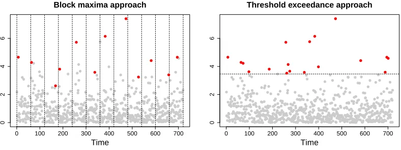
A common method in modelling univariate extremes is to use the block maxima

approach, where data are separated into sections of equal length, and the maximum

value observed in each block is considered to be a realization of a GEV random

variable; this is demonstrated in the left panel of Figure 2.2.1. The maximum observed

values from the different blocks are used for inference of the GEV parameters.

0 100 200 300 400 500 600 700

0

2

4

6

Block maxima approach

Time

0 100 200 300 400 500 600 700

0

2

4

6

Threshold exceedance approach

Time

Figure 2.2.1: A demonstration of the data considered extreme in the block maxima

and threshold exceedance methods.

Theory for modelling the lower tail of a distribution can be derived from the theory

for the upper tail by exploiting the relation

min(X1, . . . , Xn) =−max(−X1,· · · −Xn).

2.2.3

Generalized Pareto distribution

A common criticism of the block maxima approach is that taking only one value per

block may lead to some information about extreme events being disregarded. A

typi-cal alternative is to consider values above a high threshold,u, as being extreme, and

to fit a model to the exceedances above that threshold. This method generally

uti-lizes more of the extreme observations than the block maxima approach; an example

is shown in the right panel of Figure 2.2.1.

A model for threshold exceedances can be motivated via the point process

represen-tation of Pickands (1971). Suppose we have independent and identically distributed

random variablesX1, . . . , Xn, whose common distribution function F has upper

end-point xF, and that there exist an > 0 and bn such that Pr{(Mn−bn)/an≤x} →

G(x), where G follows a GEV distribution. As n → ∞, it can be shown that the

point process

Pn =

i n+ 1,

Xi−bn

an

:i= 1, . . . , n

converges to a non-homogeneous Poisson process,P, with integrated intensity

Λ [c1, c2]×[x,∞)

= (c2−c1)

1 +ξ

x−µ σ

−1/ξ

+

, (2.2.2)

on [0,1]×[xG,∞), for xG = inf{x : G(x) > 0} and 0 < c1 < c2 < 1. Coles (2001), for example, demonstrates that a model for threshold exceedances may be obtained

from this limiting Poisson process result. First note that the integrated intensity in

(2.2.2) may be written as

Λ [c1, c2]×(x,∞)

= Λ1 [c1, c2]

×Λ2 [x,∞)

,

with

Λ1 [c1, c2]

=c2−c1 and Λ2 [x,∞)

=

1 +ξ

x−µ σ

−1/ξ

+

.

Then, foru > xG, we have

Pr

Xi−bn

an

≤x+u

Xi−bn

an

> u

= 1−Pr

Xi−bn

an

> x+u

Xi−bn

an

> u

→1− Λ2 [x+u,∞)

Λ2 [u,∞) , as n→ ∞ = 1−

1 +ξ x+u_σ−µ−1/ξ

+

1 +ξ u−_σµ−₊1/ξ

= 1−

1 + ξx

σu

−1/ξ

+

=:H(x), (2.2.3)

where σu = σ +ξ(u−µ). Distributions of the form H(x) are termed generalized

Pareto (GP) distributions.

By a similar argument as for the GEV distribution, treating (2.2.3) as an equality

for largen, we may disregard the constants an and bn for modelling purposes. To see

this, first note that by (2.2.3), for large u, we have

Pr (Xi > anx+anu+bn |Xi > anu+bn) =

1 + ξx

σu

−1/ξ

+

.

Now, settingun =anu+bn, and y=anx,

Pr (Xi > y+un |Xi > un) =

1 + ξx

σu,n

−1/ξ

+

,

which corresponds to a generalized Pareto distribution with scale parameter σu,n =

anσu. As the threshold un tends towards xF, exceedances above un may therefore be

modelled using the GP distribution.

We can fit both GEV and GP distributions numerically using standard maximum

likelihood techniques. One of the main issues that arises when carrying out inference

for the GP distribution is choosing a suitable value for the threshold. This must be

small enough that we have sufficient data to fit the model, but large enough that the

results provide a valid asymptotic approximation. One simple approach is to consider

parameter stability plots, as outlined by Coles (2001), in which parameter estimates

are observed over a range of threshold choices. An issue here is that stability plots

meaning they are often difficult to interpret. To overcome this, Wadsworth (2016)

proposes an alternative threshold selection method based on the joint distribution

of the estimated model parameters, and discusses a way to automate this method,

avoiding the need to interpret plots by eye. There is a large amount of further research

on the topic of threshold selection; a review of many of these techniques is given by

Scarrott and MacDonald (2012), while more recent approaches include a Bayesian

cross-validation technique proposed by Northrop et al. (2017).

2.3

Multivariate extreme value theory

2.3.1

Defining extreme events

Unlike in the univariate case where we consider maxima and minima, there is no

clear, single way to define an extreme event for multiple variables. The most suitable

definition of an extreme event will usually depend on context; Barnett (1976) suggests

several possibilities. One of the most common ways of defining a multivariate extreme

event is to consider componentwise maxima, i.e., the maximum of each variable, which

may not correspond to an actual observation. Alternatives include defining a convex

hull around the data, with points lying on or beyond this region deemed extreme;

considering observations which contain the maximum of at least one variable; and

defining some function of the data, which may allow transformation of the problem

to the univariate setting, as considered by Coles and Tawn (1994).

2.3.2

Copula theory

In multivariate modelling, it is important to consider the dependence properties of

the variables. Copulas provide a way to separate marginal modelling from

depen-dence modelling, which is often useful in practice. Joe (1997) and Nelsen (2006) give

recent developments in the area.

By Sklar’s theorem (Sklar, 1959), ifX = (X1, . . . , Xd) has joint distribution

func-tion F, and Xi ∼ Fi, for i = 1, . . . , d and each Fi continuous, then there exists a

unique copulaC such that

F(x1, . . . , xd) = C{F1(x1), . . . , Fd(xd)}.

The copula C is essentially a distribution function with Uniform(0,1) marginal

dis-tributions, and determines the dependence structure of the variables. This result,

alongside the probability integral transform, allows for transformation between

differ-ent marginal distributions while preserving the dependence properties of the variables.

If Xi is a continuous random variable with distribution function Fi and inverse

distribution function F_i−1, then by the probability integral transform, U = Fi(X) ∼

Uniform(0,1), and F_i−1(U) ∼ Fi. So for instance, we may obtain a copula CF with

standard Fr´echet margins via

F(x1, . . . , xd) =CF

− 1

logF1(x1)

, . . . ,− 1

logFd(xd)

,

a copula CE with standard exponential margins is defined by

F(x1, . . . , xd) = CE[−log{1−F1(x1)}, . . . ,−log{1−Fd(xd)}],

and for standard Gumbel margins, the copulaCG satisfies

F(x1, . . . , xd) = CG[−log{−logF1(x1)}, . . . ,−log{−logFd(xd)}].

Analogous results can be used for transformation to other marginal distributions.

These results are often used in multivariate extreme value theory, where

transform-ing margins can highlight particular features of the extreme values. In the Fr´echet

0.0 0.2 0.4 0.6 0.8 1.0

0.0

0.2

0.4

0.6

0.8

1.0

Uniform

XU YU

0 1000 3000 5000 7000

0

1000

3000

5000

7000

Frechet

XF YF

0 2 4 6 8

0

2

4

6

8

Exponential

XE YE

−2 0 2 4 6 8

−2

0

2

4

6

8

Gumbel

XG YG

Figure 2.3.1: Example of data transformed to different marginal distributions.

are used in the conditional approach of Heffernan and Tawn (2004), discussed in

Sec-tion 2.3.11, to focus on the behaviour of variables given that one of the variables is

extreme. A demonstration of data transformed to different marginal distributions is

given in Figure 2.3.1, for data simulated from a bivariate extreme value logistic

dis-tribution with dependence parameter α= 0.75. This model will be discussed further

in Section 2.3.3.

2.3.3

Componentwise maxima

Consider n independent d-dimensional random vectors X1, . . . , Xn with common

distribution function F. We denote the vector of componentwise maxima by Mn =

(Mn,1, . . . , Mn,d), where Mn,i = maxj∈{1,...,n}Xj,i, for i = 1, . . . , d, and Xj,i denotes

element i of the vector Xj. In a similar way to the univariate case, suppose there

exist constants an,i>0 and bn,i, fori= 1, . . . , d, such that

Pr

Mn,1−bn,1

an,1

≤x1, . . . ,

Mn,d−bn,d

an,d

≤xd

→G(x1, . . . , xd),

as n → ∞, for some limiting distribution function G that is non-degenerate in each

margin. Unlike in the univariate case, the distributionG does not have a single

para-metric form, although each of the marginal distributions of Gis a GEV distribution.

Setting identical margins is often the easiest way in practice to study the properties of

by the copula theory in Section 2.3.2. Choosing standard Fr´echet marginal

distribu-tions emphasizes the largest values, as demonstrated in Figure 2.3.1; this is therefore

the usual choice for modelling componentwise maxima. In particular, ifXi has a unit

Fr´echet distribution for each i= 1, . . . , d, so that Pr(Xi < x) = exp(−1/x) for x >0,

Gmay be written as

G(x) = exp{−V(x)}, (2.3.1)

where x = (x1, . . . , xd) andxi > 0 for i = 1, . . . , d. The function V is known as the

exponent measure, and, forSd−1 =

w∈[0,1]d _:Pd

i=1wi = 1 , takes the form

V(x) = d

Z

Sd−1

max

i=1,...,d

wi

xi

dH(w), (2.3.2)

whereH is termed the spectral measure and, for i= 1, . . . , d, satisfies

Z

Sd−1

widH(w) =

1

d. (2.3.3)

Special cases include independence between X1 and X2, where V (x1, x2) = x−11 +

x−₂1 and H({0}) = H({1}) = 1/2; and perfect dependence, which corresponds to

V (x1, x2) = max x−11, x

−1 2

and H({1/2}) = 1.

Functions G(x) satisfying (2.3.1) are termed multivariate extreme value

distribu-tions. Several parametric models of this form have been proposed in the literature,

including the logistic distribution of Gumbel (1960), for which the exponent measure

is

V(x) =

d

X

i=1

x−_i1/α

!α

, (2.3.4)

for α ∈ (0,1]. For this model, taking α = 1 leads to independence between the

variables, while as α → 0 we approach the case of complete dependence; in general,

smaller values ofαcorrespond to stronger dependence between the variables. Another

case by Tawn (1988), and extended to the multivariate setting by Tawn (1990). The

exponent measure for the asymmetric logistic distribution has the form

V(x) = X

C∈2D_\∅

( X

i∈C

θi,C

xi

1/αC)αC

, (2.3.5)

withαC ∈(0,1],θi,C ∈[0,1],θi,C = 0 if i /∈C, and

P

C∈2D_\∅

θi,C = 1 for all i= 1, . . . , d,

andC ∈2D\∅, where 2D denotes the power set ofD={1, . . . , d}. The parametersαC

control dependence in a similar way toαin the logistic model, although this time just

for the corresponding subsets of the variables. Other parametric models belonging

to the class of multivariate extreme value distributions include the negative logistic

model of Galambos (1975); the negative asymmetric logistic model of Joe (1990); and

the H¨usler-Reiss distributions (H¨usler and Reiss, 1989).

Ledford and Tawn (1997) propose inverting models of the form (2.3.1) for the

case where d = 2, so that the joint lower tail becomes the joint upper tail, and vice

versa. The resulting class of models are known as inverted bivariate extreme values

distributions, with copula of the form

C(u, v) = u+v −1 + exp

−V

−1

log(1−u),

−1

log(1−v)

. (2.3.6)

These models exhibit different tail dependence properties to the corresponding

ex-treme value distributions, and will be discussed further in Sections 2.3.7 and 2.3.10.

2.3.4

The linking between

V

and

H

The exponent measure V and spectral measure H are related, due to the definition

of V in (2.3.2), and Coles and Tawn (1991) show that these measures are linked via

further relations. Specifically, in the bivariate case, they show that

h(w) = −(x1 +x2)

3 2

∂2 ∂x1∂x2

V(x1, x2), for w∈(0,1),

H({0}) = −x

2 2 2

∂ ∂x2

V(x1, x2)

and H({1}) = −x 2 1 2 ∂ ∂x1

V(x1, x2)

x2=0 .

A similar result for thed-dimensional case links the exponent measureV and spectral

densityh via

h x

Pd i=1xi

!

=−

Pd

i=1xi

d+1

d

∂d

∂x1, . . . , ∂xd

V(x).

Moreover, for any subset of variables XC = {Xi : i ∈ C} for C ∈ 2D \ ∅ and

D={1, . . . , d}, Coles and Tawn (1991) show that the spectral density hC for events

that are extreme only in XC is given by

hC

 

xC

P

i∈C

xi

 =−

P

i∈C

xi

|C|+1

|C|

Y

i∈C

∂ ∂xi

!

V(x). (2.3.7)

For instance, consider the asymmetric logistic model with exponent measure (2.3.5).

In this case, applying (2.3.7), we find that the spectral density corresponding to the

setC is given by

hC(wC) =−

P

i∈C

xi

|C|+1

|C|

  

|C|−1

Y

i=0

i−αC

αC    Y

i∈C

θ1/αC

i,C

x1+1/αC

i

! ( X

i∈C

θi,C

xi

1/αC)αC−|C|

,

forwC =xC/

P

i∈C

xi.

2.3.5

Pickands’ dependence function

In the bivariate case, again with standard Fr´echet margins, the exponent measure

V(x1, x2) links to Pickands’ dependence functionA(w) (Pickands, 1981) via the equa-tion

V(x1, x2) =

1 x1 + 1 x2

A(w),

for w=x1/(x1+x2), i.e., 0 ≤w ≤1. Pickands’ dependence function is convex, and has the conditions that A(0) = A(1) = 1, and max(w,1− w) ≤ A(w) ≤ 1. The

dependence,A(w) = max(w,1−w). These cases highlight a drawback of the

compo-nentwise maxima approach for modelling the joint upper tail of (X1, X2); sinceA(w) is a convex function, with independence and perfect dependence as boundary cases,

it is not possible to model negative dependence using these componentwise maxima

results.

Pickands’ dependence function also links to the spectral measureHby the relations

dA

dw = 2H(w)−1 and d2_A

dw2 = 2

dH

dw = 2h(w),

whereh(w) is the density corresponding to the spectral measure H.

2.3.6

Regular variation

An alternative tail characterization of X is in terms of its pseudo-polar coordinates (R,W). Consider the random vector X = (X1, . . . , Xd), with common marginal

distributions satisfying Pr(Xi > x) ∼ cx−1 for i = 1, . . . , d and some c > 0. For

arbitrary norms, k · k1 and k · k2, the coordinates (R,W) are defined as

R =kXk1 and W =X/kXk2,

with R > 0 and W ∈ Sd−1 =

(w1, . . . , wd) ∈ [0,1]d : Pd_i=1wi = 1 , the (d−

1)-dimensional unit simplex.

Taking both norms to be the L1 norm, i.e., kxk1 =kxk2 =Pd_i=1xi, the

assump-tion of multivariate regular variaassump-tion states that

lim

t→∞Pr(R > tr,W ∈B |R > t) =H(B)r

−1_{, (2.3.8)}

forr≥1, spectral measureHsatisfying (2.3.3) andB some measurable subset ofSd−1. The right-hand side of (2.3.8) shows that under the regular variation assumption, we

values, the position of angular mass onSd−1links to the extremal dependence structure of X, i.e., the subsets of X that can take their largest values simultaneously, which will be discussed further in Section 2.3.8.

2.3.7

Modelling asymptotic dependence

Many methods for modelling multivariate extremes are only applicable for variables

with certain tail dependence properties, and an important consideration is whether

or not the variables can take their largest values simultaneously. It is useful for model

selection to have measures that allow us to categorize data as belonging to different

tail dependence classes. Several such methods are discussed by Coles et al. (1999);

we focus on one such measure here, denoted by χ.

In the bivariate case, consider variables X1 and X2 with respective distribution functionsF1 andF2. The measureχ, taking values in [0,1], is defined via the limiting conditional survivor function

χ= lim

u→1Pr{F2(X2)> u|F1(X1)> u}= limu→1

Pr{F1(X1)> u, F2(X2)> u}

1−u ,

where the limit is assumed to exist. In this case, if χ = 0, the variables are said

to be asymptotically independent, i.e., X1 and X2 cannot take their largest values simultaneously, while ifχ ∈ (0,1], the variables may be simultaneously extreme and

are said to exhibit asymptotic dependence.

For a bivariate extreme value distribution with exponent measure V(x1, x2) and distribution function of the form (2.3.1), we have

χ= lim

u→1Pr{F2(X2)> u|F1(X1)> u} = lim

u→1

1−2u+ exp{−V(−1/logu,−1/logu)}

1−u = limu→1

1−2u+uV(1,1) 1−u

= lim

u→1

1−2u+ 1 +V(1,1)(u−1) +O{(u−1)2_}

This implies that the bivariate logistic model with exponent measure (2.3.4) hasχ=

2−2α_{. That is, it exhibits asymptotic dependence for α ∈ (0,1), and asymptotic}

independence forα= 1, which corresponds to the independence case. The asymmetric

logistic model with exponent measure (2.3.5) has

χ=θ1,{1,2}+θ2,{1,2}−

θ1/α{1,2}

1,{1,2} +θ

1/α{1,2}

2,{1,2}

α{1,2}

.

For this model, if α{1,2} = 1, or if θ1,{1,2} = θ2,{1,2} = 0, we are in the independence

setting withχ= 0. Otherwise, the model exhibits asymptotic dependence. Examples

of models withχ= 0, corresponding to asymptotic independence, include the

bivari-ate Gaussian and inverted bivaribivari-ate extreme value distributions in (2.3.6).

The idea of using a limiting conditional probability to assess tail dependence

ex-tends naturally to a multivariate setting. Suppose we are interested in the random

vector X = (X1, . . . , Xd) with Xi ∼ Fi for each i ∈ D = {1, . . . , d}. To investigate

the tail dependence properties of a subset of variables XC = {Xi : i ∈ C} for some

C∈2D _{with |C| ≥2, a suitable measure of tail dependence is}

χC = lim u→1

Pr{Fi(Xi)> u:i∈C}

1−u , (2.3.9)

see for example Hua and Joe (2011) or Wadsworth and Tawn (2013). In this case, if

χC ∈(0,1], the variables XC are asymptotically dependent, i.e., all components can

be large simultaneously. On the other hand, if χC = 0, the variables in XC cannot

all take their largest values together, although any subsetC ⊂C with |C| ≥2 could

haveχC >0, that is, XC could still exhibit asymptotic dependence.

As an example, consider the asymmetric logistic model with only pairwise

depen-dence, i.e., with exponent measure

V(x1, x2, x3) =

(

θ1

x1

1/α1

+

θ2

x2

1/α1)α1

+

(

1−θ1

x1

1/α2

+

θ3

x3

1/α2)α2

+

(

1−θ2

x2

1/α3

+

1−θ3

x3

with α1, α2, α3 ∈ (0,1] and θ1, θ2, θ3 ∈ [0,1], where the parameter subscripts have been simplified from (2.3.5) to improve readability. In this case, it can be shown that

χ{1,2,3} = 0, while the bivariate measures of dependence are

χ{1,2} =θ1+θ2−

θ1/α1

1 +θ 1/α1

2

α1

, χ{1,3} = 1−θ1+θ3−

n

(1−θ1)1/α2 +θ 1/α2

3

oα2 ,

and χ{2,3} = 1−θ2 + 1−θ3−

(1−θ2)1/α3 _{+ (1−θ3)}1/α3 α3_.

That is, this particular model does not exhibit overall asymptotic dependence, but

can still have asymptotic dependence in all pairs of variables if α1, α2, α3 6= 1 and

θ1, θ2, θ3 ∈(0,1).

2.3.8

Extremal dependence structures

The definition ofχC in the previous section demonstrates that extremal dependence

in multivariate extremes can have a complicated structure, with only certain subsets

of the variables being simultaneously large while other variables are of smaller order.

In the radial-angular representation of Section 2.3.6, this corresponds to the spectral

measureH placing extremal mass on various faces of the angular simplex Sd−1. The

extremal dependence properties exhibited by a particular set of data should be

con-sidered when selecting a model for its extreme values; we should aim to match the

extremal dependence structure of the data to the structures that proposed models

can capture. Many parametric models for multivariate extremes are only suitable

for the asymptotic dependence or asymptotic independence cases, such as the logistic

model with α ∈ (0,1) and the multivariate Gaussian, respectively. However, some

models, such as the asymmetric logistic model with exponent measure (2.3.5) allow

for more complicated extremal dependence structures. In particular, ifP

i∈Cθi,C >0

forC ∈2D\ ∅, the asymmetric logistic distribution places extremal mass on the face of Sd−1 corresponding to the variables {Xi :i ∈C} being simultaneously large while

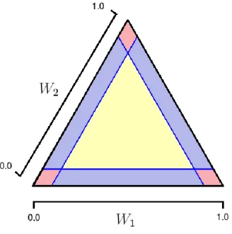
Figure 2.3.2: Example of a trivariate distribution with mass on five faces of the angular

simplex. The data are generated using a multivariate extreme value distribution with

an asymmetric logistic model.

Figure 2.3.2 shows an example of data simulated from the asymmetric logistic

distribution with the dependence parameters αC = 0.6 for allC ∈2D \ ∅, controlling

how close to the centre of the faces with mass the extremal points lie. The

depen-dence structure has been chosen to correspond to limiting mass on two of the vertices,

two of the edges and the centre of the unit simplex. In particular, X1 and X3 can both take their largest values independently of the other variables, and the subsets

{X1, X2}, {X2, X3} and {X1, X2, X3} may be simultaneously large. Here, we have

taken a sample of size n = 10,000, and the three plots show (W1, W2) |R > r, with

r taken to be the observed 0.9, 0.95 and 0.99 radial quantiles, respectively. The data

in Figure 2.3.2 are presented on the equilateral simplex for visual purposes.

As we increase the radial threshold, we observe that, although there are points

close to the boundaries of the unit simplex, none of these points lie exactly on the

boundary, so simply considering the proportion of points on each face above a high

threshold does not reveal the extremal dependence structure. Moreover, there

ap-pears to be mass close to all three corners of the unit simplex, when in fact only two

de-pendence structure of the variables using such data, conditioning onR being above a

finite threshold, we need to determine which faces truly represent this limiting

depen-dence structure, and which faces appearing to have mass do so as an artefact of lack

of convergence at finite levels. We propose methods for determining this structure

in Chapters 3 and 4, and introduce some existing methods in the remainder of this

section.

Goix et al. (2016) propose a non-parametric simplex-partitioning method for

es-timating extremal dependence structures. In this approach, the different regions of

the partition are chosen to estimate the various faces of the angular simplex Sd−1, with extremal mass on each of these faces corresponding to a different subset of the

variables being simultaneously extreme while the others are of smaller order.

Condi-tioning on the radial component being above some high threshold, empirical estimates

are obtained for the amount of extremal mass associated with each face, and a sparse

representation of the extremal dependence structure is obtained by considering faces

where this empirical estimate is sufficiently large. This method is shown to work well

in practice, particularly when the asymptotic dependence between variables in the

same subsets is strong.

In the method proposed by Goix et al. (2016), the aim is to obtain a

representa-tion of the extremal dependence structure that is sparse, i.e., the number of subsets

of variables being simultaneously large should be small compared to the dimension of

the problem. Chiapino and Sabourin (2017) point out that sparsity may not always

be achieved by this method, as too many faces that are similar in some way could be

detected. They therefore propose an algorithm that aims to group together nearby

faces with extremal mass into feature clusters. This method exploits the graphical

structure of clusters, and uses a measure of extremal dependence related toχto group

(2019) extend this approach by using the coefficient of tail dependence of Ledford and

Tawn (1996), discussed in Section 2.3.9, to assess the extremal dependence of groups

of variables. Our approaches in Chapters 3 and 4 exploit a new set of parameters,

related to this coefficient of tail dependence, that reveal additional information about

the extremal dependence structure.

Extremal dependence structures have also been studied elsewhere in the literature.

This includes the factor analysis approach of Kl¨uppelberg et al. (2015) for elliptical

copulas; the method of Chautru (2015) which incorporates principal component

anal-ysis and clustering techniques; and the Bayesian clustering approach of Vettori et al.

(2018).

2.3.9

Modelling asymptotic independence

Our focus so far has mainly been on modelling asymptotic dependence between

vari-ables; we now consider asymptotic independence in more detail. The approach of

Ledford and Tawn (1996) allows for the modelling of both asymptotic independence

and asymptotic dependence, with the latter a boundary case. For random variables

X1 and X2 with common marginal distribution F with an infinite upper endpoint, they propose a model for the limiting behaviour of the joint survivor function. This

is given by

Pr(X1 > x, X2 > x)∼L

{1−F(x)}−1

{1−F(x)}1/η_{, (2.3.10)}

as x→ ∞, for η ∈(0,1] and some function L that is slowly varying at infinity, that

isL(tx)/L(t)→1 ast→ ∞ for allx >0. This is often presented for (X1, X2) having standard Fr´echet margins, so that asx→ ∞,

Pr(X1 > x, X2 > x)∼L(x)x−1/η.

If η = 1 and L(x) 6→ 0 as x → ∞, there is asymptotic dependence between the

used to determine the tail dependence properties of a given pair of variables. If we

haveη <1, the particular value of ηand the function Lare indicative of the strength

of asymptotic independence between the variables, with η = 1/2 corresponding to

exact independence ifL(x) = 1 or near independence for L(x)6= 1, and the variables

having some positive association forη ∈(1/2,1).

A similar approach can be adopted in the multivariate case, as considered, for

instance, by de Haan and Zhou (2011) and Eastoe and Tawn (2012). For the random

vectorX = (X1, . . . , Xd) with standard Fr´echet margins, and any setC∈2D\ ∅ with

D={1, . . . , d}, we can study

Pr(Xi > x:i∈C)∼LC(x)x−1/ηC,

as x→ ∞, for some slowly varying function LC, ηC ∈ (0,1]. In this case, if ηC = 1,

there is asymptotic dependence between the variables XC = {Xi : i ∈ C}. For

ηC <1,XC exhibits asymptotic independence, although it could still be the case that

certain subsets of the variables can be large together, relating to the more complicated

extremal dependence structures discussed in Section 2.3.8.

Inference for the parameter ηC is not straightforward since estimation of the

pa-rameter is difficult, and the value corresponding to asymptotic dependence is a

bound-ary case. One standard approach is to use the Hill estimator (Hill, 1975). Consider

ordered realizations t(1) > t(2) > · · · > t(n) of the variable T = min(Xi : i ∈ C).

Assuming model (2.3.10) holds exactly for x above some high threshold u, the Hill

estimate can be derived using maximum likelihood techniques as

ˆ

ηC =

1

nu nu

X

i=1 log

t(i)

u

, (2.3.11)

where nu denotes the number of realizations above the threshold u. In practice, this

can take values greater than 1, so we often take ˆηC to be the minimum of 1 and

via the Hill estimate. In particular, they comment that uncertainty in the

parame-ter estimation is often underestimated in practice, which could, for instance, lead to

likelihood ratio tests incorrectly rejecting asymptotic dependence. In our studies, we

found that the Hill estimate is often lower than the true value of ηC, particularly if

this true value is 1 or close to 1, also leading to difficulty in distinguishing between

asymptotic dependence and asymptotic independence. This is an issue we investigate

further in Section 7.2.2 in the context of the methods we propose in Chapters 3 and 4.

A review of other techniques for estimating ηC can be found in Section 9.5.2

of Beirlant et al. (2004). These include procedures developed by Peng (1999) and

Draisma et al. (2004), who suggest non-parametric estimates ofηC that do not depend

on the marginal distributions of the variables, and Beirlant and Vandewalle (2002)

whose approach is based on scaled log-ratios.

2.3.10

Calculating the coefficient of tail dependence from a

density

The coefficient of tail dependence ηC is defined in terms of the survivor function of

the variablesXC. However, for certain distributions, it may not be possible to obtain

this function analytically, and it may only be the joint density that is available. Nolde

(2014) presents a strategy for determining ηC in this setting using a geometric

ap-proach, by considering the shape of scaled random samples from the joint distribution

of XC.

Assuming standard exponential margins, and that the variables XC have joint

densityf(x), Nolde proposes studying the gauge functiong(x), which is homogeneous

of order 1, such that

as t → ∞. Interest then lies with the set G = {x ∈ _R|C| _{: g(x) = 1}, which}

forms the boundary of the scaled random sample (XC,1/logn, . . . ,XC,n/logn) for

largen, where the scaling function logn is chosen due to the exponential margins. In

particular, note that for each variable Xi, i∈C, with Mi,n= max(Xi,1, . . . , Xi,n),

Pr

Mi,n

logn < x

= 1−e−xlognn=

1− 1

nx

n

→

        

0, x <1,

e−1, x= 1,

1, x >1,

as n → ∞, so that, asymptotically, Mi,n/logn = 1. As such, the set G lies within

the region [0,1]|C|. The coefficient ηC corresponds to the smallest value of r such

that G∩[r,∞)|C| _{= ∅ (or the largest value of r such that G∩[r,∞)}|C| _{6= ∅). We}

demonstrate this approach using a series of bivariate examples.

Let us first consider an inverted bivariate extreme value distribution. In

exponen-tial margins, this model has distribution function

F(x, y) = 1−e−x−e−y+ exp−V x−1, y−1 ,

for x, y > 0. By first differentiating with respect to both components to obtain the

densityf(x, y), with V1, V2 and V12 denoting the derivatives of the exponent measure with respect to the first, second and both components, respectively, we have

−logf(tx, ty) =2 log(tx) + 2 log(ty) +V

(tx)−1,(ty)−1

−log

V1

(tx)−1,(ty)−1 V2

(tx)−1,(ty)−1 −V12

(tx)−1,(ty)−1

= 2 log(tx) + 2 log(ty) +tV x−1, y−1

−logt4V1 x−1, y−1

V2 x−1, y−1

−t3V12 x−1, y−1

=tV x−1, y−1+O(logt),

ast→ ∞, by exploiting the homogeneity of the exponent measure. That is, the gauge

For the bivariate inverted logistic example, this corresponds to the gauge function

being g(x, y) = (x1/α_+y1/α₎α_{. For the case where α = 0.5, the grey points in the}

left panel of Figure 2.3.3 show a suitably-normalized sample from this distribution,

while the setGwhereg(x, y) = 1 is shown by the red line. The blue region shows the

set [r,∞)2_{, with the smallest value of r such that the two sets do not intersect being} 2−0.5 _{= 1/2}α_{, occurring when x = y. This corresponds to the known value of η}

{1,2}

for this copula.

0.0 0.2 0.4 0.6 0.8 1.0

0.0

0.2

0.4

0.6

0.8

1.0

Inverted logistic model

X

Y

0.0 0.2 0.4 0.6 0.8 1.0

0.0

0.2

0.4

0.6

0.8

1.0

Logistic model

X

Y

0.0 0.2 0.4 0.6 0.8 1.0

0.0

0.2

0.4

0.6

0.8

1.0

Asymmetric logistic model

X

Y

Figure 2.3.3: Scaled samples (grey) from an inverted logistic copula (left), a logistic

copula (centre) and an asymmetric logistic copula (right) with α = 0.5 and θ1,{1} = θ2,{2} =θ1,{1,2} =θ2,{1,2} = 0.5; the corresponding setsG={(x, y)∈R2 :g(x, y) = 1}

(red); and the sets [η{1,2},∞)2 (blue).

To obtain similar results for the bivariate extreme value copula, we assume that the

corresponding spectral density h(w) places no mass on {0} or {1} and has regularly

varying tails. Specifically, h(w)∼c1(1−w)s1 asw→1, andh(w)∼c2ws2 asw→0, forc1, c2 ∈R and s1, s2 >−1. In this case, the gauge function is

g(x, y) = 2 +s11{x≥y}+s21{x<y}

max(x, y)− 1 +s11{x≥y}+s21{x<y}

min(x, y).