The M
X
/M/1 Queue with Multiple Working Vacation
Yutaka Baba
Department of Mathematics Education, College of Education and Human Sciences, Yokohama National University, Yokohama, Japan
Email: [email protected]
Received April 19, 2012; revised May 20, 2012; accepted June 2, 2012
ABSTRACT
We study a batch arrival MX/M/1 queue with multiple working vacation. The server serves customers at a lower rate
rather than completely stopping service during the service period. Using a quasi upper triangular transition probability matrix of two-dimensional Markov chain and matrix analytic method, the probability generating function (PGF) of the stationary system length distribution is obtained, from which we obtain the stochastic decomposition structure of system length which indicates the relationship with that of the MX/M/1 queue without vacation. Some performance indices are
derived by using the PGF of the stationary system length distribution. It is important that we obtain the Laplace Stieltjes transform (LST) of the stationary waiting time distribution. Further, we obtain the mean system length and the mean waiting time. Finally, numerical results for some special cases are presented to show the effects of system parameters.
Keywords: MX/M/1 Queue; Multiple Working Vacation; Probability Generating Function; Waiting Time Distribution;
Stochastic Decomposition
1. Introduction
Vacation queues have been investigated for over two de- cades as a very useful tool for modeling and analyzing computer systems, communication networks, manufactu- ring and production systems and many others. The details can be seen in the monographs of Takagi [1] and Tian and Zhang [2], the survey of Doshi [3]. However, in these models, the server stops the original work in the va- cation period and can not come back to the regular busy period until the vacation period ends.
Recently, Servi and Finn [4] introduced the working vacation policy, in which the server works at a different rate rather than completely stopping service during the vacation. They studied an M/M/1 queue with working vacations, and obtained the transform formulae for the distribution of the number of customers in the system and sojourn time in steady state, and applied these results to performance analysis of gateway router in fiber commu- nication networks. During the working vacation models, the server can not come back to the regular busy period until the vacation period ends. Subsequently, Wu and Takagi [5] generalized the model in [4] to an M/G/1 queue with general working vacations. Baba [6] studied a GI/M/1 queue with working vacations by using the ma- trix analytic method. Banik et al. [7] analyzed the GI/ M/1/N queue with working vacations. Liu et al. [8] established a stochastic decomposition result in the M/M/1 queue with working vacations. Li et al. [9] estab-
lished the conditional stochastic decomposition result in the M/G/1 queue with exponentially working vacations using matrix analytic approach.
For the batch arrival queues, Xu et al. [10] studied a batch arrival MX/M/1 queue with single working vacation.
With the matrix analytic method, they derived the PGF of the stationary system length distribution, from which they got the stochastic decomposition result for the PGF of the stationary system length which indicates the evi- dent relationship with that of the classical MX/M/1 queue
without vacation. Furthermore, they found the upper bound and lower bound of the stationary waiting time in the Laplace transform order, from which they got the upper bound and lower bound of the waiting time.
In this paper, we study a batch arrival MX/M/1 queue
with multiple working vacation. We obtain the PGF of the stationary system length distribution and the stochastic decomposition structure of system length which indicates the relationship with that of MX/M/1 queue without va-
cation. Although only the upper bound and lower bound of the stationary waiting time in the Laplace transform order are obtained in [10], we can obtain the exact LST of the stationary waiting time distribution.
The rest of this paper is organized as follows. In Sec- tion 2, the model of the MX/M/1 queue with multiple
with that of the classical MX/M/1 queue without vacation.
Furthermore, we obtain the mean system length and several characteristic quantities. In Section 4, we obtain the LST of the stationary waiting time distribution. Nu- merical results for some special cases are presented in Section 5.
2. Model Description
Consider a batch arrival MX/M/1 queue with multiple
working vacation. Customers arrive in batches according to a Poisson process with rate . The batch size X is a random variable and
k, k= 1, 2,
P X k g
The PGF, the expectation and the second order mo- ment of X are
(2) 2
, (
k k k
G z g z z g E X g E X
=1
( ) , 1, ( ) )
respectively.
Service times in the regular busy period follows an exponential distribution with parameter . Upon the completion of a service, if there is no customer in the system, the server begins a vacation and the vacation duration follows an exponential distribution with para- meter . During a working vacation period, arriving customers are served at a rate of . When a vacation ends, if there are no customers in the queue, another va- cation is taken. Otherwise, the server switches service rate from to , and a regular busy period starts. The LST’s of the service time distribution in a regular busy period and the service time in a working vacation time are
( ) = ,
B s C s( ) = ,
s s
( ) L t t
n a working d at time , n a regular
time t
t
( ), ( ) L t J t respectively.
We assume that inter-arrival times, the service times and the working vacation times are mutually independent. Furthermore, the service discipline is first come first served (FCFS).
Let be the number of customers in the system at time and
0, the system is i
vacation perio ( )
1, the system is i busy period at J t
Then the process
is a two-dimensionalMarkov chain with the state space
k1, j0,1
.
L t J t( ), ( )
0 1 2 3
0 1 2 3
0 1 2
0 1
,
0,0 k j
Using the lexicographical order for the states, the in-
finitesimal generator of the process can be
written as the Block-Jacobi matrix
B B B B C A A A
Q A A A
A A
0
0 0
, ( ,0), 1,
0
( , ) , ,
0
i i
T
g i
where
B B
C A
1
1 1
( )
,
0 ( )
0
, 2.
0
i i
i
g
i g
A
A
=0 i 0 0 i
Since
A A
=1
> i igi
is reducible, it is found
from Section 3.5 of Neuts [11] that the Markov chain is
positive recurrent if and only if , that is,
< 1
g .
3. Stationary System Length Distribution
In this section, we derive the PGF of stationary distri- bution for
L t J t( ), ( )
. Let ( ,L J) be the stationary limit of the process
L t J t( ), ( )
0 1
= ( , ), 1,
π ,
, .
( ) , ( ) ,
lim
k k k
kj
t
k
P L k J j
P L t k J t j k j
. Assume that
π π π
00 10 11
π π π = 0
Based on the stationary equations, we have (1)
1 00π π10 π20 = 0
g
1
00 ,0 0
=1 1,0
π π ( )π
π = 0, 2
n
n k n k n
k
n
g g
n
(2)
(3)
10 11 21
π π π 0
1
,1 0 1
=1 1,1
π π π
π = 0, 2
n
k n k n n
k
n
g
n
(4)
(5)
Define the probability generating functions (PGF’s)
0 0
=1
1 1
=1
( ) π , 1,
( ) π , 1.
k k k
k k k
Q z z z
Q z z z
Then the PGF of stationary system length can be written as
L
1
00 ,0
=1 =2 =1
0 1,0
=1 =1
π π
π π 0.
n
n n
n k n k
n n k
n n
n n
n n
g z z g
z z
00 0
( ) π ( )
L z Q z Q1( ),z z 1.
In order to prove Theorem 1 which states the stocha- stic decomposition structure of system length, the fol- lowing lemma is necessary.
Lemma 1. The equation
z zG z( ) 0
z
has the unique root (0,1)
), 0 < < 1.
z z
in the interval .
Proof: We consider the function
( ) ( ) (
f z z zG For any 0 < < 1z , we have
( ) < 0 zG z
( ) 2 ( )
f z G z
( )
(6)
Therefore f z
(1) > 0. f
is a concave function in the interval . Further,
(0,1)
(0) < 0,
f
( ) 0 f z
(7)
(6) and (7) indicate that the equation has
the unique root z in the interval (0,1).
Remark 1. Lemma 1 in this paper is the same as Lemma 1 in Xu et al. [10]. But the proof in this paper is simpler than the proof in [10].
We have the following Theorem which proves the stochastic decomposition structure of system length.
Theorem 1. If g < 1 and < , the sta-
tionary system length can be decomposed into the
sum of two independent random variables, L
0 d
LL L L
where 0 is the stationary system length in correspond-
ing classical MX/M/1 queue without vacation and has the
PGF
0
(1 ( )
( )
L z
)( 1)
( ) z
z zG z
d
L
(8)
is the additional system length and has the PGF
( ) ( )
d
z
L z
z zG z( )
( )
( )
)
z zG z
(9)
where
( )
( ) (
z
z G z G
and
1 G( )
z
n
Proof: Multiplying the Equation (2) by and each equation of (3) by
z
and summing up these equations, we have
After calculations, we have
00 0
0 0 10
( )π ( ) ( )
( ) ( ) 0.
G z G z Q z
Q z Q z z z
Therefore, we obtain
00 10
0
( )π π
( )
( )
G z z
Q z
z zG z
( )
Q z (0,1)
n (0,
or o if z
(10)
Since 0 is an analytic function in , wher-
ever the right-side of (10) has zeros i 1), so must
the numerator. From Lemma 1, the denominat f
0( )
Q z is equal to 0 , so does the numerator. Substituting z into the numerator of the right-hand side of (10), we have
00 10
( )π π 0
G
(11) Substituting (11) into (10), we have
00 0
π
( ) ( )
( )
( ) z
G z G
Q z
z zG z
z
n
z
1
,1 0
=2 =1 =1
1 1,1
=1 =1
π π
π π = 0
n
n n
k n k n
n k n
n n
n n
n n
z g z
z z
(12)
Similarly, multiplying the Equation (4) by and each equation of (5) by and summing up these equa- tions, we have
After calculations, we have
1 0 1
1 11
( ) ( ) ( ) ( )
0
( ) π
G z Q z Q z Q z
z
Q z z
Therefore, we obtain
0
111
( ) π
( )
( )
Q z z
Q z
z zG z
1 0 1( )
limz Q z
(13)
Since is finite and
1 0 ( ) ( ) 0
limz z zG z 0(1) π11 0.
Q
, we have
(14) 1
z into (12), we have Substituting
00 0π
1 ( )
(1) G
Q
(15)
0 1 ( ) π00
( ) z G
z zG z
1 ( ) ( ) ( ) Q zQ z
(16)
Using (10) and (16), we finally obtain
00 0 1
00
( ) π ( ) ( )
( 1) ( )π
( ) ( ) ( )
L z Q z Q z
z z
z zG z z
zG z( )
( )
( )
)
z zG z
(1) = 1 L (17) where ( ) ( ) ( ) ( z
z G z G
Using the condition that and L’Hospital’s
rule, we have
00( ) π
1 < 1 0
1 ( )
(1) lim ( )
z
G
L L z
g
Obviously, the numerator and the denominator of the above expression are both positive since and
< 1 g
. Furthermore, we have
00 1 π
(18) where
1 G( )
00 π
Substituting the expressions of into (17), we finally obtain
0
(1 )( 1)
( )
( )
( )
( 1) ( )
( ) ( )d
z L z
z z
z z
L z L z
( ) ( ) G z
z zG z
1
L z( )
L (19)
Since , d is a PGF. Therefore, we
completes the proof of Theorem 1. (1)
d
L
From Theorem 1, we can obtain two important cha- racteristic quantities in the following two Corollaries.
Corollary 1. The mean of stationary system length is given by
(2)
2
( )
2 (1 )
( ) ( g g E L g g
) 1G( )
Proof: From (8), we have
(2)
d 2 (1 )
0 0
=1 d ( )
z
g g
L z E L
z
From (9), we have
=1
2 d ( )
( ) d
( ) ( ) 1 ( )
d d z L z E L z
g g G
Therefore, we obtain
0 (2) 2 ( ) ( ) ( )( ) ( ) 1 ( )
2 (1 )
d
E L
E L E L
g g G
g g
( = 0) P J
( = 1) P J
Corollary 2. The probability that the sy- stem is in a working vacation period and the probability that the system is in a regular busy period are given by
(1 ) 1 ( )
( = 0) =
( )
1 ( )
and
( ) 1 ( )
( = 1) =
( )
1 ( )
G P J
G
g g G
P J G
respectively.Proof: Using (12) and (18), we have
00 0
(1 ) 1 ( )
π (1)
= 0
( )
1 ( )
G
P J Q
G
then we have
( ) 1 ( )
( 1) 1 ( 0)
( )
1 ( )
g g G
P J P J
G ( ) W s
4. Stationary Waiting Time
In this Section, we can obtain the LST of the stationary waiting time of an arbitrary customer. Let W and denote the stationary waiting time of an arbitrary customer and its LST, respectively.
Theorem 2. If g < 1 and < , is given by
( ) W s
00 0 1 00 0 ( )π ( ) 1 ( )
( )
( ) 1 ( )
( ) π 1
1 ( )
W s
Q B s G B s
Q B s
s g B s
s Q C s G C s
g s C s
( ) W s
( ,1),k k1 k
(20)
Proof: To compute , we consider three possi- ble cases as follows.
Case 1: A batch of customers including the tagged
customer arrive in the state . There are
k
Therefore, we have customers in front of this batch of customers in the
system. In this case, a tagged customer’s waiting time in this batch is the sum of the service times of custo- mers outside of his batch and a period of waiting time inside of his batch. Let rj
j1,2,
be the pro- bability of the tagged customer being in the jth position of arriving batch. Using the result in renewal theory (Burke [12]), we have= 1 j n n j r g g
Since all the customers are served at the normal service level, the tagged customer’s waiting time condi- tioned that a batch of customers arrive in the state , denoted by , has the LST
( ,1)k
1 k W
1 1 =1 1 =1 = 1 =1 =1 =1 ( ) ( ) 1 ( ) ( ) ( ) 1 ( ) ( )1 ( )
1 ( ) 1 ( k j j n j n j
k n j n n j k n n n k
W s r B s
g B s
g
B s
g B s
g
B s B s
g
g B s
G B s
g B s
( ) ) k j k j B s
1 1 =1 1 =1 1π ( )
( ) 1 ( ( ))
π
1 ( )
1
( ) ( )
1 ( )
k k k k k k W s
B s G B s
g B s
Q B s G B s
g B s
( ,0),k k1 k
(21)
Case 2: A batch of customers including the tagged
customer arrive in the state . There are
customers in front of this batch of customers in the system. If the tagged customer is the jth position in his batch, the LST of waiting time of the tagged customer is given by
1 2 1 =0 1 1 1 1 1 ( ) ( ) ( ) i i k jk j i
i
k j k j
k j k j k j B s s s
B s C s
s C s
W ( )s
( ,0)k
Let k0 and Wk0 denote the tagged customer’s waiting time conditioned that a batch of customers arrive in the state and its LST, respectively. Then we have
0 0 =1 1 1 1 0 =1 =1 1 1 1 0=1 =1 =
1 0
=1 =
π ( )
π ( )
( )
1
π ( )
( )
1 π ( (
k k k k j k j k j k j k j k j k j k j k n
k j n j
n
k j
k n
W s
r B s C s C s
s
g B s C s C s
g s
g B s C
g s
1 =1 ( )
k n
j
)
1 1 0 =1 =1 0 )1 π ( ) ( ) ( ) ( ) ( ) ( )
1 ( ) 1 ( ) 1 ( )
1 ( )
( ( ))
1 ( )
k j k j
k k n k k n k k n
k n
k n
C
s s
B s B s C s C s C s C s
g
g s B s C s C s
Q C G C s
G B s s
B s
0 ( ) 1
Q B s
g s
1 C s( )
0( ) 1 ( )
(1 ( ))
Q C s G C s
g C s
Case 3: A batch of customers including the tagged customer arrive in the state . The tagged custo- mer’s waiting time is equal to the waiting time inside of his batch. Therefore, the tagged customer’s waiting time conditioned that a batch of customers arrive in the state
, denoted by , has the LST (0,0)
(0,0) W0
1 1 0 =1 =0 1 1 1 1 =1 = 1 1 =1 =1 ( ) ( ) 1 ( ) ( ) ( ) ( ) 1 ( ) ( ) i i 2 j j i j j i j j j j n j n jj
n
j n
n j
W s r B s
s
s
g B s C s
s g
C s
g B s C
s g
1 1 =1 ( ) ( )1 1 ( ) 1 ( )
( ) 1 ( ) 1 ( )
1 ( )
1 ( )
1 ( ( )) 1 ( ( ))
{( ) } 1 ( ) 1 ( )
1 ( ( ))
. (2
(1 ( ))
j j n n n n n s C s
B s C s
g
g s B s C s
C s C s
G B s G C s
g s B s C s
G C s
g C s
3)From (21), (22) and (23), we finally obtain
Remark 2. We can obtain the mean waiting time of an
=0
d ( )
( ) , d s W s E W s = 0 s ( ) E W
arbitrary customer, by differen-
tiating (20) and substituting . On the other hand, the mean waiting time of an arbitrary customer, , can also be obtained by Little’s formula, that is,
00
( ) 1 π ( )
E L gE W
( n) E W (n2) n
= 0 s
= 0
However, in order to obtain the higher moments of the
waiting time of an arbitrary customer, ,
we must differentiate (20) times and substitute .
Remark 3. If , our model reduces to a batch arrival MX/M/1 queue with multiple vacation. If the batch
size of arrivals is always equal to 1, that is,
1 1
g1P X , our model reduces to an M/M/1
queue with multiple working vacation studied in Servi and Finn [4] and Liu et al. [8]. These results correspond to the known results in existing literature.
5. Numerical Results
In Section 3 and Section 4, we obtain the mean system length and the mean waiting time of an arbitrary custo- mer. In this section, we assume that the arrival batch size X follows a geometric distribution with parameter ,
that is,
. Then it is easy to verify that q 1
( ) (1 )k
P X k q q (0 < < 1; = 1, 2, )q k
1( )
( ( )) ( ) ( )) ( )) k s C s C s s
G C s
00 0 0 0 1
=1 =1
00
00
0
0
( ) =π ( ) π ( ) π
π 1 ( ( )) 1
=
1 ( ) 1
( )
π 1 ( ( ))
1 ( )
( ( )) 1 (
( ) 1 ( )
( ( )) 1 (
k k k
k k
W s W s W s W
G B s G
g s B s
G C s
g C s
Q B s G B
g s B s
Q C s
0 1 00 0 1 00 0 1 (( ) 1 ( ( ))
1 ( ))
( ( )) 1 ( ( ))
1 ( ))
π ( ( ))
= (
( )
( ) π ( ( )) 1 (
( ) 1 (
C s
Q C s G C s
g C s
Q B s G B s
g B s
Q B s
Q B s
s g
s Q C s G C
g s C s
)
1 ( ( ))
( ))
1 ( )
( ))
)
G B s B s s (2) 2 1 2
, , ( ) ( 1).
1 (1 )
q qz
g g G z z
q q q z
= 0.3, = 2, = 1
First, we consider an MX/M/1 queue with multiple
working vacation where the system parameters are
. In Figure 1, we demonstrate the
effect of the service rate in the working vacation period
[image:6.595.60.281.150.739.2] on the mean system length E L( ) for different g.
Figure 1 indicates that E L( ) decreases as increases when g is equal to 2, 3 and 4, respectively. On the other hand, if is fixed, E L( ) increases as g in- creases, that is, g increases.
= 0.3, = 3, = 2g
Secondly, we assume that . In
Figure 2, we demonstrate the effect of on for different vacation rate
)
(
L
E
. Figure 2 indicates that decreases as
( )
E L increases when is equal to
0.5, 1.0 and 1.5, respectively. On the other hand, if is fixed, E L( ) decreases as increases.
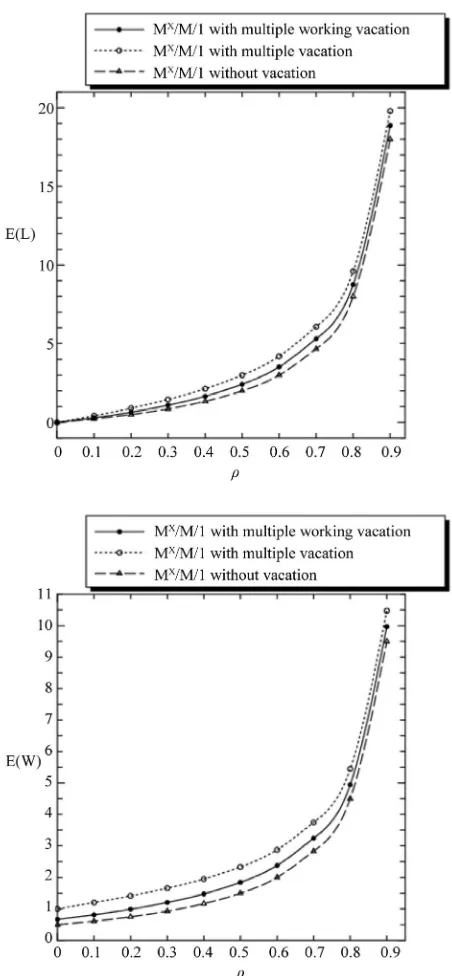
Thirdly, in Figure 3, we present the comparison of three queueing model, that is, the MX/M/1 queue without
vacation, the MX/M/1 queue with multiple vacation and
the MX/M/1 queue with multiple working vacation.
Assume that g= 2, = 2, = 1, = 1
( )
E L E W( )
for the MX/M/1
queue with multiple working vacation. Figure 3 indi-
cates that and increase as increases.
On the other hand, ( ) and of MX/M/1 queue
E L E W( )
Figure 1. E(L) versus v for different g.
Figure 2. E(L) versus v for different θ.
without vacation are shortest and those of the MX/M/1
queue with multiple vacation are longest, which is iden- tical with the intuition. Furthermore, Figure 3 indicates
that and li , which is
a well known result for batch arrival queues. 0 0 ( ) > 0 E W
( ) = 0
E L m
lim
6. Conclusion
This paper studied the MX/M/1queue with multiple
working vacation. We obtained the PGF of the stationary system length distribution and the stochastic decompo- sition structure of system length which indicates the re- lationship with that of the MX/M/1 queue without va-
cation. Performance indices such as the mean of sta- tionary system length, the probability that the system is
Figure 3. E(L) and E(W) versus ρ for different queueing model.
in a working vacation period and the probability that the system is in a regular busy period were also presented. Further, we obtained the LST of the stationary waiting time distribution of anarbitrary customer.We obtained the mean system length and the mean waiting time. Some numerical results for special cases showed efficiency of service in this multi-purpose batch arrival model.
7. Acknowledgements
[image:7.595.86.262.170.527.2]Copyright © 2012 SciRes. AJOR
ments.
REFERENCES
[1] H. Takagi, “Queueing Analysis: A Foundation of Per-formance Evaluation, Vol. 1: Vacation and Priority Sys-tems, Part 1,” Elsevier Science Publishers, Amsterdam, 1991.
[2] N. Tianand and G. Zhang, “Vacation Queueing Models- Theory and Applications,” Springer-Verlag, New York, 2006.
[3] B. Doshi, “Queueing Systems with Vacations—A Sur-vey,” Queueing Systems, Vol. 1, No. 1, 1986, pp. 29-66. doi:10.1007/BF01149327
[4] L. Servi and S. Finn, “M/M/1 Queue with Working Vaca-tions (M/M/1/WV),” Performance Evaluation, Vol. 50, No. 1, 2002, pp. 41-52.
doi:10.1016/S0166-5316(02)00057-3
[5] D. Wuand and H. Takagi, “M/G/1 Queue with Multiple Working Vacations,” Performance Evaluation, Vol. 64, 2006, pp. 654-681.
[6] Y. Baba, “Analysis of a GI/M/1 Queue with Multiple Working Vacations,” Operations Research Letters, Vol. 33, No. 2, 2005, pp. 201-209.
doi:10.1016/j.orl.2004.05.006
[7] A. Banik, U. Gupta and S. Pathak, “On the GI/M/1/N Queue with Multiple Working Vacations-Analytic Analy-sis and Computation,” Applied Mathematical Modelling, Vol. 31, No. 9, 2007, pp. 1701-1710.
doi:10.1016/j.apm.2006.05.010
[8] W. Liu, X. Xu and N. Tian, “Some Results on the M/M/1 Queue with Working Vacations,” Operations Research Letters, Vol. 35, No. 5, 2007, pp. 595-600.
doi:10.1016/j.orl.2006.12.007
[9] J. Li, N. Tian, Z. G. Zhang and H. P. Lu, “Analysis of the M/G/1 Queue with Exponential Working Vacations-A Matrix Analytic Approach,” Queueing Systems, Vol. 61, No. 2-3, 2009, pp. 139-166.
doi:10.1007/s11134-008-9103-8
[10] X. Xu, Z. Zhang and N. Tian, “Analysis for the M[X]/M/1
Working Vacation Queue,” International Journal of In-formation and Management Sciences, Vol. 20, 2009, pp. 379-394.
[11] M. F. Neuts, “Structured Stochastic Matrices of M/G/1 Type and Their Applications,” MarcelDekker Inc., New York, 1989.