© 2019, IRJET | Impact Factor value: 7.211 | ISO 9001:2008 Certified Journal
| Page 2886
Wavelet based Galerkin Method for the Numerical Solution of One
Dimensional Partial Differential Equations
S.C. Shiralashetti
1, L.M. Angadi
2, S. Kumbinarasaiah
31
Professor, Department of Mathematics, Karnatak University Dharwad-580003, India
2Asst. Professor, Department of Mathematics, Govt. First Grade College, Chikodi – 591201, India
3
Asst. Professor, Department of Mathematics, Karnatak University Dharwad-580003, India
---***---Abstract -
In this paper, we proposed the Wavelet based Galerkin method for numerical solution of one dimensional partial differential equations using Hermite wavelets. Here, Hermite wavelets are used as weight functions and these are assumed bases elements which allow us to obtain the numerical solutions of the partial differential equations. Some of the test problems are given to demonstrate the numerical results obtained by proposed method are compared with already existing numerical method i.e. finite difference method (FDM) and exact solution to check the efficiency and accuracy of the proposed methodKey Words:
Wavelet; Numerical solution; Hermite bases; Galerkin method; Finite difference method.
1.
INTRODUCTION
Wavelet analysis is newly developed mathematical tool and have been applied extensively in many engineering fileld. This has been received a much interest because of the comprehensive mathematical power and the good application potential of wavelets in science and engineering problems. Special interest has been devoted to the construction of compactly supported smooth wavelet bases. As we have noted earlier that, spectral bases are infinitely differentiable but have global support. On the other side, basis functions used in finite-element methods have small compact support but poor continuity properties. Already we know that, spectral methods have good spectral localization but poor spatial localization, while finite element methods have good spatial localization, but poor spectral localization. Wavelet bases perform to combine the advantages of both spectral and finite element bases. We can expect numerical methods based on wavelet bases to be able to attain good spatial and spectral resolutions. Daubechies [1] illustrated that these bases are differentiable to a certain finite order. These scaling and corresponding wavelet function bases gain considerable interest in the numerical solutions of differential equations since from many years [2–4].
Wavelets have generated significant interest from both theoretical and applied researchers over the last few decades. The concepts for understanding wavelets were provided by Meyer, Mallat, Daubechies, and many others, [5]. Since then, the number of applications where wavelets have been used has exploded. In areas such as approximation theory and numerical solutions of differential equations, wavelets are recognized as powerful weapons not just tools.
In general it is not always possible to obtain exact solution of an arbitrary differential equation. This necessitates either discretization of differential equations leading to numerical solutions, or their qualitative study which is concerned with deduction of important properties of the solutions without actually solving them. The Galerkin method is one of the best known methods for finding numerical solutions of differential equations and is considered the most widely used in applied mathematics [6]. Its simplicity makes it perfect for many applications. The wavelet-Galerkin method is an improvement over the standard Galerkin methods. The advantage of wavelet-Galerkin method over finite difference or finite element method has lead to tremendous applications in science and engineering. An approach to study differential equations is the use of wavelet function bases in place of other conventional piecewise polynomial trial functions in finite element type methods.
In this paper, we developed Hermite wavelet-Galerkin method (HWGM) for the numerical solution of differential equations. This method is based on expanding the solution by Hermite wavelets with unknown coefficients. The properties of Hermite wavelets together with the Galerkin method are utilized to evaluate the unknown coefficients and then a numerical solution of the one dimensional partial differential equation is obtained.
© 2019, IRJET | Impact Factor value: 7.211 | ISO 9001:2008 Certified Journal
| Page 2887
2.
PRELIMINARIES
OF HERMITE WAVELETS
Wavelets form a family of functions which are generated from dilation and translation of a single function which is called as mother wavelet
( )
x
. If the dialation parametera
and translation parameterb
varies continuously, we have the following family of continuous wavelets [7 , 8]:1/2
,
( ) =| |
(
),
,
,
0.
a b
x b
x
a
a b
R
a
a
If we restrict the parameters
a
andb
to discrete values asa
=
a
0k,
b
=
nb a
0 0k,
a
0> 1,
b
0> 0.
We have the following family of discrete wavelets1/2
0 0
, ( ) = | |
(
k),
,
,
0,
k n
x
a
a x nb
a b
R a
where
k,
n form a wavelet basis for(
)
2
R
L
. In particular, whena
0=
2
andb
0=
1
,then
k,
n(
x
)
forms an orthonormal basis. Hermite wavelets are defined as2
2 1
(2 2 1), <
, ( ) = 1 1
2 2 0, otherwise n m k n n k
H x n x
x m k k
(2.1)Where Hm 2 Hm( )x
(2.2)
where
m
=
0,1,
,
M
1.
In eq. (2.2) the coefficients are used for orthonormality. HereH
m(x
)
are the second Hermite polynomials of degree m with respect to weight function 21
=
)
(
x
x
W
on the real lineR
and satisfies the following reccurence formulaH
0(
x
)
=
1
,H
1(
x
)
=
2
x
,
H
m
2
( ) = 2
x
xH
m
1
( ) 2(
x
m
1)
H
m
( )
x
, wherem
=
0,1,2,
. (2.3)For
k
1
&
n
1
in (2.1) and (2.2), then the Hermite wavelets are given by1,0
2
( )
x
,1,1
2
( )
x
( 4
x
2)
, 2 1,22
( )
x
(16
x
16
x
2 )
, 3 2 1,32
( )
x
(64
x
96
x
36
x
2 )
,4 3 2
1,4
2
( )
x
(256
x
512
x
320
x
64
x
2 )
, and so on.Function approximation:
We would like to bring a solution function
u x
( )
under Hermite space by approximatingu x
( )
by elements of Hermite wavelet bases as follows,, ,
1 0( )
n m n m n mu x
c
x
© 2019, IRJET | Impact Factor value: 7.211 | ISO 9001:2008 Certified Journal
| Page 2888
where
n m,
x
is given in eq. (2.1).We approximate
u x
( )
by truncating the series represented in Eq. (2.4)as,
1 1 2 , , 1 0( )
k Mn m n m n m
u x
c
x
(2.5)where
c
and
are2
k
1
M
1
matrix.Convergence of Hermite wavelets
Theorem: If a continuous function
2
u x
L R
defined on
0 , 1
be bounded, i.e.u x
K
, then the Hermitewavelets expansion of
u x
converges uniformly to it [9].Proof: Let
u x
be a bounded real valued function on
0 , 1
. The Hermite coefficients of continuous functionsu x
is defined as,
1
, ,
0
n m n m
C
u x
x dx
1 2
2
2
2
1
k
k m I
u x
H
x
n
dx
, where1
1,
12
k2
kn
n
I
Put
2
kx
2
n
1
z
1 1 2
1
2
1
2
2
2
k k m kz
n
u
H
z
dx
1 1 2 12
1
2
2
km k
z
n
u
H
z dx
Using GMVT integrals,
1
1 2
1
2
1
2
2
km k
w
n
u
H
z dx
, for somew
1,1
1 2
2
1
2
2
k kw
n
u
h
where
1
1
m
h
H
z dx
1 2 ,2
1
2
2
k
n m k
w
n
C
u
h
Since
u
is bounded, therefore ,, 0 n m n m
C
absolutely convergent. Hence the Hermite series expansion ofu x
© 2019, IRJET | Impact Factor value: 7.211 | ISO 9001:2008 Certified Journal
| Page 2889
3.
METHOD OF SOLUTION
Consider the differential equation of the form,
u
f
x
x
u
x
u
2 2 (3.1)With boundary conditions
u
0
a
,
u
1
b
(3.2) Where
,
are may be constant or either a functions ofx
or functions ofu
andf
x
be a continuous function.Write the equation (3.1) as
u
f
x
x
u
x
u
x
R
2 2
)
(
(3.3)where
R
x
is the residual of the eq. (3.1). WhenR
x
0
for the exact solution,u x
( )
only which will satisfy the boundary conditions.Consider the trail series solution of the differential equation (3.1),
u x
( )
defined over [0, 1) can be expanded as a modified Hermite wavelet, satisfying the given boundary conditions which is involving unknown parameter as follows,
1 1 2 , , 1 0( )
k Mn m n m n m
u x
c
x
(3.4)where
c
n m,'
s
are unknown coefficients to be determined.Accuracy in the solution is increased by choosing higher degree Hermite wavelet polynomials.
Differentiating eq. (3.4) twice with respect to
x
and substitute the values of2
2
,
,
u
u
u
x
x
in eq. (3.3). To findc
n m,'
s
wechoose weight functions as assumed bases elements and integrate on boundary values together with the residual to zero [10]. i.e. 1
1, 0
0
m x R x dx
,m
0, 1, 2,...
then we obtain a system of linear equations, on solving this system, we get unknown parameters. Then substitute these unknowns in the trail solution, numerical solution of eq. (3.1) is obtained.
4.
NUMERICAL EXPERIMENT
Test Problem 4.1 First, consider the differential equation [11],
2
2
, 0
1
u
u
x
x
x
(4.1)With boundary conditions:
u
0
0,
u
1
0
(4.2) The implementation of the eq. (4.1) as per the method explained in section 3 is as follows:The residual of eq. (4.1) can be written as:
2 2
u
R x
u
x
x
(4.3)Now choosing the weight function
w x
x
(1
x
)
for Hermite wavelet bases to satisfy the given boundary conditions(4.2), i.e.
ψ
x
w x
x
( )
x
1,0( )
x
x
(1
x
)
2
x
(1
x
)
1,0
ψ
,1,1
( )
x
1,1( )
x
x
(1
x
)
2
( 4
x
2) (1
x
x
)
ψ
2
1,2 1,2 (1 )
2
( )
x
( )
x
x x(16
x
16
x
2 ) (1
x
x
)
© 2019, IRJET | Impact Factor value: 7.211 | ISO 9001:2008 Certified Journal
| Page 2890
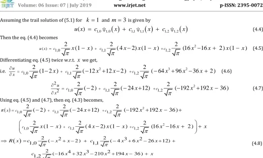
Assuming the trail solution of (5.1) fork
1
andm
3
is given by
u x
( )
c
1,0ψ
1,0
x
c
1,1ψ
1,1
x
c
1,2ψ
1,2
x
(4.4) Then the eq. (4.4) becomes2
( ) 1,0
2
(1
)
1,12
( 4
2) (1
)
1,22
(16
16
2 ) (1
)
u x c
x
x
cx
x
x
cx
x
x
x
(4.5)Differentiating eq. (4.5) twice w.r.t.
x
we get,i.e. 2 3 2
1,0 1,1 1,2
2
2
2
(1 2 )
( 12
12
2 )
( 64
96
36
2 )
c c c
u
x
x
x
x
x
x
x
(4.6)2
1,0 1,1 1,2
2
2
2
2
2
( 2 )
( 24
12)
( 192
192
36 )
c c c
u
x
x
x
x
(4.7)Using eq. (4.5) and (4.7), then eq. (4.3) becomes,
2
2
1,0 1,1 1,2
1,0 1,1 1,2
2
2
2
( 2 )
(
24
12)
( 192
192
36 )
2
2
2
(1
)
( 4
2) (1
)
(16
16
2 )
R c c c
c c c
x
x
x
x
x
x
x
x
x
x
x
x
2 ( 2 2 ) 2 ( 4 3 6 2 26 12)1,0 1,1
2 4 3 2
( 16 32 210 194 36 )
1,2
R x c x x c x x x
c x x x x x
(4.8)
This is the residual of eq. (4.1). The “weight functions” are the same as the bases functions. Then by the weighted Galerkin method, we consider the following:
1
1, 0
0
m
x R x dx
,m
0, 1 , 2
(4.9) Form
0, 1, 2
in eq. (4.9),i.e.
1 1,0 0
0
x R x dx
,
1 1,1 00
x R x dx
,
1 1, 2 00
x R x dx
( 0.3802)
c
1,1
(0)
c
1,2
(0.4487)
c
1,3
0.0940
0
(4.10)1,1 1,2 1,3
(0)
c
(0.9943)
c
(0)
c
0.0376
0
(4.11)1,0 1,1 1,2
(0.4487)
c
(0)
c
(2.3686)
c
0.1128
0
(4.12) We have three equations (4.10) – (4.12) with three unknown coefficients i.e.c
1,0 ,c
1,1 andc
1,2 . By solving this system of algebraic equations, we obtain the values ofc
1,0
0.2446
,c
1,1
0.0378
andc
1,2
0.0013
. Substituting these values in eq. (4.5), we get the numerical solution; these results and absolute error =u
a
x
u
e
x
(whereu
a
x
andu x
e
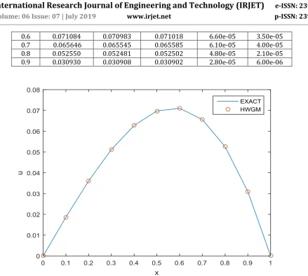
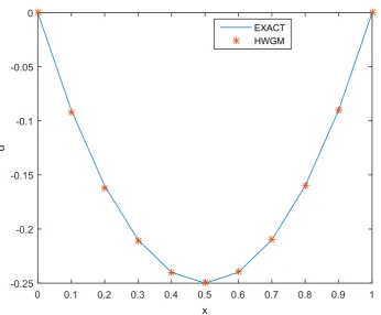
are numerical and exact solutions respectively) are presented in table - 1 and fig - 1 in comparison with exact solution of eq. (4.1) issin ( )
( )
sin (1)
x
[image:5.595.36.559.61.375.2]u x
x
.Table – 1: Comparison of numerical solution and exact solution of the test problem 4.1
x Numerical solution Exact solution Absolute error
FDM HWGM FDM HWGM
© 2019, IRJET | Impact Factor value: 7.211 | ISO 9001:2008 Certified Journal
| Page 2891
0.6 0.071084 0.070983 0.071018 6.60e-05 3.50e-05 [image:6.595.81.521.48.442.2]0.7 0.065646 0.065545 0.065585 6.10e-05 4.00e-05 0.8 0.052550 0.052481 0.052502 4.80e-05 2.10e-05 0.9 0.030930 0.030908 0.030902 2.80e-05 6.00e-06
Fig – 1: Comparison of numerical and exact solutions of the test problem 4.1.
Test Problem 4.2 Next, consider another differential equation [12]
2
2 2
2
2
sin
, 0
1
u
u
x
x
x
(4.12)With boundary conditions:
u
0
0,
u
1
0
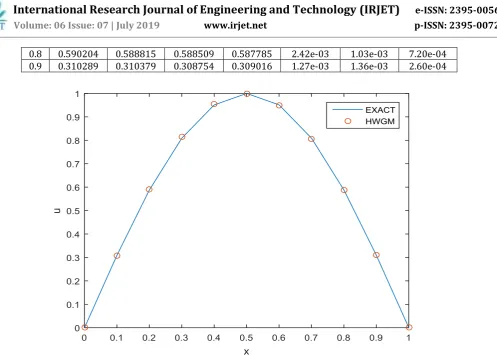
(4.13) Which has the exact solutionu x
sin
x
.By applying the method explained in the section 3, we obtain the constants
c
1,0
3.1500
,c
1,1
0
andc
1,2
0.1959
. Substituting these values in eq. (4.5) we get the numerical solution. Obtained numerical solutions are compared with exact and other existing method solutions are presented in table - 2 and fig - 2.Table – 2: Comparison of numerical solution and exact solution of the test problem 4.2.
x Numerical solution solution Exact Absolute error
FDM Ref [11] HWGM FDM Ref [11] HWGM
[image:6.595.62.541.641.792.2]© 2019, IRJET | Impact Factor value: 7.211 | ISO 9001:2008 Certified Journal
| Page 2892
0.8 0.590204 0.588815 0.588509 0.587785 2.42e-03 1.03e-03 7.20e-04 [image:7.595.58.556.46.407.2]0.9 0.310289 0.310379 0.308754 0.309016 1.27e-03 1.36e-03 2.60e-04
Fig – 2: Comparison of numerical and exact solutions of the test problem 4.2.
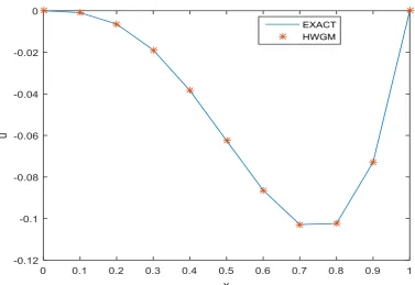
Test Problem 4.3 Consider another differential equation [13]
2
1
2
1 , 0
1
x
u
u
e
x
x
x
(4.14)With boundary conditions:
u
0
0,
u
1
0
(4.15) Which has the exact solution
1
1
xu x
x
e
.By applying the method explained in the section 3, we obtain the constants
c
1,0
0.7103
,c
1,1
0.0806
andc
1,2
0.0064
. Substituting these values in eq. (4.5) we get the numerical solution. Obtained numerical solutions are compared with exact and other existing method solutions are presented in table - 3 and fig - 3.Table - 3: Comparison of numerical solution and exact solution of the test problem 4.3.
x Numerical solution solution Exact Absolute error
FDM Ref [12] HWGM FDM Ref [12] HWGM
[image:7.595.83.512.596.745.2]© 2019, IRJET | Impact Factor value: 7.211 | ISO 9001:2008 Certified Journal
| Page 2893
Fig – 3: Comparison of numerical and exact solutions of the test problem 4.3.
Test Problem 4.4 Now, consider singular boundary value problem [12]
2
2
2 2
2
2
4
, 0
1
u
u
u
x
x
x
x
x
x
(4.16)With boundary conditions:
u
0
0,
u
1
0
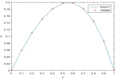
(4.17) Which has the exact solution
2u x
x
x
.By applying the method explained in the section 3, we obtain the constants
c
1,0
0.8945
,c
1,1
0.0047
and1,2
0.0046
c
. Substituting these values in eq. (4.5) we get the numerical solution. Obtained numerical solutions are compared with exact and other existing method solutions are presented in table - 4 and fig - 4.Table - 4: Comparison of numerical solution and exact solution of the test problem 4.4.
x Numerical solution Exact solution Absolute error
FDM HWGM FDM HWGM
[image:8.595.99.499.570.707.2]© 2019, IRJET | Impact Factor value: 7.211 | ISO 9001:2008 Certified Journal
| Page 2894
Fig – 4: Comparison of numerical solution and exact solution of the teat problem 4.4.
Test Problem 4.5 Finally, consider another singular boundary value problem [14]
2
5 4 2
2
8
44
30 , 0
1
u
u
x u
x
x
x
x
x
x
x
x
(4.16)With boundary conditions:
u
0
0,
u
1
0
(4.17) Which has the exact solution
3 4u x
x
x
.By applying the method explained in the section 3, we obtain the constants and substituting these values in eq. (4.5) we get the numerical solution. Obtained numerical solutions are compared with exact and other existing method solutions are presented in table - 5 and fig - 5.
Table – 5: Comparison of numerical solution and exact solution of the test problem 4.5.
x Numerical solution Exact solution Absolute error
FDM HWGM FDM HWGM
[image:9.595.113.483.579.716.2]© 2019, IRJET | Impact Factor value: 7.211 | ISO 9001:2008 Certified Journal
| Page 2895
Fig - 5: Comparison of numerical solution and exact solution of the teat problem 4.5.
5.
CONCLUSIONIn this paper, we proposed the wavelet based Galerkin method for the numerical solution of one dimensional partial differential equations using Hermite wavelets. The efficiency of the method is observed through the test problems and the numerical solutions are presented in Tables and figures, which show that HWGM gives comparable results with the exact solution and better than existing numerical methods. Also increasing the values of
M
, we get more accuracy in the numerical solution. Hence the proposed method is effective for solving differential equations.References
[1] I. Daubechie, Orthonormal bases of compactly supported wavelets, Commun. Pure Appl. Math., 41(1988), 909-99.
[2] S. C. Shiralashetti, A. B. Deshi, “Numerical solution of differential equations arising in fluid dynamics using Legendre wavelet collocation method”, International Journal of Computational Material Science and Engineering, 6 (2), (2017) 1750014 (14 pages).
[3] S. C. Shiralashetti, S. Kumbinarasaiah, R. A. Mundewadi, B. S. Hoogar, Series solutions of pantograph equations using wavelets, Open Journal of Applied & Theoretical Mathematics, 2 (4) (2016), 505-518.
[4] K. Amaratunga, J. R. William, Wavelet-Galerkin Solutions for One dimensional Partial Differential Equations, Inter. J. Num. Meth. Eng., 37(1994), 2703-2716.
[5] I. Daubeshies, Ten lectures on Wavelets, Philadelphia: SIAM, 1992.
[6] J. W. Mosevic, Identifying Differential Equations by Galerkin's Method, Mathematics of Computation, 31(1977), 139-147.
[7] A. Ali, M. A. Iqbal, S. T. Mohyud-Din, Hermite Wavelets Method for Boundary Value Problems, International Journal of Modern Applied Physics, 3(1) (2013), 38-47 .
© 2019, IRJET | Impact Factor value: 7.211 | ISO 9001:2008 Certified Journal
| Page 2896
[9] R. S. Saha, A. K. Gupta, A numerical investigation of time fractional modified Fornberg-Whitham equation for analyzingthe behavior of water waves. Appl Math Comput 266 (2015),135–148
[10] J. E. Cicelia, Solution of Weighted Residual Problems by using Galerkin’s Method, Indian Journal of Science and Technology,7(3) (2014), 52–54.
[11] S. C. Shiralashetti, M. H. Kantli, A. B. Deshi, A comparative study of the Daubechies wavelet based new Galerkin and Haar wavelet collocation methods for the numerical solution of differential equations, Journal of Information and Computing Science, 12(1) (2017), 052-063.
[12] T. Lotfi, K. Mahdiani, Numerical Solution of Boundary Value Problem by Using Wavelet-Galerkin Method, Mathematical Sciences, 1(3), (2007), 07-18.
[13] J. Chang, Q. Yang, L. Zhao, Comparison of B-spline Method and Finite Difference Method to Solve BVP of Linear ODEs , Journal of Computers, 6 (10) (2011), 2149-2155.
[14] V. S. Erturk, Differential transformation method for solving differential equations of lane-emden type, Mathematical and Computational Applications, 12(3) (2007), 135-139.
BIOGRAPHIES
Dr. S. C. Shiralashetti was born in 1976. He received M.Sc., M.Phil, PGDCA, Ph.D. degree, in Mathematics from Karnatak University, Dharwad. He joined as a Lecturer in Mathematics in S. D. M. College of Engineering and Technology, Dharwad in 2000 and worked up to 2009. Futher, worked as a Assistant professor in Mathematics in Karnatak College Dharwad from 2009 to 2013, worked as a Associate Professor from 2013 to 2106 and from 2016 onwards working as Professor in the P.G. Department of studies in Mathematics, Karnatak University Dharwad. He has attended and presented more than 35 research articles in National and International conferences. He has published more than 36 research articles in National and International Journals and procedings.
Area of Research: Numerical Analysis, Wavelet Analysis, CFD, Differential Equations, Integral Equations, Integro-Differential Eqns.
H-index: 09; Citation index: 374.
Dr. Kumbinarasaiah S, received his B.Sc., degree (2011) and M.Sc., degree in Mathematics (2013) from Tumkur University, Tumkur. He has cleared both CSIR-NET (Dec 2013) and K-SET (2013) in his first attempt. He received Ph.D., in Mathematics (2019) at the Department of Mathematics, Karnatak University, Dharwad. He started his teaching career from September 2014 as an Assistant Professor at Department of Mathematics, Karnatak University, Dharwad.
Area of research:Linear Algebra, Differential Equations, Wavelet theory, and its applications. H-index: 03; Citation index: 23
2
ndAuthor
Photo
1’st
Author
Photo
Dr. L. M. Angadi, received M.Sc., M.Phil, Ph.D. degree, in Mathematics from Karnatak University, Dharwad. In September 2009, he joined as Assistant Professor in Govt. First Grade College, Dharwad and worked up
to August 2013 and september 2013 onwards working in Govt. First Grade College, Chikodi (Dist.: Belagavi).