Feature-Rich Error Detection in Scientific Writing
Using Logistic Regression
Madeline Remse, Mohsen Mesgar and Michael Strube Heidelberg Institute for Theoretical Studies gGmbH
Schloß-Wolfsbrunnenweg 35 69118 Heidelberg, Germany
(madeline.remse|mohsen.mesgar|michael.strube)@h-its.org
Abstract
The goal of the Automatic Evaluation of Sci-entific Writing (AESW) Shared Task 2016 is to identify sentences in scientific articles which need editing to improve their correct-ness and readability or to make them better fit within the genre at hand. We encode many dif-ferent types of errors occurring in the dataset by linguistic features. We use logistic regres-sion to assign a probability indicating whether a sentence needs to be edited. We participate in both tracks at AESW 2016: binary pre-diction and probabilistic estimation. In the former track, our model (HITS) gets the fifth place and in the latter one, it ranks first accord-ing to the evaluation metric.
1 Introduction
The AESW 2016 Shared Task is about predicting if a given sentence in a scientific article needs lan-guage editing. It can therefore be pictured as a bi-nary classification task. Two types of prediction are evaluated: binary prediction (falseortrue) and prob-abilistic estimation (between 0 and 1). These types of prediction form the two tracks of the shared task, both of which we participate in.
We solve both problems by applying a logistic regression model. We design a variety of features based on a thorough analysis of the training data. We choose the set of features that yields the highest performance on training and development sets.
Accounting for the imbalance of numbers of wrong and correct sentences in the training data dur-ing feature selection we obtain a model for the prob-abilistic task that outranks our competitors’ systems.
However, a detailed analysis of the results shows that the model takes advantage of the evaluation metric and that our less informed system produces results that are, although not yielding a top evalua-tion score, more meaningful.
In the course of a profound analysis of the train-ing data we encounter both ltrain-inguistic errors, which likely occur in diverse genres, and such errors that are intrinsic to scientific writing and thus rank among the major challenges of this task. As pointed out on the AESW 2016 webpage1, correcting prob-lems concerning diction and style is a matter of opin-ion. It depends on factors that are not necessarily deducible from linguistic properties. Common ab-breviations are an example. There are cases where they are accepted by an editor, and there are cases where they are corrected. That is, sometimese.g.is left as is and sometimes it is changed tofor instance orfor examplewithout any obvious reason. There are even words that are corrected in opposite direc-tions. For example, the first letter of the name prefix vanhas been corrected to be uppercase in some sen-tences and also has been corrected to be lowercase in other sentences. Especially abbreviations that are not common within one particular domain, but are used in isolated documents are problematic. This is due to limitations of the dataset, which provides only paragraphs, but not documents as contexts for sen-tences. For example, we may assume thatR-Ghas been introduced as a technical term at some point in a document. But since we do not know which para-graphs belong to this document, we cannot be sure that this is the case.
1http://textmining.lt/aesw/index.html
Section 2 gives an overview of the types of errors we encountered. In Section 3 we introduce our sys-tem design, detail on how we derive features from our data analysis, what kinds of language models we apply, give a short outline on logistic regression and describe the implementation of our system. In Sec-tion 4 we describe our training steps, followed by re-porting results in Section 5, a discussion of lessons learned in Section 6 and related work in Section 7.
2 Data Analysis2
2.1 Simple Errors
SPELLING ERRORS are frequent and many con-cern using hyphens in compounds. Another com-mon error is the wrong usage of ARTICLES. Def-inite articles are missing or unnecessarily inserted before generic nouns, (for instance over the for-mula REF ). Indefinite articles are erroneous with respect to the subsequent phoneme, (e.g. a open neighborhood). Some errors concern descrip-tions of REFERENCES, which are usually capital-ized (table REF or figures REF and REF ). NUMERALS are spelled out when they should not be, and vice-versa (2 or seventy-three). It is correct to spell numerals out if they are smaller than 10, otherwise they are often spelled in dig-its. CONTRACTIONS, such as doesn’t and what’s, are considered too colloquial for scientific writ-ing. Dots behind ABBREVIATIONSare omitted, and also common abbreviations such as e.g., i.e. and vs. are written wrongly. Other errors include in-correct PLURALIZATION of decades (1980’s), reg-ular past tense generation of IRREGULAR VERBS (lighted) and the modification of words by the wrong PREPOSITION (very different to the
correc-tion). Words are unnecessarily REPEATED some-times (The the).
2.2 Complex Errors
All errors described above can easily be categorized by means of simple patterns. Other errors are harder to capture, for example wrong word order or miss-ing words. The most common errors that we come across are mistakes in the PUNCTUATIONof a sen-tence, especially unnecessary or missing commas.
2All examples in this section have been drawn from the training data.
NUMBER DISAGREEMENT is a common gram-matical error. It occurs in passive or active clauses (e.g. the system are assumed to be the following form and the counter variables goes on changing) and in nominal phrases (e.g.Three class of boundary conditionsandthese new set of Lyapunov terms).
WORK-SPECIFIC ABBREVIATIONS such as the insertion ofR-G for the compound recombination-generationare errors that occur in individual situa-tions. Detecting issues withDICTION AND STYLEis probably the most intricate problem in this task.
3 System Design
3.1 Formally Capturing Error Types
Simple errors can mostly be captured by binary fea-tures that formalize rules. For example, if a sentence contains an incorrectABBREVIATIONofid est, such as ie., then it needs correction. Similar rules can be applied to the spelling mode of cardinal numbers and theCONTRACTIONof auxiliary words, such as
’s, ’ve, etc. Also, when finding a four digit num-ber starting with1and ending with0, it is likely to denote a decade. If it is directly followed by’s, an incorrectPLURALIZATIONis detected.
Some rules formulated that way need additional information. To assert that seventeen should not be spelled out the system must be aware that it de-notes a NUMERAL greater than 10. This informa-tion can be made available through appropriate map-pings. Lists of wrongly generated past tense forms of IRREGULAR VERBS can be created with man-agable effort, just like lists of common abbrevia-tions.
SPELLING ERRORScan be detected by looking up words in a dictionary. Whether or not a compound requires being joined by a hyphen cannot be deter-mined that way. Compounds can be created produc-tively and are not necessarily in a dictionary.
NUMBER DISAGREEMENTSare easy to detect by means of dependencies between head and modifiers within phrases and part-of-speech tags, which often carry information about the number of words. How-ever, that means that recognizing these errors heav-ily depends on the correctness of the dependency trees and the part-of-speech tags.
combination with the same words. Thus an appro-priately trained language model learns that the word different occurs with from much more frequently than withto. Classic n-gram models account for un-usual sequences of words and faulty word orderings. Language models based on co-occurrences of con-stituents in syntax trees can reveal grammatical er-rors and indicate positions where a comma or article is likely to be inserted.
3.2 Language Models
To capture more complex errors we use a variety of language models that we compute on correct sen-tences in the training data.
The n-gram probability of the ith linguistic unit
of a sentenceli, being a tokenwor a part-of-speech
tagt, given itsn−1predecessors is defined as
p(li |lii−−1n+1) = c(l i i−n+1)
c(lii−−1n+1),
where c(x) is the number of occurrences of x throughout the dataset (Jurafsky and Martin, 2009, pp. 117–147).
Language modeling is not limited to a language unit and its direct predecessors. The probability of the occurrence of a word or part-of-speech tag can be computed depending on whatever might be ap-propriate to model a linguistic phenomenon. There-fore we compute the probability of a linguistic unit given the subsequentn−1linguistic units:
p(li |lii++1n−1) = c(l
i+n−1
i )
c(li+n−1
i+1 )
.
The following formula for the probability of a word waccounts for the relation between part-of-speech tags and lexicals:
p(wi |ti) = c(cw(it, ti) i) .
In order to identify words that are typically preceded by a particular part-of-speech, we compute
p(ti |wi+1) = c(ct(iw, wi+1)
i+1) .
Given a syntax tree, letsucc(g)be the right sibling of a nodeg, letpred(g)be the left sibling of a node
g, and letchild(g)be the set of children of a nodeg. We define:
p(pred(h) =g|h) = P c(pred(h) =g)
g0∈Cc(pred(h) =g0),
p(succ(h) =g|h) = P c(succ(h) =g)
g0∈Cc(pred(h) =g0),
p(g∈child(h)|h) = P c(g∈child(h))
g0∈Cc(g0 ∈child(h)),
whereCis the set of constituents.
Other sets of features address the probability of prepositional phrases as modifiers of words. Let nmod(v)be a preposition that modifies a wordv:
p(nmod(v) =w) = P c(nmod(v) =w)
w0∈V c(nmod(v) =w0).
Smoothing: Since the purpose of our language models is to identify unusual combinations and or-derings of words, part-of-speech tags, and chunks, we go without strong smoothing measures and leave it to machine learning to reveal the point where a language construct qualifies as unacceptably im-probable. Also, we do not prune the vocabulary, be-cause technical terms which are limited to very spe-cific scientific fields or even to only few documents are characteristic for scientific writing. For practi-cal reasons we apply the very basic add-δ smooth-ing (Jurafsky and Martin, 2009, p. 134), choossmooth-ing δ= 0.1in order to prevent zero-division.
3.3 Features
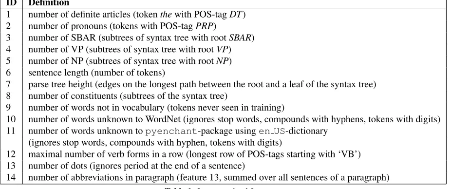
We implement a total of 82 features based on the data analysis described in Section 2. These fea-tures can be classified into three sets, depending on their range. Features 1–14 (see Table 1) are integer-valued, features 15–55 (see Table 2) are binary, and features 56–82 (see Table 3) are real-valued.
ID Definition
1 number of definite articles (tokenthewith POS-tagDT) 2 number of pronouns (tokens with POS-tagPRP)
3 number of SBAR (subtrees of syntax tree with rootSBAR) 4 number of VP (subtrees of syntax tree with rootVP) 5 number of NP (subtrees of syntax tree with rootNP) 6 sentence length (number of tokens)
7 parse tree height (edges on the longest path between the root and a leaf of the syntax tree) 8 number of constituents (subtrees of the syntax tree)
9 number of words not in vocabulary (tokens never seen in training)
10 number of words unknown to WordNet (ignores stop words, compounds with hyphens, tokens with digits) 11 number of words unknown topyenchant-package usingen US-dictionary
(ignores stop words, compounds with hyphen, tokens with digits)
12 maximal number of verb forms in a row (longest row of POS-tags starting with ‘VB’) 13 number of dots (ignores period at the end of a sentence)
[image:4.612.75.538.64.258.2]14 number of abbreviations in paragraph (feature 13, summed over all sentences of a paragraph)
Table 1:Integer-valued features.
occur in too complex sentences. Many pronouns are indicative for ambiguity, since it is more difficult to identify the corresponding antecedents.
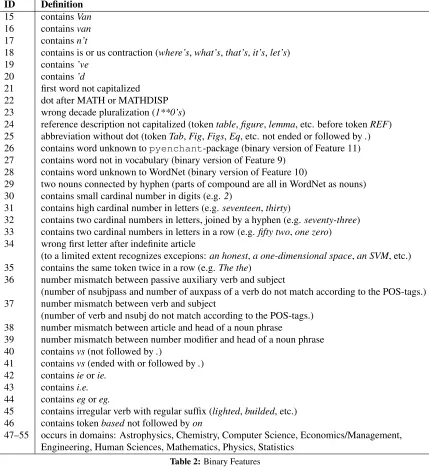
The binary features are mostly designed for spe-cific error types, looking for patterns or exact strings found to be frequently corrected in the training data. Abbreviations sometimes are and sometimes are not accepted (Section 2). In order to capture more information on their usage we added Features 13 and 14. They count the number of abbreviations in the sentence and in the whole paragraph respectively. The general idea is that if an author has a tendency to use abbreviations, an editor does not perceive an individual abbreviation as inconsistent.
Features 47–55 recognize domain-related errors. Although the domain is unlikely to be directly de-cisive for distinguishing correct from incorrect sen-tences, some kinds of errors might coincide with in-dividual domains. Our model does not take into ac-count dependencies between features (Jurafsky and Martin, 2009, p. 238). However we examine their impact on the model’s performance. They could be beneficial for other machine learning algorithms.
In order to detect spelling errors, some of the bi-nary features check if all words in a sentence are present within specific sets, such as the vocabu-lary used in the correct training data, an American English dictionary3, or WordNet4. We implement
3We used thepyenchantpackage: http://pythonhosted.org/pyenchant/
4https://wordnet.princeton.edu/
integer-valued counterparts for these features, be-cause an absolute decision might be too restrictive.
Most of the real-valued features consist of proba-bilities computed in our language models. We com-pute maximum likelihood estimates of sentences based on different models. We use part-of-speech n-grams and token n-grams for n ∈ {1,2,3} and a Hidden Markov Model. We also capture those n-grams in a sentence that yield the lowest proba-bility compared to all other n-grams. Furthermore there are features that detect the position where a comma is most likely to be inserted with respect to the preceding and succeeding tokens and part-of-speech tags as well as the preceding, succeed-ing and superordinate constituents in the syntax tree. The same is done for inserting and deleting articles and substituting prepositions by other prepositions. Mostly we do not compute an isolated probability, but rather connect it with comparative probabilities. For instance, feature 82 does not only compute the probability of a comma before a pair of words, but returns the factor by which a comma is more likely than the word actually preceding the pair. That way the feature does depend on the subsequent word pair and also on the word to be substituted.
3.4 Machine Learning Approach
ID Definition
15 containsVan
16 containsvan
17 containsn’t
18 contains is or us contraction (where’s,what’s,that’s,it’s,let’s) 19 contains’ve
20 contains’d
21 first word not capitalized 22 dot after MATH or MATHDISP 23 wrong decade pluralization (1**0’s)
24 reference description not capitalized (tokentable,figure,lemma, etc. before tokenREF) 25 abbreviation without dot (tokenTab,Fig,Figs,Eq, etc. not ended or followed by.) 26 contains word unknown topyenchant-package (binary version of Feature 11) 27 contains word not in vocabulary (binary version of Feature 9)
28 contains word unknown to WordNet (binary version of Feature 10)
29 two nouns connected by hyphen (parts of compound are all in WordNet as nouns) 30 contains small cardinal number in digits (e.g.2)
31 contains high cardinal number in letters (e.g.seventeen,thirty)
32 contains two cardinal numbers in letters, joined by a hyphen (e.g.seventy-three) 33 contains two cardinal numbers in letters in a row (e.g.fifty two,one zero) 34 wrong first letter after indefinite article
(to a limited extent recognizes excepions:an honest,a one-dimensional space,an SVM, etc.) 35 contains the same token twice in a row (e.g.The the)
36 number mismatch between passive auxiliary verb and subject
(number of nsubjpass and number of auxpass of a verb do not match according to the POS-tags.) 37 number mismatch between verb and subject
(number of verb and nsubj do not match according to the POS-tags.) 38 number mismatch between article and head of a noun phrase
39 number mismatch between number modifier and head of a noun phrase 40 containsvs(not followed by.)
41 containsvs(ended with or followed by.) 42 containsieorie.
43 containsi.e.
44 containsegoreg.
45 contains irregular verb with regular suffix (lighted,builded, etc.) 46 contains tokenbasednot followed byon
[image:5.612.88.517.62.529.2]47–55 occurs in domains: Astrophysics, Chemistry, Computer Science, Economics/Management, Engineering, Human Sciences, Mathematics, Physics, Statistics
Table 2:Binary Features
phase is also not very time-consuming, which is ben-eficial for our feature selection procedure. It derives the probability of an observation x to belong to a particular class y from a linear combination of the observed feature vectorf and a weight vectorw (Ju-rafsky and Martin, 2009, pp. 231–239). It applies a logistic function to map the result of this linear combination to lie between 0 and 1. In the train-ing phase the parameters in ware chosen to maxi-mize the probability of the observedyvalues. Dur-ing testDur-ing unseen samples are classified accordDur-ing to their probability computed by linearly combining
their feature vectors with the very weight vectorw that was determined in training.
3.5 Implementation
ID Definition
56 average word length
57 max. gain of changing a preposition (nmod(w)denotes preposition that modifiesw): max( pmodify(w0,wi)
pmodify(nmod(wi),wi) : 1≤i≤ |S|ANDw
0∈V AND∃j1≤j ≤ |S| ∧nmod(w
i) =wj ), 58 max. gain of swapping the case of a first letter (swap(w)iswwith case of first letter swapped)):
max(pngram(wi−2,wi−1,swap(wi))
pngram(wi−2,wi−1,wi) : 1≤i≤ |S| ),
59 maximum likelihood estimate (token unigrams):Q1≤i≤|S| p(wi) 60 maximum likelihood estimate (POS-tag unigrams):Q1≤i≤|S| p(ti) 61 maximum likelihood estimate (token bigrams):Q1≤i≤|S| p(wi |wi−1)
62 maximum likelihood estimate (POS-tag bigrams):Q1≤i≤|S| p(ti|ti−1)
63 maximum likelihood estimate (token trigrams):Q1≤i≤|S| p(wi|wi−2wi−1)
64 maximum likelihood estimate (POS-tag trigrams):Q1≤i≤|S| p(ti|ti−2ti−1)
65 maximum likelihood estimate (Hidden Markov Model):Q1≤i≤|S| p(ti|ti−1)·p(wi|ti) 66 min. probability of any POS-tag trigram:min(p(ti|ti−2ti−1) : 1≤i≤ |S| )
67 min. probability of any POS-tag bigram:min(p(ti|ti−1) : 1≤i≤ |S| )
68 min. probability of any POS-tag unigram:min(p(ti) : 1≤i≤ |S| )
69 min. probability of any token trigram:min(p(wi |wi−2wi−1) : 1≤i≤ |S| )
70 min. probability of any token bigram:min(p(wi|wi−1) : 1≤i≤ |S| )
71 min. probability of any token unigram:min(p(wi) : 1≤i≤ |S| ) 72 min. lexical probability of any token:min(p(wi|ti) : 1≤i≤ |S| ) 73 fraction of tokens that are commas: |{i:wi=,:1≤i≤|S|}|
|S|
74 max. gain of inserting comma after chunk:max(p(succ(g) =,|g) :g∈Tree(S)ANDsucc(g)6=, ) 75 max. gain of inserting comma before chunk:max(p(pred(g) =,|g) :g∈Tree(S)ANDpred(g)6=, ) 76 max. gain of inserting comma within subtree:max(p(,∈g|g) :g∈Tree(S)AND,∈/child(g) ) 77 max. gain of inserting article:max(p(DT|wi)
p(ti−1,wi) : 1≤i≤ |S|ANDti−16=DT )
78 max. gain of deleting article:max(p(ti−2,wi)
p(DT|wi) : 1≤i≤ |S|ANDti−1=DT )
79 max. gain of inserting comma after pair of POS-tags:max(p(,|ti−2ti−1)
p(ti|ti−2ti−1): 1≤i≤ |S| ) 80 max. gain of inserting comma after pair of words:max( p(,|wi−2wi−1)
p(wi|wi−2,wi−1) : 1≤i≤ |S| ) 81 max. gain of inserting comma before pair of POS-tags:max(p(,|ti+1ti+2)
p(ti|ti+1ti+2): 1≤i≤ |S| ) 82 max. gain of inserting comma before pair of words:max( p(,|wi+1wi+2)
p(wi|wi+1wi+2): 1≤i≤ |S| )
Table 3:Real-valued features
dependency relation between the corresponding to-kens. The object can hold both its correct and its incorrect versions. The Sentence class also imple-ments all features and methods needed for data anal-ysis. The purpose of the Corpus class is to gather and manipulate sentence information and transfer it to convenient output formats. It also holds a static object that encapsulates all functionality regarding language modeling.
Each step on the way to the final system is then implemented in a seperate script that accesses the data model described above. These steps can be combined to form a closed system or be extended to do further data analysis or to use machine learning approaches other than logistic regression.
For machine learning we used the
scikit-learn5 implementation of logistic regression.
4 Training
All sentences in the training set are used for train-ing, that is, a sentence that needs correction enters the training set with both its original and its cor-rected version and thus introduces two samples with different labels to the training data, namely−1 for the correct version and+1 for the wrong version. Sentences that do not need modification have the label −1. To prevent single features from being predominant we scale all feature vectors using the scikit-learn MaxAbsScaler. It maps all our
values to lie between 0 and 1 by dividing by the largest absolute value that occurs in each feature dur-ing traindur-ing. That way binary features and0values remain unaffected. Note that test data samples can still end up with feature values greater than1, but all features will still be cut to reasonable sizes.
4.1 Feature Selection
In order to determine which of the features are help-ful in an actual system, we first extract a small sub-set of binary features that all yield a high precision when classifying sentences of the development set solely based on their value. Seven of the features yield a precision of more than90%, namely 17, 18, 19, 22, 23, 32, and 42. We train a logistic regres-sion model using only these features. We evaluate the predictions of the model using the F1-scores for both tracks of the shared task, as defined in (Dau-daraviˇcius, 2015). Then we add each of the remain-ing features and keep the one that improves the F1-score most. We repeat that process until none of the features improves the score anymore. We per-form this process on both training and development data seperately. Note that we do not include the fea-tures which encode the domain of a sentence. In-stead, their combined impact is tested at the end of the procedure. If and only if adding them all yields an improvement, they are kept in the final model.
After having determined the most informative features, we account for distributional properties of our training set by adjusting some parameters. The training set is heavily biased towards correct sen-tences, because for each sentence (even with error) there is a correct version, but there is not neces-sarily a wrong version for each sentence. In or-der to make up for this imbalance we set the class weights inversely proportional to their respective proportions in the training data, as suggested by the scikit-learn-documentation6. Applying L1 reg-ularization instead of L2 regreg-ularization gives us a minor performance boost, too. Table 4 shows the feature sets determined by the feature selection pro-cess along with the performances of the models on the different datasets with weighted classes and us-ing L1 regularization.
6http://scikit-learn.org/stable/ modules/generated/sklearn.linear_model. LogisticRegression.html
Model precision recall F1
prob.u.L2 0.6655 0.7889 0.722
prob.w.L1 0.9333 0.7491 0.8311
[image:7.612.329.518.61.111.2]bool.w.L1 0.3765 0.9480 0.5389
Table 6:Results on test data
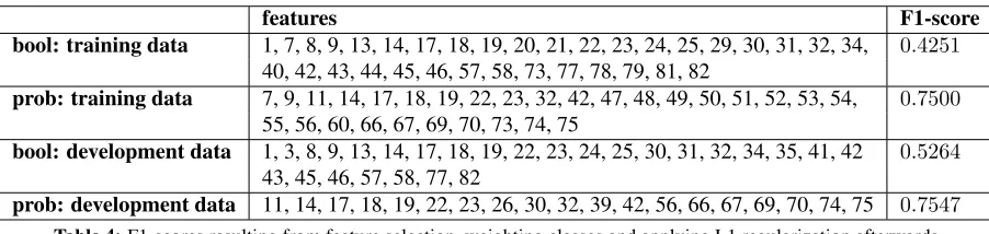
Seeing how setting the right parameters can im-prove the performance of logistic regression, we do another feature selection on the development data. This time we weight the classes as described above and apply L1 regularization from the outset. That way we obtain the feature sets reported in Table 5.
5 Results
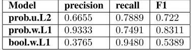
Since the results in Table 5 yield very promising results on the development data, we apply the two models to the test data, which yields comparable re-sults (see modelsbool.w.L1 andprob.w.L1 in Ta-ble 6). Taking a closer look at the individual out-comes, however, reveals that they are by no means expressive. In the binary task our system almost al-ways assignstrue and thereby ensures the high re-call. The precision on the other hand is relatively low and roughly matches the proportion of spurious sentences in the data. Hence our system would be outperformed by one that assignstrueto all samples. Our results on the probabilistic track look similar. Apart from a few instances to which our model as-signs a probability around95%, the estimations are always very close to50%.
In order to examine the effects of a larger set of features we also apply the model resulting from fea-ture selection on the training data to the test data for the probabilistic task. We expect that thanks to the multitude of features this model (prob.u.L2) will eventuate in a more diverse result. Despite the fact that as reported in Table 6 the F1-score drops by 11 points compared to our other system, the indi-vidual outcomes in fact seem to be much more ex-pressive. The results still have a tendency to range around50%but there are considerably more outliers and a lot more probabilities greater than95%.
6 Discussion
6.1 Lessons learned
features F1-score bool: training data 1, 7, 8, 9, 13, 14, 17, 18, 19, 20, 21, 22, 23, 24, 25, 29, 30, 31, 32, 34, 0.4251
40, 42, 43, 44, 45, 46, 57, 58, 73, 77, 78, 79, 81, 82
prob: training data 7, 9, 11, 14, 17, 18, 19, 22, 23, 32, 42, 47, 48, 49, 50, 51, 52, 53, 54, 0.7500 55, 56, 60, 66, 67, 69, 70, 73, 74, 75
bool: development data 1, 3, 8, 9, 13, 14, 17, 18, 19, 22, 23, 24, 25, 30, 31, 32, 34, 35, 41, 42 0.5264 43, 45, 46, 57, 58, 77, 82
[image:8.612.77.528.58.165.2]prob: development data 11, 14, 17, 18, 19, 22, 23, 26, 30, 32, 39, 42, 56, 66, 67, 69, 70, 74, 75 0.7547
Table 4:F1-scores resulting from feature selection, weighting classes and applying L1 regularization afterwards
features F1-score
bool: development data 17, 18, 19, 22, 23, 32, 42, 69, 79 0.5701
prob: development data 17, 18, 19, 22, 23, 32, 42, 44, 72 0.8477
Table 5:F1-scores resulting from feature selection with classes weighted and L1 regularization applied from the outset
weighting the classes beforehand. By weighting the classes inversely proportional to their proportions in the training data, the system is immediately bi-ased towards high probabilities fortruelabels, trying to compensate the superior number of false labels in the training data. Starting the feature selection process with high-precision features, the probabil-ity spikes whenever these features are1. So both the model for the boolean track and the one for the prob-abilistic track start out with very high precisions. Due to the strong true-bias, all other probabilities are close to but still smaller than50%, yielding a rel-atively high recall in the probabilistic system, which results in a very good performance according to the provided evaluation metric. The boolean system, on the other hand, has a very low recall, so in order to increase its F1-score, the precision is sacrificed dur-ing feature selection in favor of a better recall.
The feature selection processes show which fea-tures are more useful than others. We see that most of the integer-valued features that are valuable for readability assessment are never chosen for any model. A possible reason is that readability ease in scientific writing is not as important as in other do-mains, since the target readers are highly educated. A high linguistic complexity is rather characteristic for scientific writing and is possibly not perceived as a deficiency as much.
Interestingly the WordNet features (10, 28) do not work well, in contrast to the features using the pyenchant-package (11, 26).
The number of abbreviations in a paragraph (14) is chosen by every model so it is possible that an
author’s writing style throughout the rest of a doc-ument affects the editor’s acceptance of individual sentences. It is worth considering to design more features that account for consistency in a paragraph. Binary features often manage to improve the models, except for features 15 and 16, which is not surprising, given the fact that they denote exactly op-posite properties and the model is not able to account for dependencies between features. Features 36–39 try to detect number disagreements and seem to per-form poorly. Being based on both dependency trees and part-of-speech tags, these features rely on the correctness of the supplementary data, which in this case has been generated automatically, and hence cannot be guaranteed to be correct.
Our results also show that the domain-related fea-tures are not very helpful in combination with logis-tic regression. We can report that they only make a minor difference in the one model they entered.
Especially the models for probabilistic estimation are improved by features 66, 67 and 69, which are supposed to detect the most unlikely n-grams in a sentence. They are better in detecting local discrep-ancies in a sentence than the maximum likelihood estimation features 59–65, because an unlikely n-gram does not have much impact on the likelihood estimation of a sentence, so even a major error re-flected in a very low n-gram probability can possi-bly go unnoticed. That cannot happen in the features 66–72.
some of the models, which is why we are confident that language modeling is the key to other helpful features yet to be found.
6.2 Evaluation Metric
The evaluation score works well for a system whose only purpose is the identification of erroneous sen-tences, so for the binary classification task the F1-score is perfectly suitable. However, it may be worth considering whether the information that a sentence is fine could be valuable, too. That might be the case whenever sentences must be further processed. In that case the accuracy metric might be the bet-ter choice, because it takes all correct classifications into account, whereas the F1-score does not reward instances correctly classified asfalse.
As for the probabilistic task, our results show that the evaluation score is not strict enough, and that it is prone to misjudge the expressiveness of the re-sults. In fact, correctly assigning 1.0 to only one faulty sentence and0.5to all other sentences yields a score of0.8571. The result is not as extreme if pre-cision and recall are computed based on the mean absolute error, which results in0.6667. This, still, clearly overestimates the quality of the results.
7 Related Work
As Daudaraviˇcius (2015) states, a lot of scientists authoring scientific papers are nonnative English speakers. This insight suggests a relation of auto-matic evaluation of scientific writing to the field of language learner systems. Gamon (2010) mainly ad-dresses article and preposition errors, which have shown to be frequent errors in the dataset provided for the AESW 2016 Shared Task, too. He uses lan-guage models on both a lexical and a syntactical level to find more likely alternatives for prepositions and articles with respect to the linguistic environ-ment they occur in. He also bases some features on ratios of language model outcomes, rather than on individual probabilities, which is an approach that underlies many of our real-valued features.
Tetreault et al. (2010) examine how helpful parser output features are when modeling preposition us-age. They present several phrase structure and dependency-based features, including left and right contexts of constituents in parse trees and the
lexicals modified by a prepositional phrase.
For our features we extract those ideas from these works that seem the most promising for the chal-lenge we encounter. But they both hold inspiration for even more features than those we implement in the course of our participation in the shared task and will be reconsidered in future work.
8 Conclusions
To detect spurious sentences in scientific writing we trained a logistic regression model. After a thor-ough data analysis, which gave us some profound insight into the types of errors occurring in scien-tific writing, we designed a number of features to detect these errors. We identified the most mean-ingful features by performing an incremental feature selection. Some of the resulting features show that corrections which seemed arbitrary might be justi-fied by means of consistency of a text. We also used the probabilities of sentences according to lan-guage models as features, which our feature selec-tion process determined to be helpful. Using the selected features our regression model achieved re-spectable results compared to our competitors’ sys-tems. Weighting our classes during the feature se-lection procedure, we accomplished a score to rank highest according to the evaluation metric in the probabilistic track of the task. However, we dis-covered that these results are very homogeneous and thus not expressive enough for a real life system. For future improvements of our system, we plan on de-veloping an evaluation metric that takes the diversity of result data into account.
Acknowledgements
References
Vidas Daudaraviˇcius. 2015. Automated evaluation of scientific writing: AESW shared task proposal. In
Proceedings of the Tenth Workshop on Innovative Use of NLP for Building Educational Applications, Den-ver, Col., 4 June 2015, pages 56–63.
Michael Gamon. 2010. Using mostly native data to correct errors in learners’ writing: A meta-classifier approach. InProceedings of Human Language Tech-nologies 2010: The Conference of the North American Chapter of the Association for Computational Linguis-tics, Los Angeles, Cal., 2–4 June 2010, pages 163– 171.
Daniel Jurafsky and James H. Martin. 2009. Speech and Language Processing. Pearson Education, Upper Sad-dle River, N.J., second edition.
Emily Pitler and Ani Nenkova. 2008. Revisiting readability: A unified framework for predicting text quality,. In Proceedings of the 2008 Conference on Empirical Methods in Natural Language Process-ing,Waikiki, Honolulu, Hawaii, 25–27 October 2008, pages 186–195.