Optimizing Multivariate Performance Measures
for Learning Relation Extraction Models
Gholamreza Haffari 2Faculty of IT, Monash University [email protected]
Ajay Nagesh1,2,3 1IITB-Monash Research Academy [email protected]
Ganesh Ramakrishnan 3Dept. of CSE, IIT Bombay [email protected]
Abstract
We describe a novel max-margin learn-ing approach to optimize non-linear perfor-mance measures for distantly-supervised re-lation extraction models. Our approach can be generally used to learn latent variable models under multivariate non-linear perfor-mance measures, such as Fβ-score. Our approach interleaves Concave-Convex Pro-cedure (CCCP) for populating latent vari-ables with dual decomposition to factorize the original hard problem into smaller inde-pendent sub-problems. The experimental re-sults demonstrate that our learning algorithm is more effective than the ones commonly used in the literature for distant supervision of in-formation extraction models. On several data conditions, we show that our method outper-forms the baseline and results in up to 8.5% improvement in theF1-score.
1 Introduction
Rich models with latent variables are popular for many problems in natural language processing. In information extraction, for example, one needs to predict the relation labelsythat an entity-pairxcan have based on the hidden relation mentionsh,i.e., the relation labels for occurrences of the entity-pair in a given corpus. However, these models are often trained by optimizing performance measures (such as conditional log-likelihood or error rate) that are not directly related to the task-specific non-linear performance measure,e.g., the F1-score. However,
better models may be trained by optimizing the task-specific performance measure while allowing latent variables to adapt their values accordingly.
We present a large-margin method to learn pa-rameters of latent variable models for a wide range of non-linear multivariate performance mea-sures such as Fβ. Our method can be applied
to learning graphical models that incorporate inter-dependencies among the output variables either di-rectly, or indirectly through hidden variables.
Large-margin methods have been shown to be a compelling approach to learn rich models detailing the inter-dependencies among the output variables, via optimizing loss functions decomposable over the
training instances (Taskar et al., 2003; Tsochan-taridis et al., 2004) or non-decompasable loss func-tions (Ranjbar et al., 2013; Tarlow and Zemel, 2012; Rosenfeld et al., 2014; Keshet, 2014). They have also been shown to be powerful when applied to la-tent variable models when optimizing for decompos-able loss functions (Wang and Mori, 2011; Felzen-szwalb et al., 2010; Yu and Joachims, 2009).
Our large-margin method learns latent variable models via optimizing non-decomposable loss func-tions. It interleaves the Concave-Convex Procedure (CCCP) (Yuille and Rangarajan, 2001) for populat-ing latent variables with dual decomposition (Ko-modakis et al., 2011; Rush and Collins, 2012). The latter factorizes the hard optimization problem (encountered in learning) into smaller independent sub-problems over the training instances. We then present linear programming and local search meth-ods for effective optimization of the sub-problems encountered in the dual decomposition. Our local search algorithm leads to a speed up of 7,000 times compared to the exhaustive search used in the liter-ature (Joachims, 2005; Ranjbar et al., 2012).
Our work is the first to make use of max-margin training in distant supervision of relation extraction models. We demonstrate the effectiveness of our proposed method compared to two strong baseline systems which optimize for the error rate and con-ditional likelihood, including a state-of-the-art sys-tem by Hoffmann et al. (2011). On several data con-ditions, we show that our method outperforms the baseline and results in up to 8.5% improvement in theF1-score.
Figure 1: Graphical model instantiated for entity pairx:= Barack Obama, United States
2 Preliminaries
2.1 Distant Supervision for Relation Extraction
Our framework is motivated by distant supervision for learning relation extraction models (Mintz et al., 2009). The goal is to learn relation extraction mod-els by aligning facts in a database to sentences in a large unlabeled corpus. Since the individual sen-tences are not hand labeled, the facts in the database act as “weak” or “distant” labels, hence the learning scenario is termed as distantly supervised.
Prior work casts this problem as a multi-instance multi-label learning problem (Hoffmann et al., 2011; Surdeanu et al., 2012). It is multi-instance since for a given entity-pair, only the label of the bag of sentences containing both entities (aka mentions) is given. It is multi-label since a bag of mentions can have multiple labels. The inter-dependencies between relation labels and (hidden) mention labels are modeled by a Markov Random Field (Figure 1) (Hoffmann et al., 2011). The learning algorithms used in the literature for this problem optimize the (conditional) likelihood, but the evaluation measure is commonly theF-score.
Formally, the training data isD := {(xi,yi)}Ni=1
wherexi ∈ X is the entity-pair, yi ∈ Y denotes
the relation labels, andhi ∈ H denotes the
hid-denmention labels. The possible relation labels for the entity pair are observed from a given knowledge-base. If there areLcandidate relation labels in the knowledge-base, thenyi ∈ {0,1}L, (e.g.yi,`is 1 if
the relation`is licensed by the knowledge-base for the entity-pair) andhi ∈ {1, .., L,nil}|xi|(i.e. each
mention realizes one of the relation labels ornil).
Notation. In the rest of the paper, we denote the collection of all entity-pairs{xi}Ni=1byX ∈X := X × .. × X, the collection of mention relations
{hi}Ni=1byH∈H:=H×..×H, and the collection
of relation labels{yi}Ni=1byY∈Y :=Y ×..× Y.
The aim is to learn a parameter vectorw∈Rdby
which the relation labels for a new entity-pairxcan be predicted
fw(x) := arg maxy max
h w·Φ(x,h,y) (1)
whereΦ∈Rdis a feature vector defined according
to the Markov Random Field, modeling the inter-dependencies betweenxandythroughh(Figure 1). In training, we would like to minimize the loss func-tion ∆by which the model will be assessed at test time. For the relation extraction task, the loss can be considered to be the negative of theFβ score:
Fβ = β 1
Precision +Recall1−β
(2)
where β = 0.5 results in optimizing against F1
-score. Our proposed learning method optimizes those loss functions∆which cannot be decomposed over individual training instances. For example,Fβ
depends non-linearly on Precision and Recall which in turn require the predictions forallthe entity pairs in the training set, hence it cannot be decomposed over individual training instances.
2.2 Structured Prediction Learning
The goal of our learning problem is to findw∈Rd
new sampleD0 of sizeN0:
R∆
fw:=
Z
∆ fw(x01), .., fw(x0N0), y01, ..,y0N0
dP r(D0)
(3)
Generally, the loss function ∆cannot be decom-posed into a linear combination of a loss function δ over individual training samples. However, most discriminative large-margin learning algorithms as-sume for simplicity that the loss function is decom-posable and the samples are i.i.d. (independent and identically distributed), which simplifies the sample riskR∆
fw as:
Rδfw :=
Z
δ(fw(x0),y0)dP r(x0,y0) (4)
Often learning algorithms make use of the empirical risk as an approximation of the sample risk:
ˆ
Rδfw := N1
N X
i=1
δ(fw(xi),yi) (5)
For non-decomposable loss functions, such as Fβ,
∆cannot be expressed in terms of instance-specific loss functionδto construct the empirical risk of the kind in Eq. (5). Instead, we need to optimize the empirical risk constructed based on the sample loss:
ˆ
R∆ fw := ∆
fw(x1), .., fw(xN), y1, ..,yN
(6) or equivalently
ˆ
Rf∆w := ∆(fw(X),Y) (7)
wherefw(X) := (fw(x1), .., fw(xN)).
Having defined the empirical risk in Eq (7), we formulate the learning problem as a structured pre-diction problem. Instead of learning a mapping functionfw : X → Y from an individual instance x ∈ X to its label y ∈ Y, let us learn a mapping functionf : X → Y from all instancesX ∈ X to their labelsY∈Y. We then define the best labeling using a linear discriminant function:
f(X) := arg max
Y0∈YHmax∈H
n
w·Ψ(X,H,Y0)o (8)
whereΨ(X,H,Y0) := PN
i=1Φ(xi,hi,y0i). Based
on the margin re-scaling formulation of structured prediction problems (Tsochantaridis et al., 2004),
the training objective can be written as the follow-ing unconstrained optimization problem:
min
w
1
2||w||22+CmaxY0
n
max
H w·Ψ(X,H,Y 0)
−max
H w·Ψ(X,H,Y) + ∆(Y
0,Y)o (9)
which is similar to the training objective for the la-tent SVMs (Yu and Joachims, 2009), with the differ-ence that instance-dependent loss function δ is re-placed by the sample loss function∆. Learningw
by optimizing the above objective function is chal-lenging, and is the subject of the next section.
3 Optimizing the Training Objective
In this section we present our method to learn latent SVMs with non-decomposable loss functions. Our training objective is Eq (9), which can be equiva-lently expressed as:
minw 1
2||w||22+Cy0max
1,..,y0N
∆
(y1, ..,yN),(y01, ..,y0N)
+XN i=1
max
h w·Φ(xi,h,y 0 i)−
N X
i=1
max
h w·Φ(xi,h,yi)
(10)
The training objective is non-convex, since it is the difference of two convex functions. In this section we make use of the CCCP to populate the hidden variables (Yu and Joachims, 2009; Yuille and Ran-garajan, 2001), and interleave it with dual decompo-sition (DD) to solve the resulting intermediate loss-augmented inference problems (Ranjbar et al., 2012; Rush and Collins, 2012; Komodakis et al., 2011).
3.1 Concave-Convex Procedure (CCCP)
The CCCP (Yuille and Rangarajan, 2001) gives a general iterative method to optimize those non-convex objective functions which can be written as the difference of two convex functions g1(w) −
g2(w). The idea is to iteratively lowerboundg2with
a linear functiong2(w(t)) +v·(w−w(t)), and take
the following step to updatew:
w(t+1) := arg min
w
g1(w)−w·v(t) (11)
Algorithm 1The Training Algorithm (Optimizing Eq 10) 1: procedureOPT-LATENTSVM(X,Y)
2: Initializew(0)and sett= 0 3: repeat
4: fori:= 1 to Ndo
5: h∗
i := arg maxhw(t)·Φ(xi,h,yi)
// Optimizing Eq 12
6: w(t+1):=optSVM(X,H∗,Y) 7: t:=t+ 1
8: untilsome stopping condition is met 9: returnw(t)
lowerbound of g2(w) involves populating the
hid-den variables by:
h∗i := arg max
h
w(t)·Φ(xi,h,yi) .
Therefore, in each iteration of our CCCP-based al-gorithm we need to optimize Eq (12), which is rem-iniscent of the standard structural SVM without la-tent variables:
min w
1
2||w||22+Cy0max
1,..,y0N
∆
(y1, ..,yN),(y01, ..,y0N)
+ N X i=1 max
h w·Φ(xi,h,y 0 i)−
N
X
i=1
w·Φ(xi,h∗i,yi)
(12)
The above objective function can be optimized us-ing the standard cuttus-ing-plane algorithms for struc-tural SVM (Tsochantaridis et al., 2004; Joachims, 2005). The cutting-plane algorithm in turn needs to solve theloss-augmented inference, which is the subject of the next sub-section. The CCCP-based training algorithm is summarized in Algorithm 1.
3.2 Loss-Augmented Inference
To be able to optimize the training objective Eq (12) encountered in each iteration of Algorithm 1, we need to solve (the so-called) loss-augmented infer-ence:
max
y0
1,..,y0N ∆
(y1, ..,yN),(y10, ..,y0N)
+XN i=1
max
h w·Φ(xi,h,y 0
i) (13)
We make use of the dual decomposition (DD) tech-nique to decouple the two terms of the above ob-jective function, and efficiently find an approximate solution. DD is shown to be an effective technique for loss-augmented inference in structured predic-tion modelswithouthidden variables (Ranjbar et al., 2012).
To apply DD to the loss-augmented inference (13), let us rewrite it as a constrained optimization problem:
max
y0
1,...,y0N,y001,...,y00N ∆
(y1, . . . ,yN),(y01, . . . ,y0N)
+XN i=1
max
h w·Φ(xi,h,yi 00)
subject to
∀i∈ {1, . . . , N},∀`∈ {1, . . . , L}, y0
i,`=y00i,`
Introduction of the new variables (y00
1, ..,yN00)
de-couples the two terms in the objective function, and as we will see, leads to an effective optimization al-gorithm. After forming the Lagrangian, the dual ob-jective function is derived as:
L(Λ) := max
Y0 ∆(Y,Y
0) +X
i X ` λi(`)y0 i,`+ max Y00 N X i=1 max
h w·Φ(xi,h,yi
00)−X
i
X
`
λi(`)yi,`00
whereΛ := (λλλ1, ..,λλλN), andλλλi is a vector of
La-grange multipliers for L binary variables each of which represent a relation label. The two optimiza-tion problems involved in the dual L(Λ) are inde-pendent and can be solved separately. The dual is an upperbound on the loss-augmented objective func-tion for any value of Λ; therefore, we can find the tightest upperbound as an approximate solution:
min
Λ L(Λ)
The dual is non-differentiable at those points Λ
where either of the two optimisation problems has multiple optima. Therefore, it is optimized using the subgradient descent method:
Λ(t):= Λ(t−1)−η(t)(Y0
∗−Y∗00) whereη(t)= √1
tis the step size1, and
Y∗0 := arg max
Y0 ∆(Y,Y
0) +X
i
X
`
λ(ti−1)(`)y0
i,` (14)
Y00∗ := arg max
Y00 N
X
i=1 max
h w·Φ(xi,h,yi 00)
−X
i
X
`
λ(ti−1)(`)y00
i,` (15)
1Other (non-increasing) functions of the iteration numbert
are also plausible, as far as they satisfy the following condi-tions (Komodakis et al., 2011) needed to guarantee the conver-gence to the optimal solution in the subgradient descent method: η(t)≥0,lim
Algorithm 2Loss-Augmented Inference
1: procedureOPT-LOSSAUG(w,X,Y)
2: InitializeΛ(0)and sett= 0 3: repeat
4: Y∗0 :=opt-LossLag(Λ,Y) // Eq (14) 5: Y∗00:=opt-ModelLag(Λ,X) // Eq (15) 6: ifY∗0 =Y00∗ then
7: returnY∗0
8: fori:= 1 to Ndo
9: for`:= 1 to Ldo
10: λ(it+1)(`) :=λi(t)(`)−η(t)(y0
i,`−y00i,`)
11: untilsome stopping condition is met 12: returnY0∗
The DD algorithm to compute the loss-augmented inference is outlined in Algorithm 2. Now the chal-lenge is how to solve the above two optimization problems, which is the subject of the following sec-tion.
3.3 Effective Optimization of the Dual
The two optimization problems involved in the dual are hard in general. More specifically, the optimiza-tion of the affine-augmented model score (in Eq. 15) is as difficult as the MAP inference in the underlying graphical model, which can be challenging for loopy graphs. For the graphical model underlying distant supervision of relation extraction (Fig 1), we formu-late the inference as an ILP (integer linear program). Furthermore, we relax the ILP to LP to speed up the inference, in the expense of trading exact solutions with approximate solutions2.
Likewise, the optimization of the affine-augmented multivariate loss (in Eq. 14) is difficult. This is because we have to search over the entire space of Y0 ∈ Y, which is exponentially large
O(2N∗L). However, if the loss term ∆ can be
expressed in terms of some aggregate statistics over Y0, such as false positives (FPs) and false negatives (FNs), the optimization can be performed efficiently. This is due to the fact that the number of FPs can range from zero to the size of negative labels, and the number of FNs can range from zero to the number of positive labels. Therefore, the loss term can takeO(N2L2) different values which can
2We observed in our experiments that relaxing the ILP to
LP does not hurt the performance, but significantly speeds up the inference.
Algorithm 3FindingY0
∗: Local Search
1: procedureOPT-LOSSLAG(Λ,Y)
2: (idxn
1. . . idxn#neg)←Sort↓(λi(`))// FPs 3: (idxn
1. . . idxn#pos)←Sort↑(λi(`))// FNs 4: Initialise(fp, fn)on the grid
5: repeat
6: for((fp0, fn0)∈Neigbours(fp, fn)do 7: loss(fp0,fn0)=∆(fp0, fn0) +Λsorted3 8: loss(fp00,fn00)=arg max(fp0,fn0)loss(fp0,fn0) 9: ifloss(fp,fn)> loss(fp00,fn00)then
10: break
11: else
12: (fp, fn) = (fp00, fn00) 13: untilloss(fp,fn)≤loss(fp00,fn00) 14: return{Y0corresponding to(fp, fn)}
be represented on a two-dimensional grid. Fixing FPs and FNs to a grid point, Λ·Y0 is maximized with respect to Y0. The grid point which has the best value for∆(Y,Y0) +Λ·Y0will then give the optimal solution for Eq (14).
Exhaustive search in the space of all possible grid points is not efficient as soon as the grid becomes large. Therefore, we have to adapt the techniques proposed in previous work (Ranjbar et al., 2012; Joachims, 2005). We propose a simple but effective
local searchstrategy for this purpose. The procedure is outlined in Algorithm 3. We start with a random grid point, and move to the best neighbour. We keep hill climbing until there is no neighbour better than the current point. We define the neighbourhood by a set of exponentially-spaced points in all directions around the current point, to improve the exploration of the search space. We present some analysis on the benefits of using this search strategy vis-a-vis the ex-haustive search in the Experiments section.
4 Experiments
Dataset:We use the challenging benchmark dataset created by Riedel et al. (2010) for distant supervi-sion of relation extraction models. It is created by aligning relations fromFreebase4with the sentences in New York Times corpus (Sandhaus, 2008). The labels for the datapoints come from the Freebase 3For a given(fp, fn), we sety0by picking the sorted unary
terms that maximize the score according toy.
database but Freebase is incomplete (Ritter et al., 2013). So a data point is labelednilwhen either no relation exists or the relation is absent in Freebase. To avoid this ambiguity we train and evaluate the baseline and our algorithms on a subset of this dataset which consists of only non-nil relation labeled datapoints (termed as positive dataset). For the sake of completeness, we do report the accuracies of the various approaches on the entire evaluation dataset.
Systems and Baseline: Hoffmann et al. (2011) describe a state-of-the-art approach for this task. They use a perceptron-style parameter update scheme adapted to handle latent variables; their training objective is the conditional likelihood. Out of the two implementations of this algorithm, we use the better5 of these two6, as our baseline (denoted by Hoffmann). For a fair comparison, the training dataset and the set of features defined over it are common to all the experiments.
We discuss the results of two of our approaches. One, is the LatentSVM max-margin formulation with the simple decomposable Hamming loss function which minimizes the error rate (denoted by
MM-hamming). The other is the LatentSVM max-margin formulation with the non-decomposable loss function which minimizes the negative of Fβ score
(denoted byMM-F-loss)7.
Evaluation Measure: The performance mea-sure isFβ which can be expressed in terms of false
positives (FP) and false negatives (FN) as:
Fβ=β(F PNp−−F N) +F N N p
where β is the weight assigned to precision (and 1−βto recall).F P,F N andNpare defined as :
F P = X i
X
` y0
i,`(1−yi,l)
F N = X i
X
`
yi,`(1−y0
i,l)
Np = X i
X
` yi,`
5It is not quite clear why the performance of the two
imple-mentations are different.
6nlp.stanford.edu/software/mimlre.shtml 7We use a combination of F1 loss and hamming loss, as
[image:6.612.314.567.55.213.2]us-ing only F1-loss overfits the trainus-ing dataset, as observed from the experiments.
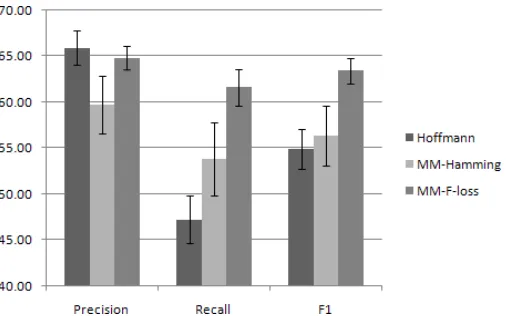
Figure 2: Experiments on 10% Riedel datasets.
Precision Recall F1
Hoffmann 65.93 47.22 54.91
MM-Hamming 59.74 53.81 56.32
MM-F-loss 64.81 61.63 63.44
Table 1: Average results on 10% Riedel datasets.
We use1−Fβas the expression for the
multivariate-loss.
4.1 Training on Sub-samples of Data
We performed a number of experiments using differ-ent randomized subsets of the Riedel dataset (10% of the positive dataset) for training the max-margin approaches. This was done in order to empirically determine a good set of parameters for training. We also compare the results of the approaches with
Hoffmanntrained on the same sub-samples.
[image:6.612.87.254.554.636.2]Comparison with the Baseline:We report the aver-age over 15 subsets of the dataset with a 90% confi-dence interval (using student-t distribution). The re-sults of these experiments are shown in Figure 2 and Table 1. We observe that bothMM-hamming and
MM-F-losshave higherF1-score compared to the
baseline. There is a significant improvement inF1
-score to the tune of 8.52% for the multivariate per-formance measure overHoffmann. There is also an improvement ofF1-score of 7.12% compared to MM-Hamming. This highlights the importance of using non-linear loss functions compared to simple loss functions like error rate during training.
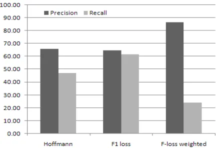
Figure 3: Weighting of Precision and Recall (β= 0.833)
due to over-fitting the data, as the performance on the training datasets were very high. One more interesting observation of MM-F-loss is that it is fairly balanced w.r.t both precision and recall which the other approaches do not exhibit.
Tuning towards Precision/Recall: Often we come across situations where either precision or recall is important for a given application. This is modeled by the notion of Fβ (van Rijsbergen,
1979). One of the main advantages of using a non-decomposable loss function like Fβ is the
ability to vary the learning algorithm to factor such situations. For instance we can tune the objective to favor precision more than recall by “up-weighting” precision in theFβ-score.
For instance, in the previous case we observed thatMM-F-losshas a marginally poorer precision
compared to Hoffmann. Suppose we increase
the weight of precision, β = 0.833, we observe a dramatic increase in precision from 65.83% to 86.59%. As expected, due to the precision-recall trade-off, we observe a decrease in recall. The results are shown in Figure 3.
Local vs. Exhaustive Grid Search: As we described in Section 3.3, we devise a simple yet efficient local search strategy to search the space of (F P, F N) grid-points. This enables a speed up of three orders of magnitude in solving the dual-optimization problem. In Table 2, we compare the average time per iteration and the F1-score
[image:7.612.312.566.55.207.2]when each of these techniques is used for training on a sub-sample dataset. We observe that there
Figure 4: Overall accuracies Riedel dataset
avg. time per iter. F1
Local Search 0.09s 58.322
Exhaustive Search 630s 58.395
Table 2: Local vs. Exhaustive Search.
is a significant decrease in training time when we use local search (almost 7000 times faster), with a negligible decrease inF1-score (0.073%).
4.2 The Overall Results
Figure 4 and Table 3 present the overall results of our approaches compared to the baseline on the pos-itivedataset. We observe that MM-F-losshas an increase inF1-score to the tune of ∼8% compared
to the baseline. This confirms our observation on the sub-sample datasets we saw earlier.
By assigning more weight to precision, we are able to improve over the precision of Hoffmann
by∼1.6% (Table 4). When precision is tuned with a higher weight during training ofMM-F-loss, we see an improvement in precision without much dip in recall.
Precision Recall F1
Hoffmann 75.436 46.615 57.623
MM-Hamming 76.839 50.462 60.918
[image:7.612.316.530.627.687.2]MM-F-loss 65.991 65.211 65.598
Precision Recall Fβ
Hoffmann 75.44 46.62 57.62
[image:8.612.74.280.57.102.2]MM-F-loss-wt 77.04 53.44 63.11
Table 4: Increasing weight on Precision inFβ.
4.3 Discussion
So far we have discussed the performance of var-ious approaches on the positiveevaluation dataset. Our approach is shown to improve overallFβ-score
having better recall than the baseline. By suitably tweaking theFβ we show an improvement in
preci-sion as well.
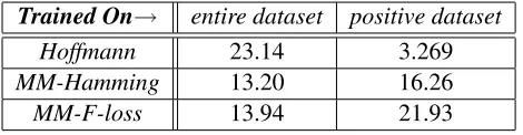
The performance of the approaches when evalu-ated on the entire test dataset (consisting of both nil and non-nil datapoints) is shown in Table 5. Max-margin based approaches generally perform well when trained only on thepositivedataset compared to Hoffmann. However, our F1-scores are ∼8%
less when we train on the entire dataset consisting of both nil and non-nil datapoints.
Trained On→ entire dataset positive dataset
Hoffmann 23.14 3.269
MM-Hamming 13.20 16.26
MM-F-loss 13.94 21.93
Table 5:F1-scores on the entire test set.
In a recent work, Xu et al. (2013) provide some statistics about the incompleteness of the Riedel dataset. Out of the sampled 1854 sentences from NYTimes corpus most of the entity pairs expressing a relation in Freebase correspond to false negatives. This is one of the reasons why we do not consider nil labeled datapoints during training and evaluation.
MIMLRE (Surdeanu et al., 2012) is another state-of-the-art system which is based on the EM algo-rithm. Since that system uses an additional set of features for the relation variablesy, it is not our pri-mary baseline. On the positive dataset, our model
MM-F-lossachieves aF1-score of 65.598%
com-pared to 65.341% of MIMLRE. As part of the future work, we would like to incorporate the additional features present in MIMLRE into our approach.
5 Conclusion
In this paper, we described a novel max-margin approach to optimize non-linear performance mea-sures, such as Fβ, in distant supervision of
infor-mation extraction models. Our approach is general and can be applied to other latent variable models in NLP. Our approach involves solving the hard-optimization problem in learning by interleaving Concave-Convex Procedure with dual decomposi-tion. Dual decomposition allowed us to solve the hard sub-problems independently. A key aspect of our approach involves a local-search algorithm which has led to a speed up of 7,000 times in our ex-periments. We have demonstrated the efficacy of our approach in distant supervision of relation extrac-tion. Under several conditions, we have shown our technique outperforms very strong baselines, and re-sults in up to 8.5% improvement inF1-score.
For future work, we would like to maximize other performance measures, such as area under the curve, for information extraction models. Furthermore, we would like to explore our approach for other latent variable models in NLP, such as those in machine translation.
Acknowledgements
Gholamreza Haffari is grateful to National ICT Aus-tralia (NICTA) for their generous funding, as part of the Machine Learning Collaborative Research Projects. Ajay Nagesh acknowledges Xerox Re-search Centre India (XRCI) for their travel support in the form of International Student Travel grant.
References
Pedro F. Felzenszwalb, Ross B. Girshick, David A. McAllester, and Deva Ramanan. 2010. Object detec-tion with discriminatively trained part-based models.
IEEE Trans. Pattern Anal. Mach. Intell., 32(9):1627– 1645.
[image:8.612.71.306.389.450.2]T. Joachims. 2005. A support vector method for multi-variate performance measures. InInternational Con-ference on Machine Learning (ICML), pages 377–384. Joseph Keshet. 2014. Optimizing the measure of per-formance in structured prediction. In Jeremy Jancsary Sebastian Nowozin, Peter V. Gehler and Christoph H. Lampert, editors, Advanced Structured Prediction. The MIT Press.
Nikos Komodakis, Nikos Paragios, and Georgios Tziri-tas. 2011. Mrf energy minimization and beyond via dual decomposition. IEEE Transactions on Pattern Analysis and Machine Intelligence, 33(3):531–552. Mike Mintz, Steven Bills, Rion Snow, and Dan Jurafsky.
2009. Distant supervision for relation extraction with-out labeled data. InProceedings of the Joint Confer-ence of the 47th Annual Meeting of the ACL and the 4th International Joint Conference on Natural Language Processing of the AFNLP: Volume 2 - Volume 2, ACL ’09, pages 1003–1011, Stroudsburg, PA, USA. Asso-ciation for Computational Linguistics.
Mani Ranjbar, Arash Vahdat, and Greg Mori. 2012. Complex loss optimization via dual decomposition. In
2012 IEEE Conference on Computer Vision and Pat-tern Recognition, Providence, RI, USA, June 16-21, 2012, pages 2304–2311.
Mani Ranjbar, Tian Lan, Yang Wang, Stephen N. Robi-novitch, Ze-Nian Li, and Greg Mori. 2013. Opti-mizing nondecomposable loss functions in structured prediction. IEEE Trans. Pattern Anal. Mach. Intell., 35(4):911–924.
Sebastian Riedel, Limin Yao, and Andrew McCallum. 2010. Modeling relations and their mentions with-out labeled text. InProceedings of the 2010 European conference on Machine learning and knowledge dis-covery in databases: Part III, ECML PKDD’10, pages 148–163, Berlin, Heidelberg. Springer-Verlag. Alan Ritter, Luke Zettlemoyer, Mausam, and Oren
Et-zioni. 2013. Modeling missing data in distant super-vision for information extraction. TACL, 1:367–378. Nir Rosenfeld, Ofer Meshi, Amir Globerson, and Daniel
Tarlow. 2014. Learning structured models with the auc loss and its generalizations. In Proceedings of the 17th International Conference on Artificial Intel-ligence and Statistics (AISTATS).
Alexander M. Rush and Michael Collins. 2012. A tuto-rial on dual decomposition and lagrangian relaxation for inference in natural language processing. J. Artif. Intell. Res. (JAIR), 45:305–362.
E. Sandhaus. 2008. The new york times annotated cor-pus.
Mihai Surdeanu, Julie Tibshirani, Ramesh Nallapati, and Christopher D. Manning. 2012. Multi-instance multi-label learning for relation extraction. In
Proceed-ings of the 2012 Joint Conference on Empirical Meth-ods in Natural Language Processing and Computa-tional Natural Language Learning, EMNLP-CoNLL ’12, pages 455–465, Stroudsburg, PA, USA. Associa-tion for ComputaAssocia-tional Linguistics.
Daniel Tarlow and Richard S Zemel. 2012. Structured output learning with high order loss functions. In Pro-ceedings of the 15th Conference on Artificial Intelli-gence and Statistics.
Benjamin Taskar, Carlos Guestrin, and Daphne Koller. 2003. Max-margin markov networks. InNIPS. I. Tsochantaridis, T. Hofmann, T. Joachims, and Y. Altun.
2004. Support vector machine learning for interde-pendent and structured output spaces. InInternational Conference on Machine Learning (ICML), pages 104– 112.
C. J. van Rijsbergen. 1979. Information retrieval. But-terworths, London, 2 edition.
Yang Wang and Greg Mori. 2011. Hidden part mod-els for human action recognition: Probabilistic versus max margin. IEEE Trans. Pattern Anal. Mach. Intell., 33(7):1310–1323.
Wei Xu, Raphael Hoffmann, Le Zhao, and Ralph Gr-ishman. 2013. Filling knowledge base gaps for dis-tant supervision of relation extraction. In Proceed-ings of the 51st Annual Meeting of the Association for Computational Linguistics (Volume 2: Short Papers), pages 665–670, Sofia, Bulgaria, August. Association for Computational Linguistics.
Chun-Nam John Yu and Thorsten Joachims. 2009. Learning structural svms with latent variables. In Pro-ceedings of the 26th Annual International Conference on Machine Learning, ICML 2009, Montreal, Quebec, Canada, June 14-18, 2009, page 147.