Multiview LSA: Representation Learning via Generalized CCA
Pushpendre Rastogi1 and Benjamin Van Durme1,2 and Raman Arora1 1Center for Language and Speech Processing
2Human Language Technology Center of Excellence Johns Hopkins University
Abstract
Multiview LSA (MVLSA) is a generalization of Latent Semantic Analysis (LSA) that sup-ports the fusion of arbitrary views of data and relies on Generalized Canonical Correlation Analysis (GCCA). We present an algorithm for fast approximate computation of GCCA, which when coupled with methods for han-dling missing values, is general enough to ap-proximate some recent algorithms for induc-ing vector representations of words. Exper-iments across a comprehensive collection of test-sets show our approach to be competitive with the state of the art.
1 Introduction
Winograd (1972) wrote that: “Two sentences are
paraphrases if they produce the same representation in the internal formalism for meaning”. This intu-ition is made soft in vector-space models (Turney and Pantel, 2010), where we say that expressions in language are paraphrases if their representations are
closeunder some distance measure.
One of the earliest linguistic vector space mod-els was Latent Semantic Analysis (LSA). LSA has been successfully used for Information Retrieval but it is limited in its reliance on a single matrix, or
view, of term co-occurrences. Here we address the
single-view limitation of LSA by demonstrating that the framework of Generalized Canonical Correla-tion Analysis (GCCA) can be used to perform Mul-tiview LSA (MVLSA). This approach allows for the use of an arbitrary number of views in the induc-tion process, including embeddings induced using other algorithms. We also present a fast approx-imate method for performing GCCA and
approxi-mately recover the objective of (Pennington et al., 2014) while accounting for missing values.
Our experiments show that MVLSA is com-petitive with state of the art approached for inducing vector representations of words and phrases. As a methodological aside, we discuss the (in-)significance of conclusions being drawn from comparisons done on small sized datasets.
2 Motivation
LSA is an application of Principal Component Anal-ysis (PCA) to a term-document cooccurrence ma-trix. The principal directions found by PCA form the basis of the vector-space in which to represent the input terms (Landauer and Dumais, 1997). A drawback of PCA is that it can leverage only a sin-gle source of data and it is sensitive to scaling.
An arguably better approach to representation learning is Canonical Correlation Analysis (CCA)
that induces representations that are maximally
cor-relatedacross two views, allowing the utilization of two distinct sources of data. While an improvement over PCA, being limited to only two views is un-fortunate in light of the fact that many sources of data (perspectives) are frequently available in prac-tice. In such cases it is natural to extend CCA’s orig-inal objective of maximizing correlation between two views by maximizing some measure of the
ma-trixΦthat contains all the pairwise correlations
be-tween linear projections of the covariates. This
is how Generalized Canonical Correlation Analy-sis (GCCA) was first derived by Horst (1961). Re-cently these intuitive ideas about benefits of lever-aging multiple sources of data have received strong theoretical backing due to the work by Sridharan and
Kakade (2008) who showed that learning with mul-tiple views is beneficial since it reduces the com-plexity of the learning problem by restricting the search space. Recent work by Anandkumar et al. (2014) showed that at least three views are neces-sary for recovering hidden variable models.
Note that there exist different variants of GCCA
depending on the measure of Φthat we choose to
maximize. Kettenring (1971) enumerated a variety of possible measures, such as the spectral-norm of
Φ. Kettenring noted that maximizing this
spectral-norm is equivalent to finding linear projections of the covariates that are most amenable to rank-one PCA, or that can be best explained by a single term
factor model. This variant was named MAX-VAR
GCCAand was shown to be equivalent to a proposal
by Carroll (1968), which searched for an auxiliary
orthogonal representation G that was maximally
correlated to the linear projections of the covariates. Carroll’s objective targets the intuition that represen-tations leveraging multiple views should correlate with all provided views as much as possible.
3 Proposed Method: MVLSA
LetXj ∈RN×dj ∀j ∈ [1, . . . , J]be the mean
cen-tered matrix containing data from viewj such that
row iofXj contains the information for wordwi.
Let the number of words in the vocabulary beN and
number of contexts (columns inXj) bedj.
Follow-ing standard notation (Hastie et al., 2009) we call
X>
j Xj the scatter matrix andXj(Xj>Xj)−1Xj>the
projection matrix.
The objective ofMAX-VAR GCCAcan be written
as the following optimization problem: Find G ∈
RN×randU
j ∈Rdj×rthat solve:
arg min G,Uj
J X
j=1
G−XjUj2 F
subject toG>G=I.
(1)
The matrix Gthat solves problem (1) is our vector
representation of the vocabulary. FindingGreduces
to spectral decomposition of sum of projection
ma-trices of different views: Define
Pj =Xj(Xj>Xj)−1Xj>, (2)
M =XJ j=1
Pj. (3)
Then, for some positive diagonal matrixΛ, Gand
Uj satisfy:
MG=GΛ, (4)
Uj =
Xj>Xj −1
Xj>G. (5)
Computationally storing Pj ∈ RN×N is
prob-lematic owing to memory constraints. Further, the scatter matrices may be non-singular leading to an ill-posed procedure. We now describe a novel
scal-able GCCA with`2-regularization to address these
issues.
Approximate Regularized GCCA: GCCA can be regularized by addingrjI to scatter matrixXj>Xj
before doing the inversion whererj is a small
con-stant e.g. 10−8. Projection matrices in (2) and (3)
can then be written as
e
Pj =Xj(Xj>Xj+rjI)−1Xj>, (6)
M =XJ j=1
e
Pj. (7)
Next, to scale up GCCA to large datasets, we
first form a rank-mapproximation of projection
ma-trices (Arora and Livescu, 2012) and then extend
it to an eigendecomposition forM following ideas
by Savostyanov (2014). Consider the rank-mSVD
ofXj:
Xj =AjSjBj>,
whereSj ∈ Rm×m is the diagonal matrix withm
-largest singular values ofXj andAj ∈ RN×m and
Bj ∈ Rm×dj are the corresponding left and right
singular vectors. Given this SVD, write thejth
pro-jection matrix as
e
Pj = AjSj>(rjI+SjSJ>)−1SjA>j, = AjTjTj>A>j,
where Tj ∈ Rm×m is a diagonal matrix such that
that the sum of projection matrices can be expressed asM = ˜MM˜>where
˜
M = [A1T1. . . AJTJ]∈RN×mJ.
Therefore, eigenvectors of matrix M, i.e. the
ma-trixGthat we are interested in finding, are the left
singular vectors of M˜, i.e. M˜ = GSV>. These
left singular vectors can be computed by using
In-cremental PCA (Brand, 2002) sinceM˜ may be too
large to fit in memory.
3.1 Computing SVD of mean centeredXj
Recall that we assumedXj to be mean centered
ma-trices. Let Zj ∈ RN×dj be sparse matrices
con-taining mean-uncentered cooccurrence counts. Let
fj = nj ◦tj be the preprocessing function that we
apply toZj:
Yj =fj(Zj), (8) Xj =Yj−1(1>Yj). (9)
In order to compute the SVD of mean centered
ma-trices Xj we first compute the partial SVD of
un-centered matrixYjand then update it (Brand (2006)
provides details). We experimented with
represen-tations created from the uncentered matricesYj and
found that they performed as well as the mean cen-tered versions but we would not mention them fur-ther since it is computationally efficient to follow the principled approach. We note, however, that even the method of mean-centering the SVD produces an approximation.
3.2 Handling missing rows across views
With real data it may happen that a term was not observed in a view at all. A large number of missing rows can corrupt the learnt representations since the rows in the left singular matrix become zero. To counter this problem we adopt a variant of the “missing-data passive” algorithm from Van De Velden and Bijmolt (2006) who modified the GCCA objective to counter the problem of missing
rows.1 The objective now becomes:
arg min G,Uj
J X
j=1
Kj(G−XjUj)2 F
subject toG>G=I,
(10)
where[Kj]ii= 1if rowiof viewjis observed and
zero otherwise. EssentiallyKj is a diagonal
row-selection matrix which ensures that we optimize our representations only on the observed rows. Note that
Xj = KjXj since the rows thatKj removed were
already zero. Let,K = PjKj then the optima of
the objective can be computed by modifying equa-tion (7) as:
M =K−12(
J X
j=1
Pj)K−12. (11)
Again, if we regularize and approximate the GCCA
solution we get G as the left singular vectors of
K−12M˜. We mean center the matrices using only
the observed rows.
Also note that other heuristic weighting schemes could be used here. For example if we modify our objective as follows then we would approximately recover the objective of Pennington et al. (2014):
minimize:
G,Uj
J X
j=1
WjKj(G−XjUj)2 F
subject to: G>G=I
(12)
where
[Wj]ii =
wi wmax
3 4
ifwi< wmaxelse1,
andwi =
X
k
[Xj]ik.
4 Data
Training DataWe used the English portion of the
Polyglot Wikipedia dataset released by Al-Rfou et
1A more recent effort, by van de Velden and Takane
al. (2013) to create 15 irredundant views of
cooc-currence statistics where element [z]ij of view Zk
represents that number of times wordwj occurredk
words behind wi. We selected the top 500K words
by occurrence to create our vocabulary for the rest of the paper.
We extracted cooccurrence statistics from a large bitext corpus that was made by combining a num-ber of parallel bilingual corpora as part of the Para-Phrase DataBase (PPDB) project: Table 1 gives a summary, Ganitkevitch et al. (2013) provides further details. Element[z]ij of thebitextmatrix represents
the number of times English wordwiwas
automati-cally aligned to the foreign wordwj.
We also used the dependency relations in the
An-notated Gigaword Corpus(Napoles et al., 2012) to create 21 views2where element[z]ijof viewZ
d
rep-resents the number of times wordwjoccurred as the
governor of wordwiunder dependency relationd.
We combined the knowledge of paraphrases present in FrameNet and PPDB by using the dataset created by Rastogi and Van Durme (2014) to
con-struct a FrameNet view. Element [z]ij of the
FrameNet view represents whether word wi was
present in frame fj. Similarly we combined the
knowledge of morphology present in the CatVar
database released by Habash and Dorr (2003) and
morphareleased by Minnen et al. (2001) along with
morphythat is a part of WordNet. The morphologi-cal views and the frame semantic views were espe-cially sparse with densities of 0.0003% and 0.03%. While the approach allows for an arbitrary number of distinct sources of semantic information, such as going further to include cooccurrence in WordNet synsets, we considered the described views to be representative, with further improvements possible as future work.
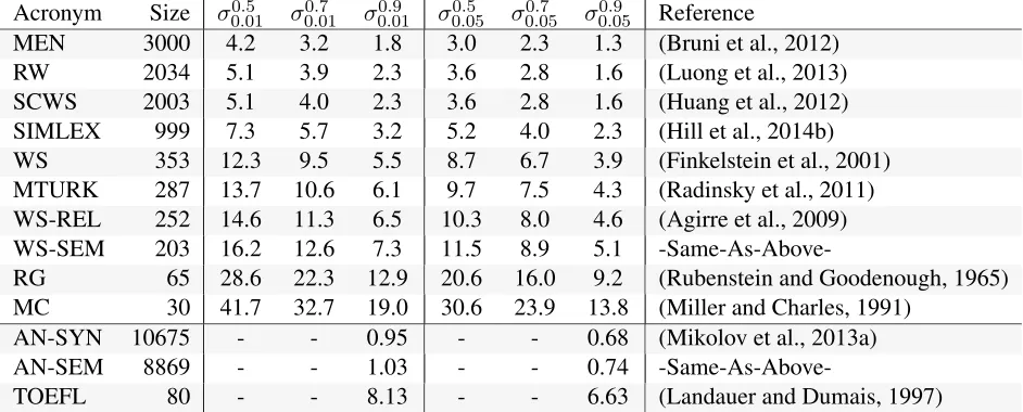
Test DataWe evaluated the representations on the word similarity datasets listed in Table 2. The first 10 datasets in Table 2 were annotated with different rubrics and rated on different scales. But broadly they all contain human judgements about how simi-lar two words are. The “AN-SYN” and “AN-SEM” datasets contain 4-tuples of analogous words and the
2Dependency relations employed: nsubj, amod, advmod,
rcmod, dobj, prep of, prep in, prep to, prep on, prep for, prep with, prep from, prep at, prep by, prep as, prep between, xsubj, agent, conj and, conj but, pobj.
Embeddings (Incremental, Missing value aware, Max-‐Var
GCCA)
Monolingual Text From Wikipedia
Word Aligned Bitext (Fr, Zh, Es, De, …)
Dependency RelaKons (nsubj, amod,
advmod, …) Morphology (CatVar, Morphy/a)
[image:4.612.316.537.65.197.2]Frame RelaKons (FrameNet)
Figure 1: An illustration of datasets used.
Language Sentences English Tokens
Bitext-Arabic 8.8M 190M
Bitext-Czech 7.3M 17M
Bitext-German 1.8M 44M
Bitext-Spanish 11.1M 241M
Bitext-French 30.9M 671M
Bitext-Chinese 10.3M 215M
Monotext-En-Wiki 75M 1700M
Table 1: Portion of data used to create GCCA representa-tions (in millions).
task is to predict the missing word given the first three. Both of these are open vocabulary tasks while TOEFL is a closed vocabulary task.
4.1 Significance of comparison
While surveying the literature we found that perfor-mance on word similarity datasets is typically re-ported in terms of the Spearman correlation between the gold ratings and the cosine distance between nor-malized embeddings. However researchers do not report measures of significance of the difference be-tween the Spearman Correlations even for
compar-isons on small evaluation sets.3 This motivated our
defining a method for calculating theMinimum
Re-quired Difference for Significance (MRDS).
Minimum Required Difference for Significance (MRDS): Imagine two lists of ratings over the same
3For example, the comparative difference by competing
Acronym Size σ0.5
0.01 σ0.010.7 σ0.90.01 σ0.50.05 σ0.050.7 σ0.050.9 Reference
MEN 3000 4.2 3.2 1.8 3.0 2.3 1.3 (Bruni et al., 2012)
RW 2034 5.1 3.9 2.3 3.6 2.8 1.6 (Luong et al., 2013)
SCWS 2003 5.1 4.0 2.3 3.6 2.8 1.6 (Huang et al., 2012)
SIMLEX 999 7.3 5.7 3.2 5.2 4.0 2.3 (Hill et al., 2014b)
WS 353 12.3 9.5 5.5 8.7 6.7 3.9 (Finkelstein et al., 2001)
MTURK 287 13.7 10.6 6.1 9.7 7.5 4.3 (Radinsky et al., 2011)
WS-REL 252 14.6 11.3 6.5 10.3 8.0 4.6 (Agirre et al., 2009)
WS-SEM 203 16.2 12.6 7.3 11.5 8.9 5.1
-Same-As-Above-RG 65 28.6 22.3 12.9 20.6 16.0 9.2 (Rubenstein and Goodenough, 1965)
MC 30 41.7 32.7 19.0 30.6 23.9 13.8 (Miller and Charles, 1991)
AN-SYN 10675 - - 0.95 - - 0.68 (Mikolov et al., 2013a)
AN-SEM 8869 - - 1.03 - - 0.74
[image:5.612.72.543.58.248.2]-Same-As-Above-TOEFL 80 - - 8.13 - - 6.63 (Landauer and Dumais, 1997)
Table 2: List of test datasets used. The columns headedσr
p0 containMRDSvalues. The rows for accuracy based test
sets containσp0which does not depend onr. See§4.1 for details.
items, produced respectively by algorithms A and
B, and then a list of gold ratings T. Let rAT,
rBT andrAB denote the Spearman correlations
be-tween A : T, B : T andA : B respectively. Let
ˆ
rAT,rˆBT,rˆAB be their empirical estimates and
as-sume thatrˆBT >ˆrAT without loss of generality.
For word similarity datasets we defineσr
p0 as the MRDS, such that it satisfies the following proposi-tion:
(rAB< r)∧(|ˆrBT −ˆrAT|<σpr0) =⇒pval> p0
. Here pval is the probability of the test statistic
under the null hypothesis that rAT = rBT found
using the Steiger’s test (Steiger, 1980). The above constraint ensures that as long as the correlation
be-tween the competing methods is less thanrand the
difference between the correlations of the scores of the competing methods to the gold ratings is less thanσr
p0, then the pvalue of the null hypothesis will
be greater thanp0. We can then ask what we
con-sider a reasonable upper bound on the agreement of ratings produced by competing algorithms: for
in-stance two algorithms correlating above 0.9 might
not be considered meaningfully different. That leaves us with the second part of the predicate which ensures that as long as the difference between the correlations of the competing algorithms to the gold
scores is less than σr
p0 then the null hypothesis is
more likely thanp0.
We can find σr
p0 as follows: Let stest denote
Steiger’s test predicate which satisfies the following:
stest-p(ˆrAT,rˆBT, rAB, p0, n) =⇒pval< p0
Once we define this predicate then we can use it to set up an optimistic problem where our aim is to find
σr
p0 by solving the following:
σr
p0= min{σ|∀0<r0<1stest-p(r0,min(r0+σ,1), r, p0, n)}
Note that MRDS is a liberal threshold and it only guarantees that differences in correlations below that threshold can never be statistically significant (un-der the given parameter settings). MRDS might op-timistically consider some differences as significant when they are not, but it is at least useful in reducing some of the noise in the evaluations. The values of
σr
p0 are shown in Table 2.
For the accuracy based test-sets we found
MRDS=σp0 that satisfied the following:
0<(ˆθB−θˆA)< σp0 =⇒p(θB≤θA)> p0
Specifically, we calculated the posterior probabil-ity p(θB ≤ θA)with a flat prior of β(1,1)to solve
the following:4 σ
p0 = min{σ|∀0<θ<min(1−σ,0.9)
p(θB≤θA|θˆA=θ,θˆB=θ+σ, n)< p0}HereθAandθB
4This instead of using McNemar’s test (McNemar, 1947)
since the Bayesian approach is tractable and more direct. A cal-culation withβ(0.5,0.5)as the prior changedσ0.5 from 6.63
are probability of correctness of algorithms A, B
andθˆA,θˆBare observed empirical accuracies.
Unfortunately there are no widely reported train-test splits of the above datasets, leading to potential
concerns of soft supervision (hyper-parameter
tun-ing) on these evaluations, both in our own work and throughout the existing literature. We report on the resulting impact of various parameterizations, and our final results are based on a single set of parame-ters used across all evaluation sets.
5 Experiments and Results
We wanted to answer the following questions through our experiments: (1) How do hyper-parameters affect performance? (2) What is the con-tribution of the multiple sources of data to perfor-mance? (3) How does the performance of MVLSA compare with other methods? For brevity we show tuning runs only on the larger datasets. We also highlight the top performing configurations in bold
using the small threshold values in columnσ0.09
0.05 of
Table 2.
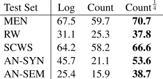
Effect of Hyper-parameters fj: We modeled the
preprocessing functionfj as the composition of two
functions, fj = nj ◦tj. nj represents nonlinear
preprocessing that is usually employed with LSA.
We experimented by settingnjto be: identity;
loga-rithm of count plus one; and the fourth root of the
count. tj represents the truncation of columns
and can be interpreted as a type of regularization of the raw counts themselves through which we prune
away the noisy contexts. Decrease intjalso reduces
[image:6.612.317.544.57.128.2]the influence of views that have a large number of context columns and emphasizes the sparser views. Table 3 and Table 4 show the results.
Test Set Log Count Count14
MEN 67.5 59.7 70.7
RW 31.1 25.3 37.8
SCWS 64.2 58.2 66.6
AN-SYN 45.7 21.1 53.6
AN-SEM 25.4 15.9 38.7
Table 3: Performance versusnj, the non linear
process-ing of cooccurrence counts.t = 200K, m = 500, v = 16, k = 300. All the top configurations determined by σ0.09
0.05are in bold font.
Test Set 6.25K 12.5K 25K 50K 100K 200K MEN 70.2 71.2 71.5 71.6 71.2 70.7
RW 41.8 41.7 41.5 40.9 39.6 37.8 SCWS 67.1 67.3 67.1 67.0 66.9 66.6
AN-SYN 59.2 60.0 59.5 58.4 56.1 53.6 AN-SEM 37.7 38.6 39.4 39.2 38.4 38.7
Table 4: Performance versus the truncation threshold,t, of raw cooccurrence counts. We usednj =Count14 and
other settings were the same as Table 3.
m: The number of left singular vectors extracted
after SVD of the preprocessed cooccurrence matri-ces can again be interpreted as a type of regular-ization, since the result of this truncation is that we find cooccurrence patterns only between the top left
singular vectors. We set mj = max(dj, m) with
m= [100,300,500]. See table 5.
Test Set 100 200 300 500
MEN 65.6 68.5 70.1 71.1
RW 34.6 36.0 37.2 37.1
SCWS 64.2 65.4 66.4 66.5
AN-SYN 50.5 56.2 56.4 56.4
AN-SEM 24.3 31.4 34.3 40.6
Table 5: Performance versusm, the number of left singu-lar vectors extracted from raw cooccurrence counts. We setnj =Count14, t= 100K, v= 25, k= 300.
k: Table 6 demonstrates the variation in
perfor-mance versus the dimensionality of the learnt vec-tor representations of the words. Since the dimen-sions of the MVLSA representations are orthogonal to each other therefore creating lower dimensional representations is a trivial matrix slicing operation and does not require retraining.
Test Set 10 50 100 200 300 500
MEN 49.0 67.0 69.7 70.2 70.1 69.8
RW 28.8 33.3 35.0 35.2 37.2 38.3
SCWS 57.8 64.4 65.2 66.1 66.4 65.1
AN-SYN 9.0 41.2 52.2 55.4 56.4 54.4
[image:6.612.315.553.544.626.2]AN-SEM 2.5 21.8 34.8 35.8 34.3 33.8
Table 6: Performance versusk, the final dimensionality of the embeddings. We setm = 300and other settings were same as Table 5.
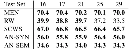
v: Expression 12 describes a method to setWj.
[image:6.612.103.269.553.634.2]heuristic to set [Wj]ii = (Kww ≥ v), essentially
removing all words that did not appear in v views
before doing GCCA. Table 7 shows that changes in
vare largely inconsequential for performance.
Test Set 16 17 21 25 29
MEN 70.4 70.4 70.2 70.1 70.0
RW 39.9 38.8 39.7 37.2 33.5
SCWS 67.0 66.8 66.5 66.4 65.7
AN-SYN 56.0 55.8 55.9 56.4 56.0
AN-SEM 34.6 34.3 34.0 34.3 34.3
Table 7: Performance versus minimum view support threshold v, The other hyperparameters were nj =
Count14, m = 300, t = 100K. Though a clear best
setting did not emerge, we chosev = 25as the middle ground.
rj: The regularization parameter ensures that all
the inverses exist at all points in our method. We found that the performance of our procedure was
in-variant torover a large range from 1 to 1e-10. This
was because even the 1000th singular value of our data was much higher than 1.
Contribution of different sources of dataTable 8 shows an ablative analysis of performance where we remove individual views or some combination of them and measure the performance. It is clear by comparing the last column to the second column that adding in more views improves performance. Also we can see that the Dependency based views and the Bitext based views give a larger boost than the mor-phology and FrameNet based views, probably be-cause the latter are so sparse.
Comparison to other word representation cre-ation methods There are a large number of meth-ods of creating representations both multilingual and monolingual. There are many new methods such as by Yu and Dredze (2014), Faruqui et al. (2014), Hill and Korhonen (2014), and Weston et al. (2014) that are performing multiview learning and could be con-sidered here as baselines: however it is not straight-forward to use those systems to handle the variety of data that we are using. Therefore, we directly compare our method to the Glove and the SkipGram model of Word2Vec as the performance of those sys-tems is considered state of the art. We trained these
two systems on the English portion of thePolyglot
Wikipedia dataset.5 We also combined their outputs
using MVLSA to createMV-G-WSG)embeddings.
We trained our best MVLSA system with data from all views and by using the individual best settings of the hyper-parameters. Specifically the
configuration we used was as follows: nj =
Count14, t = 12.5K, m = 500, k = 300, v = 16.
To make a fair comparison we also provide results
where we used only the views derived from the
Poly-glot Wikipedia corpus. See column MVLSA (All
Views)andMVLSA (Wiki)respectively. It is clearly visible that MVLSA on the monolingual data itself is competitive with Glove but worse than Word2Vec on the word similarity datasets and it is substan-tially worse than both the systems on the AN-SYN and AN-SEM datasets. However with the addition of multiple views MVLSA makes substantial gains,
shown in columnMV Gain, and after consuming the
Glove and WSG embeddings it again improves
per-formance by some margins, as shown in column
G-WSG Gain, and outperforms the original systems. Using GCCA itself for system combination provides closure for the MVLSA algorithm since multiple distinct approaches can now be simply fused using this method. Finally we contrast the Spearman
cor-relations rs with Glove and Word2Vec before and
after including them in the GCCA procedure. The values demonstrate that including Glove and WSG during GCCA actually increased the correlation be-tween them and the learnt embeddings, which sup-ports our motivation for performing GCCA in the first place.
6 Previous Work
Vector space representations of words have been cre-ated using diverse frameworks including Spectral methods (Dhillon et al., 2011; Dhillon et al., 2012),
6 Neural Networks (Mikolov et al., 2013b;
Col-lobert and Lebret, 2013), and Random Projections (Ravichandran et al., 2005; Bhagat and
Ravichan-5We explicitly provided the vocabulary file to Glove and
Word2Vec and set the truncation threshold for Word2Vec to 10. Glove was trained for 25 iterations. Glove was provided a window of 15 previous words and Word2Vec used a symmet-ric window of 10 words.
[image:7.612.80.291.127.208.2]Test Set Views !Framenet !Morphology !Bitext !Wikipedia !DependencyAll !Morphology!Framenet !Morphology!Framenet !Bitext
MEN 70.1 69.8 70.1 69.9 46.4 68.4 69.5 68.4
RW 37.2 36.4 36.1 32.2 11.6 34.9 34.1 27.1
SCWS 66.4 65.8 66.3 64.2 54.5 65.5 65.2 60.8
AN-SYN 56.4 56.3 56.2 51.2 37.6 50.5 54.4 46.0
[image:8.612.75.540.223.420.2]AN-SEM 34.3 34.3 34.3 36.2 4.1 35.3 34.5 30.6
Table 8: Performance versus views removed from the multiview GCCA procedure. !Framenet means that the view containing counts derived from Frame semantic dataset was removed. Other columns are named similarly. The other hyperparameters werenj=Count14, m= 300, t= 100K, v= 25, k= 300.
Test Set Glove WSG MV MVLSA MVLSA MVLSA MV G-WSG rsMVLSA rsMV-G-WSG
G-WSG Wiki All Views Combined Gain Gain Glove WSG Glove WSG
MEN 70.4 73.9 76.0 71.4 71.2 75.8 −0.2 4.6† 71.9 89.1 85.8 92.3
RW 28.1 32.9 37.2 29.0 41.7 40.5 12.7† −1.2 72.3 74.2 80.2 75.6
SCWS 54.1 65.6 60.7 61.8 67.3 66.4 5.5† −0.9 87.1 94.5 91.3 96.3
SIMLEX 33.7 36.7 41.1 34.5 42.4 43.9 7.9† 1.5 62.4 78.2 79.3 86.0
WS 58.6 70.8 67.4 68.0 70.8 70.1 2.8† −0.7 72.3 88.1 81.8 91.8
MTURK 61.7 65.1 59.8 59.1 59.7 62.9 0.6 3.2 80.0 87.7 87.3 92.5
WS-REL 53.4 63.6 59.6 60.1 65.1 63.5 5.0† −1.6 58.2 81.0 69.6 85.3
WS-SEM 69.0 78.4 76.1 76.8 78.8 79.2 2.0 0.4 74.4 90.6 83.9 94.0
RG 73.8 78.2 80.4 71.2 74.4 80.8 3.2 6.4† 80.3 90.6 91.8 92.9
MC 70.5 78.5 82.7 76.6 75.9 77.7 −0.7 2.8 80.1 94.1 91.4 95.8
AN-SYN 61.8 59.8 51.0 42.7 60.0 64.3 17.3† 4.3†
AN-SEM 80.9 73.7 73.5 36.2 38.6 77.2 2.4† 38.6†
TOEFL 83.8 81.2 86.2 78.8 87.5 88.8 8.7† 1.3
Table 9: Comparison of Multiview LSA against Glove and WSG(Word2Vec Skip Gram). Usingσ0.9
0.05as the threshold
we highlighted the top performing systems in bold font. †marks significant increments in performance due to use of multiple views in theGaincolumns. Therscolumns demonstrate that GCCA increased pearson correlation.
dran, 2008; Chan et al., 2011). 7 They have been
trained using either one (Pennington et al., 2014)8
or two sources of cooccurrence statistics (Zou et al., 2013; Faruqui and Dyer, 2014; Bansal et al., 2014;
Levy and Goldberg, 2014) 9 or using multi-modal
data (Hill and Korhonen, 2014; Bruni et al., 2012). Dhillon et al. (2011) and Dhillon et al. (2012) were the first to use CCA as the primary method to learn vector representations and Faruqui and Dyer (2014) further demonstrated that
incorporat-7code.google.com/p/
word2vec,metaoptimize.com/projects/ wordreprs
8nlp.stanford.edu/projects/glove 9ttic.uchicago.edu/˜mbansal/data/
syntacticEmbeddings.zip,cs.cmu.edu/ ˜mfaruqui/soft.html
ing bilingual data through CCA improved perfor-mance. More recently this same phenomenon was reported by Hill et al. (2014a) through their exper-iments over neural representations learnt from MT systems. Various other researchers have tried to im-prove the performance of their paraphrase systems or vector space models by using diverse sources of information such as bilingual corpora (Bannard and Callison-Burch, 2005; Huang et al., 2012; Zou et al.,
2013),10 structured datasets (Yu and Dredze, 2014;
Faruqui et al., 2014) or even tagged images (Bruni
10An example of complementary views: Chan et al. (2011)
et al., 2012). However, most previous work11 did
not adopt the general, simplifying view that all of these sources of data are just cooccurrence statistics coming from different sources with underlying la-tent factors.12
Bach and Jordan (2005) presented a probabilistic interpretation for CCA. Though they did not gener-alize it to include GCCA we believe that one could
give a probabilistic interpretation of MAX-VAR
GCCA. Such a probabilistic interpretation would
al-low for an online-generative model of lexical repre-sentations, which unlike methods like Glove or LSA would allows us to naturally perplexity or generate sequences. We also note that V´ıa et al. (2007) pre-sented a neural network model of GCCA and adap-tive/incremental GCCA. To the best of our knowl-edge both of these approaches have not been used for word representation learning.
CCA is also an algorithm for multi-view learning (Kakade and Foster, 2007; Ganchev et al., 2008) and when we view our work as an application of multi-view learning to NLP, this follows a long chain of ef-fort started by Yarowsky (1995) and continued with
Co-Training (Blum and Mitchell, 1998),
CoBoost-ing (Collins and Singer, 1999) and 2 view
percep-trons(Brefeld et al., 2006).
7 Conclusion and Future Work
While previous efforts demonstrated that incorporat-ing two views is beneficial in word-representation learning, we extended that thread of work to a
logical extreme and created MVLSA to learn
dis-tributed representations using data from 46 views!13
Through evaluation of our induced representations, shown in Table 9, we demonstrated that the MVLSA algorithm is able to leverage the information present in multiple data sources to improve performance on a battery of tests against state of the art baselines. In order to perform MVLSA on large vocabularies
11Ganitkevitch et al. (2013) did employ a rich set of
di-verse cooccurrence statistics in constructing the initial PPDB, but without a notion of “training” a joint representation beyond random projection to a binary vector subspace (bit-signatures).
12Note that while Faruqui et al. (2014) performed belief
prop-agation over a graph representation of their data, such an undi-rected weighted graph can be viewed as an adjacency matrix, which is then also a cooccurrence matrix.
13Code and data available at www.cs.jhu.edu/
˜prastog3/mvlsa
with up to 500K words we presented a fast scalable algorithm. We also showed that a close variant of the Glove objective proposed by Pennington et al. (2014) could be derived as a heuristic for handling missing data under the MVLSA framework. In or-der to better unor-derstand the benefit of using mul-tiple sources of data we performed MVLSA using views derived only from the monolingual Wikipedia dataset thereby providing a more principled alterna-tive of LSA that removes the need for heuristically combining word-word cooccurrence matrices into a single matrix. Finally, while surveying the litera-ture we noticed that not enough emphasis was being given towards establishing the significance of
com-parative results and proposed a method, (MRDS),
to filter out insignificant comparative gains between competing algorithms.
Future Work Column MVLSA Wiki of Table 9 shows us that MVLSA applied to monolingual data has mediocre performance compared to the base-lines of Glove and Word2Vec on word similarity tasks and performs surprisingly worse on the AN-SEM dataset. We believe that the results could be improved by (1) either using recent methods for handling missing values mentioned in footnote 1 or by using the heuristic count dependent non-linear weighting mentioned by Pennington et al. (2014) and that sits well within our framework as exempli-fied in Expression 12 (2) by using even more views, which look at the future words as well as views that contain PMI values. Finally, we note that Table 8 shows that certain datasets can actually degrade per-formance over certain metrics. Therefore we are ex-ploring methods for performing discriminative opti-mization of weights assigned to views, for purposes of task-based customization of learned representa-tions.
Acknowledgments
References
Eneko Agirre, Enrique Alfonseca, Keith Hall, Jana Kravalova, Marius Pas¸ca, and Aitor Soroa. 2009. A study on similarity and relatedness using distribu-tional and wordnet-based approaches. InProceedings of NAACL-HLT. ACL.
Rami Al-Rfou, Bryan Perozzi, and Steven Skiena. 2013. Polyglot: Distributed word representations for multi-lingual nlp. InProceedings of CoNLL. ACL.
Animashree Anandkumar, Rong Ge, Daniel Hsu, Sham M. Kakade, and Matus Telgarsky. 2014. Ten-sor decompositions for learning latent variable models. JMLR, 15.
Raman Arora and Karen Livescu. 2012. Kernel CCA for multi-view learning of acoustic features using articu-latory measurements. MLSLP.
Francis R Bach and Michael I Jordan. 2005. A prob-abilistic interpretation of canonical correlation analy-sis. Technical Report 688, Department of Statistics, University of California, Berkeley.
Colin Bannard and Chris Callison-Burch. 2005. Para-phrasing with bilingual parallel corpora. In Proceed-ings of ACL. ACL.
Mohit Bansal, Kevin Gimpel, and Karen Livescu. 2014. Tailoring continuous word representations for depen-dency parsing. InProceedings of ACL. ACL.
Rahul Bhagat and Deepak Ravichandran. 2008. Large scale acquisition of paraphrases for learning surface patterns. InProceedings of ACL-HLT.
Avrim Blum and Tom Mitchell. 1998. Combining la-beled and unlala-beled data with co-training. In Proceed-ings of COLT. ACM.
Matthew Brand. 2002. Incremental singular value de-composition of uncertain data with missing values. In Computer Vision—ECCV 2002, pages 707–720. Springer.
Matthew Brand. 2006. Fast low-rank modifications of the thin singular value decomposition.Linear algebra and its applications, 415(1).
Ulf Brefeld, Thomas G¨artner, Tobias Scheffer, and Stefan Wrobel. 2006. Efficient co-regularised least squares regression. InProceedings of ICML. ACM.
Elia Bruni, Gemma Boleda, Marco Baroni, and Nam-Khanh Tran. 2012. Distributional semantics in tech-nicolor. InProceedings of ACL. ACL.
J Douglas Carroll. 1968. Generalization of canonical correlation analysis to three or more sets of variables. InProceedings of APA, volume 3.
Tsz Ping Chan, Chris Callison-Burch, and Benjamin Van Durme. 2011. Reranking bilingually extracted para-phrases using monolingual distributional similarity. In Proceedings of EMNLP Workshop: GEMS.
Michael Collins and Yoram Singer. 1999. Unsupervised models for named entity classification. InProceedings of EMNLP. ACL.
Ronan Collobert and R´emi Lebret. 2013. Word embed-dings through hellinger pca. Technical report, Idiap. Paramveer Dhillon, Dean Foster, and Lyle Ungar. 2011.
Multi-view learning of word embeddings via CCA. In Procesdings of NIPS.
Paramveer Dhillon, Jordan Rodu, Dean P Foster, and Lyle H Ungar. 2012. Two step CCA: A new spec-tral method for estimating vector models of words. In Proceedings of ICML. ACM.
Manaal Faruqui and Chris Dyer. 2014. Improving vector space word representations using multilingual correla-tion. InProceedings of EACL.
Manaal Faruqui, Jesse Dodge, Sujay Jauhar, Chris Dyer, Eduard Hovy, and Noah Smith. 2014. Retrofitting word vectors to semantic lexicons. InProceedings of the deep learning and representation learning work-shop, NIPS.
Lev Finkelstein, Evgeniy Gabrilovich, Yossi Matias, Ehud Rivlin, Zach Solan, Gadi Wolfman, and Eytan Ruppin. 2001. Placing search in context: The concept revisited. InProceedings of WWW. ACM.
Kuzman Ganchev, Joao Graca, John Blitzer, and Ben Taskar. 2008. Multi-view learning over structured and non-identical outputs. InProceedings of UAI.
Juri Ganitkevitch, Benjamin Van Durme, and Chris Callison-Burch. 2013. Ppdb: The paraphrase database. InProceedings of NAACL-HLT.
Nizar Habash and Bonnie Dorr. 2003. Catvar: A database of categorial variations for english. In Pro-ceedings of MT Summit.
Trevor Hastie, Robert Tibshirani, and Jerome Friedman. 2009.The Elements Of Statistical Learning, volume 2. Springer.
Felix Hill and Anna Korhonen. 2014. Learning abstract concept embeddings from multi-modal data: Since you probably can’t see what i mean. InProceedings of EMNLP. ACL.
Felix Hill, KyungHyun Cho, Sebastien Jean, Coline Devin, and Yoshua Bengio. 2014a. Not all neu-ral embeddings are born equal. arXiv preprint arXiv:1410.0718.
Felix Hill, Roi Reichart, and Anna Korhonen. 2014b. Simlex-999: Evaluating semantic models with (genuine) similarity estimation. arXiv preprint arXiv:1408.3456.
Eric H. Huang, Richard Socher, Christopher D. Manning, and Andrew Y. Ng. 2012. Improving word representa-tions via global context and multiple word prototypes. InProceedings of ACL. ACL.
Sham M Kakade and Dean P Foster. 2007. Multi-view regression via canonical correlation analysis. In Learning Theory. Springer.
Jon R Kettenring. 1971. Canonical analysis of several sets of variables.Biometrika, 58(3):433–451.
Thomas K Landauer and Susan T Dumais. 1997. A so-lution to plato’s problem: The latent semantic analysis theory of acquisition, induction, and representation of knowledge. Psychological review, 104(2):211. Omer Levy and Yoav Goldberg. 2014.
Dependency-based word embeddings. In Proceedings of ACL. ACL.
Minh-Thang Luong, Richard Socher, and Christopher D. Manning. 2013. Better word representations with re-cursive neural networks for morphology. In Proceed-ings of CoNLL. ACL.
Quinn McNemar. 1947. Note on the sampling error of the difference between correlated proportions or per-centages. Psychometrika, 12(2).
Tomas Mikolov, Ilya Sutskever, Kai Chen, Greg Corrado, and Jeff Dean. 2013a. Distributed representations of words and phrases and their compositionality. In Pro-ceedings of NIPS.
Tomas Mikolov, Wen-tau Yih, and Geoffrey Zweig. 2013b. Linguistic regularities in continuous space word representations. InProceedings of NAACL-HLT, pages 746–751.
George A. Miller and Walter G. Charles. 1991. Contex-tual correlates of semantic similarity. Language and Cognitive Processes, 6(1).
Guido Minnen, John Carroll, and Darren Pearce. 2001. Applied morphological processing of english. Natural Language Engineering, 7(03).
Courtney Napoles, Matthew Gormley, and Benjamin Van Durme. 2012. Annotated gigaword. InProceedings of NAACL Workshop: AKBC-WEKEX.
Jeffrey Pennington, Richard Socher, and Christopher D. Manning. 2014. Glove: global vectors for word rep-resentation. InProceedings of EMNLP. ACL.
Kira Radinsky, Eugene Agichtein, Evgeniy Gabrilovich, and Shaul Markovitch. 2011. A word at a time: Com-puting word relatedness using temporal semantic anal-ysis. InProceedings of WWW. ACM.
Pushpendre Rastogi and Benjamin Van Durme. 2014. Augmenting framenet via PPDB. In Proceedings of the Second Workshop on EVENTS: Definition, Detec-tion, Coreference, and Representation. ACL.
Deepak Ravichandran, Patrick Pantel, and Eduard Hovy. 2005. Randomized algorithms and nlp: Using locality
sensitive hash functions for high speed noun cluster-ing. InProceedings of ACL.
Herbert Rubenstein and John B. Goodenough. 1965. Contextual correlates of synonymy. Communications of the ACM, 8(10).
Dmitry Savostyanov. 2014. Efficient way to find svd of sum of projection matrices? MathOver-flow. URL:http://mathoverMathOver-flow.net/q/178573 (version: 2014-08-14).
Karthik Sridharan and Sham M Kakade. 2008. An infor-mation theoretic framework for multi-view learning. InProceedings of COLT.
James H Steiger. 1980. Tests for comparing elements of a correlation matrix.Psychological Bulletin, 87(2). Peter D Turney and Patrick Pantel. 2010. From
fre-quency to meaning: Vector space models of semantics. Journal of AI Research, 37(1).
Michel Van De Velden and Tammo HA Bijmolt. 2006. Generalized canonical correlation analysis of matrices with missing rows: a simulation study. Psychome-trika, 71(2).
Michel van de Velden and Yoshio Takane. 2012. Gener-alized canonical correlation analysis with missing val-ues.Computational Statistics, 27(3).
Javier V´ıa, Ignacio Santamar´ıa, and Jes´us P´erez. 2007. A learning algorithm for adaptive canonical correlation analysis of several data sets. Neural Networks, 20(1). Jason Weston, Sumit Chopra, and Keith Adams. 2014.
#tagspace: Semantic embeddings from hashtags. In Proceedings of EMNLP, Doha, Qatar. ACL.
Terry Winograd. 1972. Understanding natural language. Cognitive psychology, 3(1):1–191.
David Yarowsky. 1995. Unsupervised WSD rivaling su-pervised methods. InProceedings of ACL. ACL. Mo Yu and Mark Dredze. 2014. Improving lexical
em-beddings with semantic knowledge. InProceedings of ACL. ACL.