A Method of Incorporating Bigram Constraints into an LR Table and Its Effectiveness in Natural Language Processing

(1)

II

A M e t h o d of Incorporating Bigram Constraints into an LR

Table and Its Effectiveness in Natural Language Processing

i

Hiroki

Imai and Hozumi Tanaka

Graduate School of Information Science and Technology

Tokyo Institute of Technology

2-12-10-okayama, Meguro, Tokyo 152 Japan

{ i m a i , t a n a k a } @ c s , t i t e c h , ac. j p

Abstract

In this paper, we propose a method for con- structing bigram LR tables by way of incorporating bigram constraints into an LR table. Using a bigram LR table, it is possible for a GLR parser to make use of both big'ram and CFG constraints in natural language processing.

Applying bigram LR tables to our GLR method has the following advantages: (1) Language models utilizing bigzam LR tables have lower perplexity than simple bigram language models, since local constraints (hi- gram) and global constraints (CFG) are com- bined in a single bigram LR table.

(2) Bigram constraints are easily acquired from a given corpus. Therefore data sparseness is not likely to arise.

(3) Separation of local and global constraints keeps down the number of CFG rules. The first advantage leads to a reduction in complexity, and as the result, better performance in GLR parsing.

Our experiments demonstrate the effectiveness

of our method.

1 Introduction

In natural language processing, stochastic language models are commonly used for lexical and syntactic disambiguation (Fujisaki et al., 1991; Franz, 1996). Stochastic language models are also helpful in re- ducing the complexity of speech and language processing by way of providing probabilistic linguistic constraints (Lee, 1989).

N-gram language models (Jelinek, 1990), includ- ing bigram and trigram models, are the most commonly used method of applying local probabilistic constraints. However, context-free grammars (CFGs) produce more global linguistic constraints than N-gram models. It seems better to combine both local and global constraints and use them both concurrently in natural language processing. The reason why N-gram models are preferred over CFGs is that N-gram constraints are easily acquired from

a given corpus. However, the larger N is, the more serious the problem of data sparseness becomes.

CFGs are commonly employed in syntactic parsing as global linguistic constraints, since many eifi- cient parsing algorithms are available. GLR (Gen- eralized LR) is one such parsing algorithm that uses an LR table, into which CFG constraints are pre- compiled in advance (Knuth, 1965; Tomita, 1986). Therefore if we can incorporate N-gram constraints into an LR table, we can make concurrent use of both local and global linguistic constraints in GLR parsing.

In the following section, we will propose a method that incorporates bigram constraints into an LR table. The advantages of the method are summarized as follows:

First, it is expected that this method produces a lower perplexity than that for a simple bigram language model, since it is possible to utilize both local (bigram) and global (CFG) constraints in the LR table. We will evidence this reduction in perplexity by considering states in an LR table for the case of GLR parsing.

Second, bigram constraints are easily acquired from smaller-sized corpora. Accordingly, data sparseness is not likely to arise.

Third, the separation of local and global constraints makes it easy to describe CFG rules, since CFG writers need not take into'account tedious de- scriptions of local connection constraints within th C F G I .

2 CFG, Connection Matrix a n d L R

table

2.1 R e l a t i o n b e t w e e n C F G and C o n n e c t i o n

C o n s t r a i n t s

Figure 1 represents a situation in which ai and bj are adjacent to each other, where a~ belongs to S e t l (i = 1 , . . - , I ) and bj belongs to S e t j (j = 1 , . . . , J). Set~

l(Tana~ et al., 1997) reported that the separate description of local and global constraints reduced the CFG rules to one sixth of their original number.

Imai and Tanaka 225 A Method of Incorporating Bigram Constraints

(2)

X

Y

Z

[image:2.612.340.503.57.249.2]

b j

Figure 1: Connection check by C F G

and Sets are defined by last1 (Y) and first1 ( Z) (Aho et al., 1986), respectively. If a E Setz and b E Sets happen not to be able to occur in this order, it becomes a non-trivial task to express this adjacency restriction within the framework of a CFG.

One solution to this problem is to introduce a new nonterminal symbol

Ai

for each a~ and a nonterminal symbol Bj for each hi. We then add rules of the form A --* Ai and Ai "* ai, and B ~ Bj and B i --* bj. As a result of this rule expansion, the order of the number of rules will become I x J in the worst case. The introduction of such new nonterminal symbols leads to an increase in g r a m m a r rules, which not only makes the LR table very large in size, but also diminishes efficiency of the G L R parsing method.

The second solution is to augment X ~ Y Z with a procedure that checks the connection between a~ and bj. This solution can avoid the problem of the expansion of CFG rules, but we have to take care of the information flow from the bottom leaves to the upper nodes in the tree, Y, Z, and X.

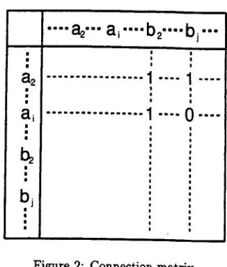
Neither the first nor the second solution are prefer- able, in terms of both efficiency of GLR parsing and description of CFG rules. Additionally, it is a much easier task to describe local connection constraints between two adjacent terminal symbols by way of a connection matrix such as in Figure 2, than to express these constraints within the CFG.

The connection matrix in Figure 2 is defined as:

= { ~ if bj can follow ai

Connect( a~, bj ) _otherwise ₍₁₎

The best solution seems to be to develop a method that can combine both a C F G and a connection matrix, avoiding the expansion of CFG rules. Conse- quently, the size of the LR table will become smaller and we will get better G L R parsing performance. In the following section, we will propose one such method. Note that we are considering connections between preterminals rather than words. Thus, we will have Connect(ai, bj) = 0 in the preterminal connection matrix similarly to the case of words.

a2

a~

I

• "-- . . . . b j . - -

I a

I I

I i

I . . . . I ....

! |

o |

e I

--1 . . . . 0 ....

| |

I i

o |

i e

o j

i e

f I

| |

I i

| |

= |

I s

t |

| I

| |

| I

| i

Figure 2: Connection matrix

2.2 R e l a t i o n b e t w e e n t h e LR Table a n d

C o n n e c t i o n M a t r i x

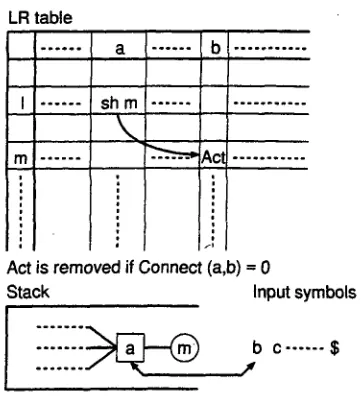
First we discuss the relation between the LR table and a connection matrix. The action part of an LR table consists of lookahead symbols and states. Let a shift action sh m be in state l with the lookahead symbol a. After the GLR parser executes action sh m, the symbol a is pushed onto the top of the stack and the GLR parser shifts to state m. Sup- pose there is an action A in state m with lookahead b (see Figure 3). The action A is executable if Connect(a,b) ~ 0 (b can follow a), whereas if Connect(a, b) = 0 (b cannot follow a), the action A in state m with lookahead b is not executable and we can remove it from the LR table as an invalid action. Removing such invalid actions enables us to incorporate connection constraints into the LR table in addition to the implicit CFG constraints.

In section 3.2, we will propose a method that in- tegrates both bigram and CFG constraints into an LR table. After this integration process, we obtain a table called a bigram LR table.

3 I n t e g r a t i o n o f B i g r a m a n d C F G C o n s t r a i n t s i n t o a n L R T a b l e

3.1 T h e Definition o f a Probabilistic

C o n n e c t i o n M a t r i x

A close relation exists between bigrams and connection matrices, in that the bigram probability P(bla ) corresponds to the matrix dement of Connect(a, b). A connection matrix incorporating bigram probabilities is called a probabilistic connection matrix, in which Connect(a, b) = 0 still means b cannot follow a, but instead of connection matrix entries having a binary value of 0 or 1, a probability is associated with each element. This is then used to construct a probabilistic LR table.

I

II

[image:2.612.123.286.60.181.2]

(3)

II

m

m m

LR table

• ° . o ° ° ° ,

I | . . . '

m . . .

a sh m

\

' = ° ° = = " ' b , . . . . ~ . . .

Acl . . .

Act is removed if Connect (a,b) = 0

Stack Input symbols

Figure 3: LR table and Connection Constraints

The N-gram model is the most commonly used probabilistic language model, and it assumes that a symbol sequence can be described by a higher order Markov process. The simplest N-gram model with N = 2 is called a bigram model, and approximates the probability of a string X = xzx2xa...x,~ as the product of conditional probabilities:

P ( X ) = e ( x z l # ) P ( x 2 l x l ) . . . P(x=lx=-l)P($1x,) (2) In the above expression, " # " indicates the sentence beginning marker and "$" indicates the sentence ending marker. The above big-ram model can be represented in a probabilistic connection matrix

defined as follows.

DEFINITION 1 (probabilistic connection matriz)

Let G = (V~v, Vr, P, S) be a context-free grammar. For Va, b E VT (the set of terminal symbols), the probabilistic connection matrix named PConnect

is defined as follows.

PConnect(a, b) = P(bla ) (3) where P(bJa ) is a conditional probability and

P ( b l a ) = 1.

PConnect(a,b) = 0 means that a and b cannot occur consecutively in the given order.

PConnect(a, b) ~ 0 means b can follow a with probability P(b[a).

3.2 A n a l g o r i t h m t o c o n s t r u c t a b i g r a m L R t a b l e

An algorithm to construct a probabilistic LR table, combining both bigram and C F G constraints, is given in Algorithm I:

A l g o r i t h m 1

Input: A CFG G = (Vjv, VT, P, S) and a probabilistic connection matrix PConnect.

Output: An LR table T with CFG and big-ram constraints.

Method:

Step 1 Generate an L R table To from the given C F G G.

Step 2 Removal of actions:

For each shift action s h m with lookahead a in the LR table To, delete actions in the state m with lookalaead b if PConnect(a, b) = O.

S t e p 3 Constraint Propagation (Tanaka et al., 1994):

Repeat the following two procedures until no further actions can be removed:

1. Remove actions which have no succeeding action,

2. Remove actions which have no preceding action.

S t e p 4 Compact the LR table if possible.

S t e p 5 Incorporation of big-ram constraints into the

LR table:

For each shift action s h m with lookahead a in the LR table To, let

N

P = ~ PConnect(a, bi)

i = 1

where {hi : i = 1 , - . - , N } is the set of looka- heads for state m. For each action Aj in state rn with lookahead bi, assign a probability p to action Aj:

P(bila ) _ PConnect( a, b~ ) .

P = P x n P x n

where n is the number of conflict actions in state m with lookahead bi. The denominator is dearly a normalization factor.

S t e p 6 For each shift action A with lookahead a in state 0, assign A a probability p = p ( a l # ) , where " # " is the sentence beginning marker. S t e p 7 Assign a probability p = 1/n to each ac-

tion. A in state m with lookahead symbol a that has not been assigned a probability, where n is the number of conflict actions in state m with lookahead symbol a.

S t e p 8 Return the LR table T produced at the completion of Step 7 as the Bi#ram LR table.

As explained above, the removal of actions at Step 2 corresponds to the operation of incorporating connection constraints into an LR table. We call Step 3 Constraint Propagation, by which the size of the LR table is reduced (Tanaka et al., 1994). As many

[image:3.612.101.283.62.262.2]

(4)

(1)

**S - - * X Y**

(6)

A - - * a l

(2)

X ~ A

(7)

A - - , ae

(3)

X - ~ A B

(S) n - ~ b l

(4)

Y - - , A

(9)

B - - , b 2

(5)

Y - - * b l A

Figure 4: Grammar G1

al a2 bl b2 $

# 0.6 0.4 0.0 0.0 0.0 al 0.0 0.0 0.0 1.0 0.0 a2 0.0 0.0 0.3 0.0 0.7 bl 0.0 0.1 0.9 0.0 0.0 b2 0.0 0.0 1.0 0.0 0.0

Figure 5: Probabilistic connection matrix Mz

actions are removed from the LR table during Steps 2 and 3, it becomes possible to compress the LR table in Step 4. We will demonstrate one example of this process in the following section.

It should be noted that the above algorithm can be applied to any type of LR table, that is a canonical LR table, an LALR table, or an SLR table.

4 A n E x a m p l e

4.1 G e n e r a t i n g a Big-ram L R T a b l e

In this section, we will provide a simple example of the generation of a bigram LR table by way of applying Algorithm 1 to both a CFG and a probabilistic connection matrix, to create a big'ram LR table. Figure 4 and Figure 5 give a sample CFG Gz and a probabilistic connection matrix M1, respectively.

Note t h a t grammar G1 in Figure 4 does not ex- plicitly express local connection constraints between terminal symbols. Such local connection constraints are easily expressed by a matrix M1 as shown in Figure 5.

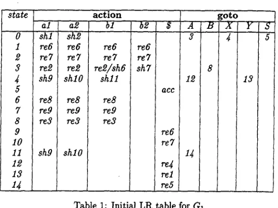
From the CFG given in Figure 4, we can generate an LR table, Table 1, in Step 1 using the conven- tional LR table generation algorithm.

Table 2 is the resultant LR table at the completion of Step 2 and Step 3, produced based on Table 1. Actions numbered (2) and (3) in Table 2 are those which are removed by Step 2 and Step 3, respectively.

In state 1 with a lookahead symbol bl, re6 is carried out after executing action shl in state 0, pushing al onto the stack. Note that al and bl are now consecutive, in this order. However, the probabilistic connection matrix (see Figure 5) does not allow such a sequence of terminal symbols, since PConnect( al , bl ) = O. Therefore, the action re6 in state 1 with lookahead bl is removed from Ta- ble 1 in Step 2, and thus marked as (2) in Table 2.

For this same reason, the other re6s in state 1 with lookahead symbols al and a$ are also removed from Table 1.

On the other hand, in the case of re6 in state 1 with lookahead symbol b$, as al can be followed by b2 (PConnect(al, b~) ~ 0), action re6 cannot be removed. The remaining actions marked as (2} in Table 2 should be self-evident to readers.

Next, we would like to consider the reason why action sh9 in state 4 with lookahead al is removed from Table 1. In state 9, re6 with lookahead symbol $ has already been removed in Step 2, and there is no succeeding action for shg. Therefore, action sh9 in state 3 is removed in Step 3, and hence marked as(3).

Let us consider action re3 in state 8 with lookahead al. After this action is carried out, the G L R parser goes to state 4 after pushing X onto the stack. However, sh9 in state 4 with lookahead al has al- ready been removed, and there is no succeeding action for re3. As a result, re3 in state 8 with lookahead symbol al is removed in Step 3. Similarly, re9 in state 7 with lookahead symbol al is also removed in Step 3. In this way, the removal of actions prop- agates to other removals. This chain of removals is called Constraint Propagation, and occurs in Step 3. Actions removed in Step 3 are marked as (3) in Table 2.

Careful readers will notice that there is now no action in state 9 and that it is possible to delete this state in Step 4. Table 3 shows the LR table after Step 4.

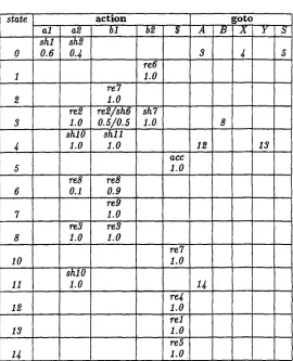
As a final step, we would like to assign big-ram constraints to each action in Table 3. Let us consider the two tess in state 6, reached after executing sh6 in state 4 by pushing a lookahead of bl onto the stack. In state 6, P is calculated at Step 5 as shown below:

P = PConnect(bl,a2) + P C o n n e c t ( b l , b l ) = 0 . 1 + 0 . 9

= 1

We can assign the following probabilities p to each re8 in state 6 by way of Step 5:

PCon,~ect(bl,ae) for re8 with

p×n = ~ = 0.I lookahead a2

P = PConnect(bl,bl ) for re8 with

P×n = ~ = 0.9 lookahead bl

After assigning a probability to each action in the LR table at Step 5, there remain actions without probabilities. For example, the two conflict actions (re2/sh6) in state 3 with lookahead bl are not assigned a probability. Therefore, each of these actions is assigned the same probability, 0.5, in Step 7. A probability of 1 is assigned to remaining actions, since there is no conflict among them.

Table 4 shows the final results of applying Algo- rithm 1 to G, and M,.

II

(5)

II

state

0 1 2 3

4

5 6 7 8 9 10 11 12 13

14.

al shl re6 re7 re2 sh9

re8 re9 re3

sh9 a2 she re6 re7 re2 shlO

re8 re9 re3

shlO

a c t i o n bl

re6 re7 ree/sh6

sh11

re8 re9 re3

b2

re6 re7 sh7

i

$ A

3

12 a c e

re6 re7

~4

re1 re5

Table 1: Initial LR table for G1

goto

B X

4

8

Y

13 S 5

state

0 1 2 3

4

5 6 7 8 9 10 11 12 13 14.

al shl re6(2)

reT(e)

tee(3) shg(3)

re8(2) reg(3) re3(3)

shg(3) a2 she re6(2) re7(2) re2 shlO

re8 re9(2)

re3

shlO

a c t i o n bl

re7 re2/sh6

sh11

re8 re9 re3

b2 $ A

3 re6

re7(2) sh7

12 a c e

re7 14

re4

re1 re5

Table 2: LR table after Steps 2 and 3

goto

B X Y S

4

5

8

13

[image:5.612.165.440.80.286.2]

(6)

state

0 1 2 3

4

5 6 7 8 10 11 12 i3

14

al

sh'l

a2 sh2

re2 shlO

re8

re3

sh10

action

bl

re7 re2/sh6

s h l l

re8 re9 re3

b2

re6

sh7

$ A

3

12 acc

re7

14 re4

re1 re5

Table 3: LR table after Step 4

goto

B X

4

Y

13 S 5

state

0

1

.2

3

4

5

6

7

8

10

11

12

13

14

al shl 0.6

a2 sh2

0.4

re2 1.0 shlO

1.0

re8 0.1

re3 1.0

shlO 1.0

action

bl b2 $

re6 1.0 re7 1.0

re2/sh6 Sh 7

0.5/0.5

1.o

s h l l 1.0

re8 0.9 re9 1.0 re3 1.0

acc 1.0

re7 1.0

re4

1.0 tel 1.0 re5 1 . 0

A

3

goto

B X Y

8

12 13

14

Table 4: The Bigram LR table constructed by Algorithm 1

II

I!

II

k

[image:6.612.177.449.73.256.2] [image:6.612.177.447.302.635.2]

(7)

4.2 Comparison of Language Models

Using the bigram LR table as shown in Table 4, the probability P1 of the string "a2 bl ag' is calculated

a s :

P1 = P(a2 bl ae)

T

= E P(Tree0

i = l

= P(O, ae, she) x P(2, bl,re7)

xP(3, bI, re._~2) x P(4, bl, sh11)

x P ( l l , a2, shlO) x P(10, $, re7)

xP(14, $, re5) x P(13, $, re1 )

×P(5, $, acc)

+ P(O, a2, she) x P(2, bl, re7)

xP(3, bl, sh_66) x P(6, a2, reS)

xP(8, ae, re3) x P(4, ae, shlO)

xP(10, $, re7) x P(12, $, re4 ) xP(13,$, re1) x P(5, $, acc)

= 0.4 x 1.0 x 0.5 x 1.0 x 1.0

x 1.0 x 1.0 x 1.0 x 1.0

+ 0.4 x 1.0 x 0.5 x 0.1 x 1.0 x 1.0 x 1.0 x 1.0 x 1.0 x 1.0 = 0.2 + 0.02

= 0.22

where P(Treei) means the probability of the i- th parsing tree generated by the GLR parser and

P ( S , L , A ) means the probability of an action A in state S with Iookahead L.

On the other hand, using only bigram constraints, the probability P2 of the string "ae b1 a,~' is calculated as:

P2 = P(a2 bl a2)

= P(ael#) × P(bllae) x P(aelbl) × P($1ae)

= x0.3 x0.1 x 0 . 7 = 0.0084

The reason why P1 > P2 can be explained as follows. Consider the beginning symbol a2 of a sentence. In the case of the bigram model, a2 can only be followed by either of the two symbols bl and $

(see Figure 5). However, consulting the bigram LR table reveals that in state 0 with lookahead ae, she

is carried out, entering state 2. State 2 has only one action re7 with lookahead symbol bl. In other words, in state 2, $ is not predicted as a succeeding symbol of al. The exclusion of an ungrammatical prediction in $ makes P1 larger than P2.

Perplexity is a measure of the complexity of a language model. The larger the probability of the language model, the smaller the perplexity of the language model. The above result (P1 > P2) indicates

I Language model I Perplexity I

Bigram 6.50

BigraJfi LR table 5.99

Trigram 4.92

Table 5: Perplexity of language models

that the bigram LR table model gives smaller perplexity than the bigram model. In the next section, we will demonstrate this fact.

5 Evaluation of Perplexity

Perplexity is a measure of the constraint imposed by the language model. Test-set perplexity (Jelinek, 1990) is commonly used to measure the perplexity of a language model from a test-set. Test-set perplexity

for a language model L is simply the geometric mean of probabilities defined by:

where

Q(L) = 2//(L)

1 M

S ( L ) =

logP(S,)

i = l

Here N is the number of terminal symbols in the test set, M is the number of test sentences and P(S,) is the probability of generating i-th test sentence Si.

In the case of the bigram model, P~i(Si) is:

Pb~(&) = P ( z l , z e , . . . , z . )

= P ( z I I # ) P ( z e I z l ) . . . P ( x ~ I z . _ I ) P ( $ 1 . . )

And in the case of the trigram model, P~(Si) is: Pt~i(S~) = P ( x l , z e , . . . , z , )

= P(xll#)P(xel#,xl)...

P ( x . I x . - 2 , x.-1)P($lx.-a, x.)

Table 5 shows the test-set perplexity of pretermi- rials for each language model. Here the preterminal bigram models were trained on a corpus with 20663 sentences, containing 230927 preterminals. The test- set consists of 1320 sentences, which contain 13311 preterminals. The CFG used is a phrase context- free grammar used in speech recognition tasks, and the number of rules and preterminals is 777 and 407, respectively.

As is evident from Table 5, the use of a bigram LR table decreases the test-set perplexity from 6.50 to 5.99. Note that in this experiment, we used the LALR table generation algorithm 2 to construct the bigram LR table. Despite the disadvantages of

2In the case of LALR tables, the sum of the proba- bihties of all the possible parsing trees generated by a given CFG may be less than 1 (Inui et al., 1997).

[image:7.612.307.446.99.148.2]

(8)

LALR tables, the bigram LR table has better performance than the simple bigram language model, showing the effectiveness of a bigram LR table.

On the other hand, the perplexity of the trigram language model is smaller than that of the bigram LR table. However, with regard to data sparseness, the bigram LR table is better than the trigram language model because bigram constraints are more easily acquired from a given corpus than trigram constraints.

Although the experiment described above is concerned with natural language processing, our method is also applicable to speech recognition.

6 C o n c l u s i o n s

In this paper, we described a method to construct a bigram LR table, and then discussed the advantage of our method, comparing our method to the bigram and trigram language models. The principle advantage over the bigram language model is that, in using a bigram LR table, we can combine both local probabilistic connection constraints (bigram constraints) and global constraints (CFG).

Our method is applicable not only to natural language processing but also speech recognition. We are currently testing our method using a large- sized grammar containing dictionary rules for speech recognition.

Su et al. (Suet al., 1991) and Chiang et al. (Chi- ang et al., 1995) have proposed a very interesting corpus-based natural language processing method that takes account not only of lexical, syntactic, and semantic scores concurrently, but also context- sensitivity in the language model. However, their method seems to suffer from difficulty in acquiring probabilities from a given corpus.

Wright (Wright, 1990) developed a method of dis- tributing the probability of each PCFG rule to each action in an LR table. However, this method only calculates syntactic scores of parsing trees based on a context-free framework.

Briscoe and Carroll (Briscoe and Carroll., 1993) attempt to incorporate probabilities into an LR table. They insist that the resultant probabilistic LR table can include probabilities with context- sensitivity. Inui et. al. (Inni et al., 1997)reported that the resultant probabilistic LR table has a defect in terms of the process used to normalize probabilities associated with each action in the LR table.

• Finally, we would like to mention that Klavans and Resnik (Klavaus and Resnik, 1996) have ad- vocated a similar approach to ours which combines symbolic and statistical constraints, CFG and bigram constraints.

A c k n o w l e d g e m e n t s

We would like to thank Mr. Toshiyuki Takezawa and Mr. Junji Etoh for providing us the dialog corpus

and the grammar for our experiments. We would also like to thank Mr. Timothy Baldwin for his help in writing this paper.

R e f e r e n c e s

A.V. Aho, S. Ravi, and J.D. UUman. 1986.

Com-

pilers: Principle, Techniques, and Tools.

Addison

Wesley.

T. Briscoe and J. Carroll. 1993. Generalized probabilistic LR parsing of natural language (corpora) with unification-based grammars.

Computational

Linguistics,

19(1):25-59.

T.H. Chiang, Y.C. Lin, and K.Y. Su. 1995. Robust learning, smoothing, and parameter tying on syntactic ambiguity resolution.

Computational Lin-

guistics,

21(3):321-349.

A. Franz. 1996.

Automatic Ambiguity Resolution in

Natural Language Processing.

Springer.

T. Fujisaki, F. Jelinek, J. Cocke, E. Black, and T. Nishino. 1991. A probabilistic parsing method for sentence disambiguation. In M. Tomita, editor,

Current Issues in Parsing Technologies,

pages 139-152. Kluwer Academic Publishers.

K. Inui, V. Sornlertlamvanich, H. Tanaka, and T. Tokunaga. 1997. A new formalization of probabilistic GLR parsing. In

International Workshop

on Parsing Technologies.

F. Jelinek. 1990. Self-organized language mod- eling for speech recognition. In A. Waibel and K.F. Lee, editors,

Readings in Speech Recognition,

pages 450-506. Morgan Kauhnann.

J.L. Klavans and P. Resnik. 1996.

The Balanc-

ing Act: Combining Symbolic and S~atistial Ap-

proaches to Language.

The MIT Press.

D.E. Knuth. 1965. On the translation of languages left to right.

Information and Control,

8(6):607- 639.

K.F. Lee. 1989.

Automatic Speech Recognition:

The Development of the SPHINX System.

Kluwer

Academic Publishers.

K.Y. Su, J.N. Wang, M.H. Su, and J.S. Chang. 1991. GLR parsing with scoring. In M. Tomita, editor,

Generalized LR Parsing.

Kluwer Academic Pub-

fishers.

H. Tanaka, H. Li, and T. Tokunaga. 1994. Incor- poration of phoneme-context-dependence into LR table through constraints propagation method. In

Workshop on Integration of Natural Language and

Speech Processing,

pages 15-22.

H. Tanaka, T. Takezawa, and J. Etoh. 1997. Japanese grammar for speech recognition considering the MSLR method. In

Information Process-

ing Society of Japan, SIG-SLP-15,

pages 145-150.

(9)

l

/

i

I

/

I

M. Tomita. 1986. Efficient Parsing for Natural Lan- guage: A Fast Algorithm for Practical Systems.

Kluwer' Academic Publishers.

J.I-I. Wright. 1990. LR parsing of probabilistic grammars with input uncertainty for speech recognition. Computer Speech and Language, 4(4):297- 323.