Semantic Matching of Documents from
Heterogeneous Collections:
A Simple and Transparent Method for Practical Applications
Mark-Christoph M¨uller
Heidelberg Institute for Theoretical Studies gGmbH Heidelberg, Germany
mark-christoph.mueller@h-its.org
Abstract
We present a very simple, unsupervised method for the pairwise matching of documents from het-erogeneous collections. We demonstrate our method with the Concept-Project matching task, which is a binary classification task involving pairs of documents from heterogeneous collections. Although our method only employs standard resources without any domain- or task-specific modifications, it clearly outperforms the more complex system of the original authors. In addition, our method is
transparent, because it provides explicit information about how a similarity score was computed, andefficient, because it is based on the aggregation of (pre-computable) word-level similarities.
1
Introduction
We present a simple and efficient unsupervised method for pairwise matching of documents from
het-erogeneouscollections. Following Gong et al. (2018), we consider two document collections heteroge-neous if their documents differ systematically with respect to vocabulary and / or level of abstraction. With thesedefiningdifferences, there often also comes a difference in length, which, however, by itself
does not make document collections heterogeneous. Examples include collections in whichexpert
an-swers are mapped to non-expertquestions (e.g.InsuranceQAby Feng et al. (2015)), but also so-called
communityQA collections (Blooma and Kurian (2011)), where the lexical mismatch between Q and A documents is often less pronounced than the length difference.
Like many other approaches, the proposed method is based on word embeddings as universal meaning representations, and on vector cosine as the similarity metric. However, instead of computing pairs of document representations and measuring their similarity, our method assesses the document-pair simi-larity on the basis of selected pairwise word similarities. This has the following advantages, which make
our method a viable candidate for practical, real-world applications: efficiency, because pairwise word
similarities can be efficiently (pre-)computed and cached, andtransparency, because the selected words
from each document are available as evidence for what the similarity computation was based on.
We demonstrate our method with the Concept-Project matching task (Gong et al. (2018)), which is
described in the next section.
2
Task, Data Set, and Original Approach
The Concept-Project matchingtask is a binary classification task where each instance is a pair of
het-erogeneous documents: oneconcept, which is a short science curriculum item from NGSS1, and one
project, which is a much longer science project description for school children from ScienceBuddies2.
1https://www.nextgenscience.org
CONCEPT LABEL: ecosystems: - ls2.a: interdependent relationships in ecosystems
CONCEPT DESCRIPTION:Ecosystems have carrying capacities , which are limits to the numbers of organisms and populations they can support . These limits result from such factors as the availability of living and nonliving resources and from such challenges such as predation , competition , and disease . Organisms would have the capacity to produce populations of great size were it not for the fact that environments and resources are finite . This fundamental tension affects the abundance ( number of individuals ) of species in any given ecosystem .
PROJECT LABEL: Primary Productivity and Plankton
PROJECT DESCRIPTION:Have you seen plankton? I am not talking about the evil villain trying to steal the Krabby Patty recipe from Mr. Krab. I am talking about plankton that live in the ocean. In this experiment you can learn how to collect your own plankton samples and see the wonderful diversity in shape and form of planktonic organisms. The oceans contain both the earth’s largest and smallest organisms. Interestingly they share a delicate relationship linked together by what they eat. The largest of the ocean’s inhabitants, the Blue Whale, eats very small plankton, which themselves eat even smaller phytoplankton. All of the linkages between predators, grazers, and primary producers in the ocean make up an enormously complicated food web.The base of this food web depends upon phytoplankton, very small photosynthetic organisms which can make their own energy by using energy from the sun. These phytoplankton provide the primary source of the essential nutrients that cycle through our ocean’s many food webs. This is called primary productivity, and it is a very good way of measuring the health and abundance of our fisheries.There are many different kinds of phytoplankton in our oceans. [...] One way to study plankton is to collect the plankton using a plankton net to collect samples of macroscopic and microscopic plankton organisms. The net is cast out into the water or trolled behind a boat for a given distance then retrieved. Upon retrieving the net, the contents of the collecting bottle can be removed and the captured plankton can be observed with a microscope. The plankton net will collect both phytoplankton (photosynthetic plankton) and zooplankton (non-photosynthetic plankton and larvae) for observation.In this experiment you will make your own plankton net and use it to collect samples of plankton from different marine or aquatic locations in your local area. You can observe both the abundance (total number of organisms) and diversity (number of different kinds of organisms) of planktonic forms to make conclusions about the productivity and health of each location. In this experiment you will make a plankton net to collect samples of plankton from different locations as an indicator of primary productivity. You can also count the number of phytoplankton (which appear green or brown) compared to zooplankton (which are mostly marine larval forms) and compare. Do the numbers balance, or is there more of one type than the other? What effect do you think this has on productivity cycles? Food chains are very complex. Find out what types of predators and grazers you have in your area. You can find this information from a field guide or from your local Department of Fish and Game. Can you use this information to construct a food web for your local area? Some blooms of phytoplankton can be harmful and create an anoxic environment that can suffocate the ecosystem and leave a ”Dead Zone” behind. Did you find an excess of brown algae or diatoms? These can be indicators of a harmful algal bloom. Re-visit this location over several weeks to report on an increase or decrease of these types of phytoplankton. Do you think that a harmful algal bloom could be forming in your area? For an experiment that studies the relationship between water quality and algal bloom events, see the Science Buddies project Harmful Algal Blooms in the Chesapeake Bay.
Figure 1: C-P Pair (Instance261of the original data set.)
The publicly available data set3 contains 510labelled pairs4 involving C = 75unique concepts and
P = 230unique projects. A pair is annotated as1if the project matches the concept (57%), and as0
otherwise (43%). The annotation was done by undergrad engineering students. Gong et al. (2018) do
not provide any specification, or annotation guidelines, of the semantics of the ’matches’ relation to be annotated. Instead, they create gold standard annotations based on a majority vote of three manual anno-tations. Figure 1 provides an example of a matching C-P pair. The concept labels can be very specific, potentially introducing vocabulary that is not present in the actual concept descriptions. The extent to which this information is used by Gong et al. (2018) is not entirely clear, so we experiment with several setups (cf. Section 4).
2.1 Gong et al. (2018)’s Approach
The approach by Gong et al. (2018) is based on the idea that the longer document in the pair is reduced
to a set of topics which capture the essence of the document in a way that eliminates the effect of a
potential length difference. In order to overcome the vocabulary mismatch, these topics are not based on words and their distributions (as in LSI (Deerwester et al. (1990)) or LDA (Blei et al. (2003))), but on word embedding vectors. Then, basically, matching is done by measuring the cosine similarity between the topic vectors and the short document words. Gong et al. (2018) motivate their approach mainly with the length mismatch argument, which they claim makes approaches relying on document representations (incl. vector averaging) unsuitable. Accordingly, they use Doc2Vec (Le and Mikolov (2014)) as one of their baselines, and show that its performance is inferior to their method. They do not, however, provide a much simpler averaging-based baseline. As a second baseline, they use Word Mover’s Distance (Kusner et al. (2015)), which is based on word-level distances, rather than distance of global document representations, but which also fails to be competitive with their topic-based method. Gong et al. (2018) use two different sets of word embeddings: One (topic wiki) was trained on a full English Wikipedia dump, the other (wiki science) on a smaller subset of the former dump which only contained science articles.
3
Our Method
We develop our method as a simple alternative to that of Gong et al. (2018). We aim at comparable or better classification performance, but with a simpler model. Also, we design the method in such a way that it provides human-interpretable results in an efficient way. One common way to compute
3
the similarity of two documents (i.e. word sequences)candpis to average over the word embeddings for each sequence first, and to compute the cosine similarity between the two averages afterwards. In the first step, weighting can be applied by multiplying a vector with the TF, IDF, or TF*IDF score of
its pertaining word. We implement this standard measure (AVG COS SIM) as a baseline for both our
method and for the method by Gong et al. (2018). It yields a single scalar similarity score. The core idea of our alternative method is to turn the above process upside down, by computing the cosine similarity ofselectedpairs of words fromcandpfirst, and to average over the similarity scores afterwards (cf. also
Section 6). More precisely, we implement a measureTOP n COS SIM AVGas the average of then
highest pairwise cosine similarities of the ntop-ranking words in candp. Ranking, again, is done by
TF, IDF, and TF*IDF. For each ranking, we take the top-rankingnwords fromcandp, computen×n
similarities, rank by decreasing similarity, and average over the topnsimilarities. This measure yields both a scalar similarity score and a list of< cx, py, sim >tuples, which represent the qualitative aspects
ofcandpon which the similarity score is based.
4
Experiments
Setup All experiments are based on off-the-shelf word-level resources: We employ WOMBAT (M¨uller
and Strube (2018)) for easy access to the 840B GloVe (Pennington et al. (2014)) and the GoogleNews5
Word2Vec (Mikolov et al. (2013)) embeddings. These embedding resources, while slightly outdated, are still widely used. However, they cannot handle out-of-vocabulary tokens due to their fixed, word-level
lexicon. Therefore, we also use a pretrained English fastText model6 (Bojanowski et al. (2017); Grave
et al. (2018)), which also includes subword information. IDF weights for approx.12mio. different words
were obtained from the English Wikipedia dump provided by the Polyglot project (Al-Rfou et al. (2013)). All resources are case-sensitive, i.e. they might contain different entries for words that only differ in case (cf. Section 5).
We run experiments in different setups, varying both the input representation (GloVe vs. Google vs.
fastText embeddings,±TF-weighting, and±IDF-weighting) for concepts and projects, and the extent to
which concept descriptions are used: For the latter,Labelmeans only the conceptlabel(first and second
row in the example),Descriptionmeans only the textualdescriptionof the concept, andBothmeans the
concatenation ofLabelandDescription. For the projects, we always use both label and description. For
the project descriptions, we extract only the last column of the original file (CONTENT), and remove user comments and some boiler-plate. Each instance in the resulting data set is a tuple of< c, p, label >,
wherecandpare bags of words, with case preserved and function words7removed, andlabelis either0
or1.
Parameter Tuning Our method is unsupervised, but we need to define a threshold parameter which
controls the minimum similarity that a concept and a project description should have in order to be
considered a match. Also, the TOP n COS SIM AVG measure has a parameternwhich controls how
many ranked words are used from candp, and how many similarity scores are averaged to create the
final score. Parameter tuning experiments were performed on a random subset of20%of our data set
(54% positive). Note that Gong et al. (2018) used only 10%of their 537instances data set as tuning
data. The tuning data results of the best-performing parameter values for each setup can be found in
Tables 1 and 2. The top F scores per type of concept input (Label, Description, Both) are given inbold.
For AVG COS SIM and TOP n COS SIM AVG, we determined the threshold values (T) on the tuning
data by doing a simple.005step search over the range from0.3to1.0. For TOP n COS SIM AVG, we
additionally varied the value ofnin steps of2from2to30.
5https://code.google.com/archive/p/word2vec/
6https://dl.fbaipublicfiles.com/fasttext/vectors-crawl/cc.en.300.bin.gz
7
Results The toptuning datascores for AVG COS SIM (Table 1) show that the Google embeddings
with TF*IDF weighting yield the top F score for all three concept input types (.881-.945). Somewhat
expectedly, the best overall F score (.945) is produced in the setting Both, which provides the most
information. Actually, this is true for all four weighting schemes for both GloVe and Google, while fastText consistently yields its top F scores (.840-.911) in theLabelsetting, which provides the least information. Generally, the level of performance of the simple baseline measure AVG COS SIM on this data set is rather striking.
Concept Input→ Label Description Both Embeddings TF IDF T P R F T P R F T P R F
GloVe
- - .635 .750 .818 .783 .720 .754 .891 .817 .735 .765 .945 .846
+ - .640 .891 .745 .812 .700 .831 .891 .860 .690 .813 .945 .874
- + .600 .738 .873 .800 .670 .746 .909 .820 .755 .865 .818 .841
+ + .605 .904 .855 .879 .665 .857 .873 .865 .715 .923 .873 .897
- - .440 .813 .945 .874 .515 .701 .982 .818 .635 .920 .836 .876
+ - .445 .943 .909 .926 .540 .873 .873 .873 .565 .927 .927 .927
- + .435 .839 .945 .889 .520 .732 .945 .825 .590 .877 .909 .893
+ + .430 .943 .909 .926 .530 .889 .873 .881 .545 .945 .945 .945
fastText
- - .440 .781 .909 .840 .555 .708 .927 .803 .615 .778 .891 .831
+ - .435 .850 .927 .887 .520 .781 .909 .840 .530 .803 .964 .876
- + .435 .850 .927 .887 .525 .722 .945 .819 .600 .820 .909 .862
[image:4.595.144.453.177.312.2]+ + .420 .895 .927 .911 .505 .803 .891 .845 .520 .833 .909 .870
Table 1: Tuning Data ResultsAVG COS SIM. Top F per Concept Input Type inBold.
For TOP n COS SIM AVG, thetuning dataresults (Table 2) are somewhat more varied: First, there
is no single best performing set of embeddings: Google yields the best F score for the Label setting
(.953), while GloVe (though only barely) leads in theDescriptionsetting (.912). This time, it is fastText
which produces the best F score in theBothsetting, which is also the best overalltuning dataF score
for TOP n COS SIM AVG (.954). While the difference to the Google result forLabelis only minimal,
it is striking that the best overall score is again produced using the ’richest’ setting, i.e. the one involving both TF and IDF weighting and the most informative input.
Concept Input→ Label Description Both Embeddings TF IDF T/n P R F T/n P R F T/n P R F
GloVe
+ - .365/6 .797 .927 .857 .690/14.915 .782 .843 .675/16.836 .927 .879
- + .300/30 .929 .236 .377 .300/30.806 .455 .581 .300/30.778 .636 .700
+ + .330/6 .879 .927 .903 .345/6 .881 .945 .912 .345/6 .895 .927 .911
+ - .345/22 .981 .927 .953 .480/16.895 .927 .911 .520/16.912 .945 .929
- + .300/30 1.00.345 .514 .300/8 1.00 .345 .514 .300/30 1.00 .600 .750
+ + .300/10 1.00.509 .675 .300/14.972 .636 .769 .350/22 1.00 .836 .911
fastText
+ - .415/22 .980 .873 .923 .525/14.887 .855 .870 .535/20.869 .964 .914
- + .350/24 1.00.309 .472 .300/30 1.00 .382 .553 .300/28 1.00 .673 .804
[image:4.595.125.471.450.556.2]+ + .300/20 1.00.800 .889 .300/10.953 .745 .837 .310/14.963 .945 .954
Table 2: Tuning Data ResultsTOP n COS SIM AVG. Top F per Concept Input Type inBold.
We then selected the best performing parameter settings for every concept input and ran experiments on
the held-out test data. Since the original data split used by Gong et al. (2018) is unknown, we cannot
exactly replicate their settings, but we also perform ten runs using randomly selected 10%of our408
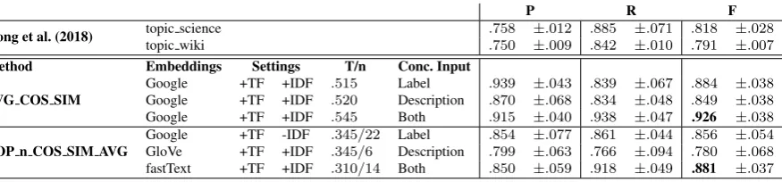
instances test data set, and report average P, R, F, and standard deviation. The results can be found in Table 3. For comparison, the two top rows provide the best results of Gong et al. (2018).
The first interesting finding is that the AVG COS SIM measure again performs very well: In all three settings, it beats both the system based on general-purpose embeddings (topic wiki) and the one that is adapted to the science domain (topic science), with again theBothsetting yielding the best overall result
(.926). Note that ourBothsetting is probably the one most similar to the concept input used by Gong
P R F
Gong et al. (2018) topic science .758 ±.012 .885 ±.071 .818 ±.028 topic wiki .750 ±.009 .842 ±.010 .791 ±.007
Method Embeddings Settings T/n Conc. Input
AVG COS SIM
Google +TF +IDF .515 Label .939 ±.043 .839 ±.067 .884 ±.038 Google +TF +IDF .520 Description .870 ±.068 .834 ±.048 .849 ±.038 Google +TF +IDF .545 Both .915 ±.040 .938 ±.047 .926 ±.038
TOP n COS SIM AVG
[image:5.595.85.523.69.171.2]Google +TF -IDF .345/22 Label .854 ±.077 .861 ±.044 .856 ±.054 GloVe +TF +IDF .345/6 Description .799 ±.063 .766 ±.094 .780 ±.068 fastText +TF +IDF .310/14 Both .850 ±.059 .918 ±.049 .881 ±.037
Table 3: Test Data Results
three settings. It only fails in the setting using only theDescriptioninput.8 This is the more important as we exclusively employ off-the-shelf, general-purpose embeddings, while Gong et al. (2018) reach their best results with a much more sophisticated system and with embeddings that were custom-trained for the science domain. Thus, while the performance of our proposed TOP n COS SIM AVG method is superior to the approach by Gong et al. (2018), it is itself outperformed by the ’baseline’ AVG COS SIM method with appropriate weighting. However, apart from raw classification performance, our method also aims at providing human-interpretable information on how a classification was done. In the next section, we perform a detail analysis on a selected setup.
5
Detail Analysis
The similarity-labelled word pairs from concept and project description which are selected during clas-sification with the TOP n COS SIM AVG measure provide a way to qualitatively evaluate the basis on which each similarity score was computed. We see this as an advantage over average-based comparison (like AVG COS SIM), since it provides a means to check the plausibility of the decision. Here, we are
mainly interested in the overall best result, so we perform a detail analysis on the best-performingBoth
setting only (fastText, TF*IDF weighting,T =.310,n= 14). Since theConcept-Project matchingtask
is a binary classification task, its performance can be qualitatively analysed by providing examples for instances that were classified correctly (True Positive (TP) and True Negative (TN)) or incorrectly (False Positive (FP) and False Negative (FN)).
Table 5 shows the concept and project words from selected instances (one TP, FP, TN, and FN case each) of the tuning data set. Concept and project words are ordered alphabetically, with concept words appearing more than once being grouped together. According to the selected setting, the number of word
pairs is n = 14. The bottom line in each column provides the average similarity score as computed
by the TOP n COS SIM AVG measure. This value is compared against the threshold T = .310. The
similarity is higher than T in the TP and FP cases, and lower otherwise. Without going into too much
detail, it can be seen that the selected words provide a reasonable idea of the gist of the two documents. Another observation relates to the effect of using unstemmed, case-sensitive documents as input: the
top-ranking words often contain inflectional variants (e.g.enzyme andenzymes, levelandlevels in the
example), and words differing in case only can also be found. Currently, these are treated as distinct (though semantically similar) words, mainly out of compatibility with the pretrained GloVe and Google embeddings. However, since our method puts a lot of emphasis on individual words, in particular those
coming from the shorter of the two documents (the concept), results might be improved by somehow
merging these words (and their respective embedding vectors) (see Section 7).
6
Related Work
While in this paper we apply our method to the Concept-Project matching task only, the underlying
task of matching text sequences to each other is much more general. Many existing approaches follow
8
TP (.447> .310) FP (.367> .310) TN (.195< .310) FN (.278< .310)
Concept Project
Sim Concept Project Sim Concept Project Sim Concept Project Sim
Word Word Word Word Word Word Word Word
cells enzymes .438 co-evolution dynamic .299 energy allergy .147 area water .277
cells genes .427 continual dynamic .296 energy juice .296 climate water .269
molecules DNA .394 delicate detail .306 energy leavening .186 earth copper .254
molecules enzyme .445 delicate dynamic .326 energy substitutes .177 earth metal .277
molecules enzymes .533 delicate texture .379 surface average .212 earth metals .349
molecules gene .369 dynamic dynamic 1.00 surface baking .216 earth water .326
molecules genes .471 dynamic image .259 surface egg .178 extent concentration .266
multiple different .550 dynamic range .377 surface leavening .158 range concentration .255
organisms enzyme .385 dynamic texture .310 surface thickening .246 range ppm .237
organisms enzymes .512 surface level .323 transfer baking .174 systems metals .243
organisms genes .495 surface texture .383 transfer substitute .192 systems solution .275
organs enzymes .372 surface tiles .321 transfer substitutes .157 typical heavy .299
tissues enzymes .448 systems dynamic .272 warms baking .176 weather heavy .248
tissues genes .414 systems levels .286 warms thickening .214 weather water .308
[image:6.595.76.514.69.270.2]Avg. Sim .447 Avg. Sim .367 Avg. Sim .195 Avg. Sim .278
Table 4:TOP n COS SIM AVGDetail Results of Best-performing fastText Model onBoth.
the so-called compare-aggregate framework (Wang and Jiang (2017)). As the name suggests, these
approaches collect the results of element-wise matchings (comparisons) first, and create the final result
by aggregating these results later. Our method can be seen as a variant ofcompare-aggregatewhich is
characterized by extremely simple methods for comparison (cosine vector similarity) and aggregation (averaging). Other approaches, like He and Lin (2016) and Wang and Jiang (2017), employ much more elaborated supervised neural networks methods. Also, on a simpler level, the idea of averaging similarity scores (rather than scoring averaged representations) is not new: Camacho-Collados and Navigli (2016)
use the average of pairwise word similarities to compute theircompactness score.
7
Conclusion and Future Work
We presented a simple method for semantic matching of documents from heterogeneous collections as a
solution to theConcept-Project matchingtask by Gong et al. (2018). Although much simpler, our method
clearly outperformed the original system in most input settings. Another result is that, contrary to the claim made by Gong et al. (2018), the standard averaging approach does indeed work very well even for heterogeneous document collections, if appropriate weighting is applied. Due to its simplicity, we believe that our method can also be applied to other text matching tasks, including more ’standard’ ones which do
not necessarily involveheterogeneousdocument collections. This seems desirable because our method
offers additional transparency by providing not only a similarity score, but also the subset of words on which the similarity score is based. Future work includes detailed error analysis, and exploration of methods to combine complementary information about (grammatically or orthographically) related words from word embedding resources. Also, we are currently experimenting with a pretrained ELMo (Peters et al. (2018)) model as another word embedding resource. ELMo takes word embeddings a step
further by dynamically creatingcontextualizedvectors from input word sequences (normally sentences).
Our initial experiments have been promising, but since ELMo tends to yielddifferent, context-dependent
vectors for thesameword in thesamedocument, ways have still to be found to combine them into single,
document-wide vectors, without (fully) sacrificing their context-awareness.
The code used in this paper is available athttps://github.com/nlpAThits/TopNCosSimAvg.
References
Al-Rfou, R., B. Perozzi, and S. Skiena (2013, August). Polyglot: Distributed word representations for
multilingual nlp. InProceedings of the Seventeenth Conference on Computational Natural Language
Learning, Sofia, Bulgaria, pp. 183–192. Association for Computational Linguistics.
Blei, D. M., A. Y. Ng, and M. I. Jordan (2003). Latent dirichlet allocation. Journal of Machine Learning
Research 3, 993–1022.
Blooma, M. J. and J. C. Kurian (2011). Research issues in community based question answering. In P. B.
Seddon and S. Gregor (Eds.),Pacific Asia Conference on Information Systems, PACIS 2011:
Qual-ity Research in Pacific Asia, Brisbane, Queensland, Australia, 7-11 July 2011, pp. 29. Queensland University of Technology.
Bojanowski, P., E. Grave, A. Joulin, and T. Mikolov (2017). Enriching word vectors with subword
information. TACL 5, 135–146.
Camacho-Collados, J. and R. Navigli (2016). Find the word that does not belong: A framework for an
intrinsic evaluation of word vector representations. InProceedings of the 1st Workshop on Evaluating
Vector-Space Representations for NLP, RepEval@ACL 2016, Berlin, Germany, August 2016, pp. 43– 50. Association for Computational Linguistics.
Deerwester, S. C., S. T. Dumais, T. K. Landauer, G. W. Furnas, and R. A. Harshman (1990). Indexing
by latent semantic analysis. JASIS 41(6), 391–407.
Feng, M., B. Xiang, M. R. Glass, L. Wang, and B. Zhou (2015). Applying deep learning to answer
selection: A study and an open task. In2015 IEEE Workshop on Automatic Speech Recognition and
Understanding, ASRU 2015, Scottsdale, AZ, USA, December 13-17, 2015, pp. 813–820. IEEE.
Gong, H., T. Sakakini, S. Bhat, and J. Xiong (2018). Document similarity for texts of varying lengths
via hidden topics. InProceedings of the 56th Annual Meeting of the Association for Computational
Linguistics (Volume 1: Long Papers), pp. 2341–2351. Association for Computational Linguistics.
Grave, E., P. Bojanowski, P. Gupta, A. Joulin, and T. Mikolov (2018). Learning word vectors for 157 languages. In N. Calzolari, K. Choukri, C. Cieri, T. Declerck, S. Goggi, K. Hasida, H. Isahara, B.
Mae-gaard, J. Mariani, H. Mazo, A. Moreno, J. Odijk, S. Piperidis, and T. Tokunaga (Eds.),Proceedings of
the Eleventh International Conference on Language Resources and Evaluation, LREC 2018, Miyazaki, Japan, May 7-12, 2018.European Language Resources Association (ELRA).
He, H. and J. J. Lin (2016). Pairwise word interaction modeling with deep neural networks for semantic
similarity measurement. In K. Knight, A. Nenkova, and O. Rambow (Eds.),NAACL HLT 2016, The
2016 Conference of the North American Chapter of the Association for Computational Linguistics: Human Language Technologies, San Diego California, USA, June 12-17, 2016, pp. 937–948. The Association for Computational Linguistics.
Kusner, M. J., Y. Sun, N. I. Kolkin, and K. Q. Weinberger (2015). From word embeddings to document
distances. In F. R. Bach and D. M. Blei (Eds.),Proceedings of the 32nd International Conference on
Machine Learning, ICML 2015, Lille, France, 6-11 July 2015, Volume 37 ofJMLR Workshop and Conference Proceedings, pp. 957–966. JMLR.org.
Le, Q. V. and T. Mikolov (2014). Distributed representations of sentences and documents. InProceedings
of the 31th International Conference on Machine Learning, ICML 2014, Beijing, China, 21-26 June
2014, Volume 32 ofJMLR Workshop and Conference Proceedings, pp. 1188–1196. JMLR.org.
Mikolov, T., I. Sutskever, K. Chen, G. S. Corrado, and J. Dean (2013). Distributed representations of
words and phrases and their compositionality. In Proceedings of Advances in Neural Information
M¨uller, M. and M. Strube (2018). Transparent, efficient, and robust word embedding access with
WOM-BAT. In D. Zhao (Ed.),COLING 2018, The 27th International Conference on Computational
Linguis-tics: System Demonstrations, Santa Fe, New Mexico, August 20-26, 2018, pp. 53–57. Association for Computational Linguistics.
Pennington, J., R. Socher, and C. D. Manning (2014). Glove: Global vectors for word representation.
In A. Moschitti, B. Pang, and W. Daelemans (Eds.),Proceedings of the 2014 Conference on
Empir-ical Methods in Natural Language Processing, EMNLP 2014, October 25-29, 2014, Doha, Qatar, A meeting of SIGDAT, a Special Interest Group of the ACL, pp. 1532–1543. ACL.
Peters, M. E., M. Neumann, M. Iyyer, M. Gardner, C. Clark, K. Lee, and L. Zettlemoyer (2018). Deep
contextualized word representations. In M. A. Walker, H. Ji, and A. Stent (Eds.),Proceedings of the
2018 Conference of the North American Chapter of the Association for Computational Linguistics: Human Language Technologies, NAACL-HLT 2018, New Orleans, Louisiana, USA, June 1-6, 2018, Volume 1 (Long Papers), pp. 2227–2237. Association for Computational Linguistics.
Wang, S. and J. Jiang (2017). A compare-aggregate model for matching text sequences. In 5th