Proceedings of the 12th International Workshop on Semantic Evaluation (SemEval-2018), pages 1038–1042
YNU AI1799 at SemEval-2018 Task 11: Machine Comprehension using
Commonsense Knowledge of Different model ensemble
QingXun Liu, HongDou Yao, Xiaobing Zhou∗, Ge Xie
School of Information Science and Engineering Yunnan University, Yunnan, P.R. China
∗Corresponding author,[email protected]
Abstract
In this paper, we describe a machine read-ing comprehension system that participated in SemEval-2018 Task 11: Machine Compre-hension using commonsense knowledge. In this work, we train a series of neural network models such as LSTM, BiLSTM, multi-BiLSTM-CNN and attention-based BiLSTM, etc. On top of some sub models, there are two kinds of word embedding: (a) general word embedding generated from unsupervised neu-ral language model; and (b) position embed-ding generated from general word embedembed-ding. Finally, we make a hard vote on the predictions of these models and achieve relatively good result. The proposed approach achieves 8th place in Task 11 with the accuracy of 0.7213.
1 Introduction
Machine Comprehension using Commonsense Knowledge is a well-researched problem in NLP. In order to simplify the task of the process, we turn this task into text classification work and use a deep learning neural network to fulfill it. The method of deep learning models used in text analysis has achieved numerous notable ad-vances in recently years (e.g., (Breck et al.,2007), (Yessenalina and Cardie,2011) and (Socher et al.,
2011)). However, in most previous works, the tasks are to apply a single model to a particular data set task.
The single model is a vertical stack of multiple hidden layers, which is not good for text analy-sis and processing. The first drawback is the need to consume more hardware resources, followed by over-fitting and loss of feature information. So the task here is to apply different structure sub models to the same train-set. We train many classic sub models with one layer on top of word embedding, like LSTM, CNN, Attention,Attention+BiLSTM, multi-BiLSTM+CNN and some other models
which are slightly different from the above mod-els with different activation functions and differ-ent layers inside the model. In each single model, we use a flag to determine which embedding tool is used or not.
Most of the deep learning involve word vectors represented by neural language models ((Morin and Bengio, 2005) , (Yih et al., 2011) and (Mikolov et al., 2013)). Using the learned word vectors for classification task will naturally in-crease the effect. Word vectors are expressed as a hidden-layer word vector of the specified di-mension (1-of-V, here V is the vocabulary size), the training methods can be found here1. In our
system, we introduce different word vectors: 100 billion words of Google News, Glove vectors of 100 dimensions and word vectors self-trained on the basis of official task data. Finally, a hard vote(the majority voting from result document) is made on the results of those different models. Many tasks often suffer from insufficient training data. In this work, we parse external data from CodaLab introduction data, including DeScript(?) data, RKP(Regneri et al., 2010) data and OMCS (Singh et al.,2002) data to trained embedding.
2 System Description
We treat this task as a classification process. First we repeat the question and answer text, making it match instance texts. The final number of samples are same as the number of answers in the data-set. After statistical analysis of the data-set, we treat Instance texts, Question texts and Answers texts as to a rational text length of words{w1,w2,. . . ,wn}
in whichn is the max length of a text. Here, the length of Instance is controlled as 350, and the length of Question is controlled as 14 as well as Answer. Before that, we count the frequency of
1https://radimrehurek.com/gensim/models/word2vec.html
occurrence of each word in the data-set, and use this word frequency to create a dictionary, then express each word in terms of frequency order of corresponding word (Kim,2014). Next, we train word embeddding according to (Chiu et al.,2016), and at the same time download the trained embed-ding sets that have been trained2.
The ensemble model architecture, shown in fig-ure 1, is an ensemble of many single models(We call them sub models). Because each sub model is independent of each other, their weights are not shared and just use the same word embed-ding when training each sub model. The process of the whole ensemble model is carried out model by model. First, each model is run independently, and then the result file is saved. After running all the independent models, the result files are taken out and the final result is determined by the major-ity vote. In model training, we use the early stop mechanism (Sarle, 1995) to terminate the train-ing of subsequent epoch when the overfitttrain-ing is appeared. At the same time, the data is shuffled on every epoch. The core of our paper is based on classic models, adding other network layers, so that the independent models have their own struc-ture. Next, are introduced the input structures of the sub models.
··· ··· ··· In st an ce w or d Fr eq Q u es tio n w or d Fr eq A ns w er w or d Fr eq ··· ··· ··· ··· ··· ··· ··· ··· ··· ··· ··· ··· ··· the g ardene r
[image:2.595.76.286.442.552.2]text length ··· ··· mo dels 01 10 01 10 01 ··· 01 ··· ··· 01 10 01 10 sa m p le s n um sa mp le s n um sa m p le s n um 0 1 0 1 1 0 vote vote vote ··· 10 01 10 10 01 model_1 model_2 model_n ···
Figure 1: The architecture of the models ensemble.
?? In st an ce len gt h q u es tio n len gt h A n sw er len gt h A s am pl e embedding size em b ed d in g
Position embedding layer
em b ed di ng em b ed di ng yes yes yes no no no yes yes model layer model layer
model layer su
[image:2.595.79.282.602.703.2]bs eq uen t ac ti on s
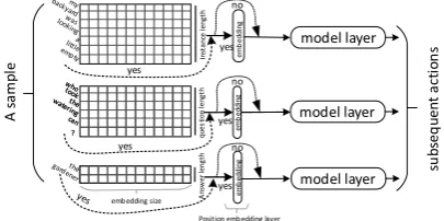
Figure 2: The input structure of the submodel
2https://github.com/xgli/word2vec-api
2.1 Similar input structures
Figure 2 shows the architecture of the sub models input. The input part of all sub models uses this structure. Within the structure, two flag variables are used to control the use of word embedding. One is whether to use the position embedding, and the other is to control whether or not the trained word embedding is used. From this structure, data flow to the subsequent network layer such as the classic model layer CNN, LSTM, BiLSTM and Attention.
2.2 The merge layer
In order to combine three text feature information, we have a merge layer in all of our sub models. The merge layer of these sub models is almost the same. Only the attention layer merge is dif-ferent from other sub models. The merge of most sub models first combines the instance matrix data with the question in sum operation, while combin-ing the matrix data with the answer, and finally combining the two sets of matrix data in thedot
operation. However, in the sub model with Atten-tion, merge layer combines the matrix data of the three texts withdotoperation. Next, we will focus on two sub models using classical models,while the rest of the other part of each sub models are similar to the two models.
2.3 Based on multi-BiLSTM+CNN model
Long short-term memory (LSTM or BiLSTM) is applied to text classification ((Liu et al.,2016) and (Lai et al.,2015)). The Convolutional Neural Net-works (CNN) is for local feature extraction ( Le-Cun et al.,1998). CNN can achieve good results in the semantic analysis (Yih et al.,2014), and other traditional NLP tasks (Collobert et al., 2011), es-pecially in sentiment analysis and question clas-sification (Kim et al., 2016). It is our novelty to combine CNN with multiple layers of BiLSTM with BiLSTM in front.
them into CNN1D layer. Finally, we use the Soft-max classifier to predict the results. Other sub models that do not use Attention are similar to the sub model structure, instead of replacing CNN1D with other structures.
2.4 Based on Attention + BiLSTM model
Attention is mostly used for document categoriza-tion (Yang et al., 2016).The model architecture is different from the multi-BiLSTM+CNN archi-tecture of word embedding layer. The structure of this model is roughly: a word embedding in-put structure, followed by attention layer which include the merge layer. Next to the batch nor-malization layer, BiLSTM layer , Softmax layer. We do a position embedding operation before in-putting the word embedding into attention layer. According to (Vaswani et al., 2017), the formula for constructing Position Embedding is as follows:
(
P E2i(p)=sin(p/100002i/dpos)
P E2i+1(p)=sin(p/100002i/dpos) (1)
Here is to map the positionpto the position vec-tor ofdpos dimension. The value of theith ele-ment of this vector isP Ei(p). Word embedding
first goes through the position embedding layer which is included in the architecture of the sub model input. Then the feature data enters into at-tention layer. In atat-tention layer, weights and bias are randomly added to position embedding and ex-cess numbers are masked as zero. We do batch normalization for the data coming out of attention layer, then input them into BiLSTM. Similarly, the results are obtained after Softmax layer.
3 Data Preparation
Although official data is regular, we have done a further normalization. All data set used by each model undergoes the following preprocess-ing steps:
1) The texts were lowercased
2) Using NLTK to tokenize each text
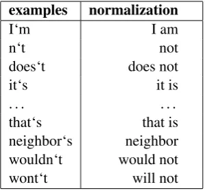
3) Abbreviations:
We’re very careful about the abbreviation, as ”’s” in ”it’s time for me to take her out.” is not the same as ”s” in ”Tom’s dad ordered pizza yesterday for the family.” We treat the first ”s”
examples normalization
I‘m I am
n‘t not
does‘t does not
it‘s it is
. . . .
[image:3.595.342.492.62.201.2]that‘s that is neighbor‘s neighbor wouldn‘t would not wont‘t will not
Table 1: normalization patterns.
as ”is,” and the second, of course, is an adjec-tive. We restore those abbreviations in Table 1 to normal forms.
4) Removing other characters:
Removing other characters, such as “!”,“% ”,“?”, “#”, “”,“@” Etc. Of course, not all other symbols that seem useless are removed. Like “$” are not removed.
4 Experiments and Results
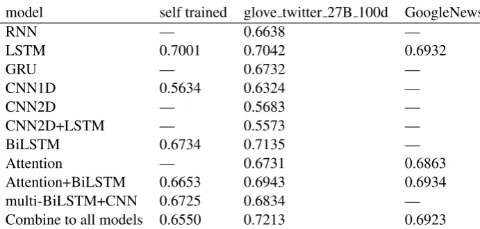
In order to optimize our network, we use (Kingma and Ba, 2014) optimizer on training model. All our experiments have been developed using an open source software library of Tensorflow with CUDA enabled, and run on a computer with In-tel Core(TM) i3 CPU 760 @2.8GHz, 8GB of RAM and GeForce GTX960 GPU. Due to the lack of hardware capacity, we do not run the en-tire system in one time. Instead, we run sin-gle model each time with different word embed-dings. When we use the word embedding of Google News 300d on some sub models, the sys-tem gives memory exhausted, and we switch to a smaller glove 27B 100d to run successfully. Ta-ble 2 shows our results for various models. As it can be seen from the table, ensemble results from the more different models get better results when other conditions are similar. Here we ensem-ble these models: RNN, GRU, BiLSTM, multi-BiLSTM+CNN and Attention+BiLSTM, based on their high accuracy. The dropout probability is 0.6 in each model, and the initial learning rate is 0.01.
5 Conclusion
model self trained glove twitter 27B 100d GoogleNews 300d.bin
RNN — 0.6638 —
LSTM 0.7001 0.7042 0.6932
GRU — 0.6732 —
CNN1D 0.5634 0.6324 —
CNN2D — 0.5683 —
CNN2D+LSTM — 0.5573 —
BiLSTM 0.6734 0.7135 —
Attention — 0.6731 0.6863
[image:4.595.100.446.60.225.2]Attention+BiLSTM 0.6653 0.6943 0.6934 multi-BiLSTM+CNN 0.6725 0.6834 — Combine to all models 0.6550 0.7213 0.6923
Table 2: Result for various models on task data set.
performance of a single model is poorer than the ensemble model. And the bigger the difference between the models, the higher performance the ensemble model makes. Still our results are less satisfying than top teams on the leaderboard. We will adjust the model, improve the hardware con-figuration of the computer, collect more external data, and do more experiments to get a better re-sult in the future.
Acknowledgments
This work was supported by the Natural Science Foundation of China No.61463050, No.61702443, No.61762091, the NSF of Yunnan Province No.2015FB113, the Project of Innovative Re-search Team of Yunnan Province.
References
Eric Breck, Yejin Choi, and Claire Cardie. 2007.
Iden-tifying expressions of opinion in context. In
Inter-national Joint Conference on Artificial Intelligence, pages 2683–2688.
Billy Chiu, Gamal Crichton, Anna Korhonen, and Sampo Pyysalo. 2016. How to train good word
embeddings for biomedical nlp. In Proceedings of
the 15th Workshop on Biomedical Natural Language Processing, pages 166–174.
Ronan Collobert, Jason Weston, L´eon Bottou, Michael Karlen, Koray Kavukcuoglu, and Pavel Kuksa. 2011. Natural language processing (almost) from
scratch. Journal of Machine Learning Research,
12(Aug):2493–2537.
Yoon Kim. 2014. Convolutional neural networks for
sentence classification. InProceedings of the 2014
Conference on Empirical Methods in Natural Lan-guage Processing (EMNLP), pages 1746–1751.
Yoon Kim, Yacine Jernite, David Sontag, and Alexan-der M Rush. 2016. Character-aware neural language
models. InAAAI, pages 2741–2749.
Diederik P Kingma and Jimmy Ba. 2014. Adam: A
method for stochastic optimization. In International
Conference on Learning Representations (ICLR).
Siwei Lai, Liheng Xu, Kang Liu, and Jun Zhao. 2015. Recurrent convolutional neural networks for text
classification. In AAAI, volume 333, pages 2267–
2273.
Yann LeCun, L´eon Bottou, Yoshua Bengio, and Patrick Haffner. 1998. Gradient-based learning applied to
document recognition. Proceedings of the IEEE,
86(11):2278–2324.
Pengfei Liu, Xipeng Qiu, and Xuanjing Huang. 2016. Recurrent neural network for text classification with
multi-task learning. InInternational Joint
Confer-ence on Artificial IntelligConfer-ence, pages 2873–2879.
Tomas Mikolov, Ilya Sutskever, Kai Chen, Greg S Cor-rado, and Jeff Dean. 2013. Distributed representa-tions of words and phrases and their
compositional-ity. InAdvances in neural information processing
systems, pages 3111–3119.
Frederic Morin and Yoshua Bengio. 2005. Hierarchi-cal probabilistic neural network language model. In
Aistats, volume 5, pages 246–252.
Michaela Regneri, Alexander Koller, and Manfred Pinkal. 2010. Learning script knowledge with web
experiments. InMeeting of the Association for
Com-putational Linguistics, pages 979–988.
Warren S. Sarle. 1995. Stopped training and other
remedies for overfitting. In Proceedings of
Sympo-sium on the Interface, pages 352–360.
Richard Socher, Jeffrey Pennington, Eric H Huang, Andrew Y Ng, and Christopher D Manning. 2011. Semi-supervised recursive autoencoders for
predict-ing sentiment distributions. InConference on
Em-pirical Methods in Natural Language Processing, EMNLP 2011, 27-31 July 2011, John Mcintyre Con-ference Centre, Edinburgh, Uk, A Meeting of Sigdat, A Special Interest Group of the ACL, pages 151–161.
Nitish Srivastava, Geoffrey Hinton, Alex Krizhevsky, Ilya Sutskever, and Ruslan Salakhutdinov. 2014. Dropout: a simple way to prevent neural networks
from overfitting. Journal of Machine Learning
Re-search, 15(1):1929–1958.
Ashish Vaswani, Noam Shazeer, Niki Parmar, Jakob Uszkoreit, Llion Jones, Aidan N Gomez, Ł ukasz Kaiser, and Illia Polosukhin. 2017. Attention is all
you need. In I., editor,Advances in Neural
Informa-tion Processing Systems 30, pages 5998–6008.
Zichao Yang, Diyi Yang, Chris Dyer, Xiaodong He, Alex Smola, and Eduard Hovy. 2016. Hierarchi-cal attention networks for document classification. InProceedings of the 2016 Conference of the North American Chapter of the Association for Computa-tional Linguistics: Human Language Technologies, pages 1480–1489.
Ainur Yessenalina and Claire Cardie. 2011. Compo-sitional matrix-space models for sentiment
analy-sis. In Conference on Empirical Methods in
Natu-ral Language Processing, EMNLP 2011, 27-31 July 2011, John Mcintyre Conference Centre, Edinburgh, Uk, A Meeting of Sigdat, A Special Interest Group of the ACL, pages 172–182.
Wen-tau Yih, Xiaodong He, and Christopher Meek. 2014. Semantic parsing for single-relation
ques-tion answering. InProceedings of the 52nd Annual
Meeting of the Association for Computational Lin-guistics (Volume 2: Short Papers), volume 2, pages 643–648.
Wen-tau Yih, Kristina Toutanova, John C Platt, and Christopher Meek. 2011. Learning discriminative
projections for text similarity measures. In