Proceedings of NAACL-HLT 2018, pages 767–776
Automatic Stance Detection Using End-to-End Memory Networks
Mitra Mohtarami1, Ramy Baly1, James Glass1, Preslav Nakov2
Lluís Màrquez3∗, Alessandro Moschitti3∗
1MIT Computer Science and Artificial Intelligence Laboratory, Cambridge, MA, USA 2Qatar Computing Research Institute, HBKU, Doha, Qatar;3Amazon
{mitra,baly,glass}@csail.mit.edu
[email protected]; {lluismv,amosch}@amazon.com
Abstract
We present an effective end-to-end memory network model that jointly (i) predicts whether a given document can be considered as rele-vant evidence for a given claim, and (ii) ex-tracts snippets of evidence that can be used to reason about the factuality of the target claim. Our model combines the advantages of con-volutional and recurrent neural networks as part of a memory network. We further in-troduce a similarity matrix at the inference level of the memory network in order to ex-tract snippets of evidence for input claims more accurately. Our experiments on a pub-lic benchmark dataset, FakeNewsChallenge, demonstrate the effectiveness of our approach.
1 Introduction
Recently, an unprecedented amount of false infor-mation has been flooding the Internet with aims ranging from affecting individual people’s beliefs and decisions (Mihaylov et al., 2015; Mihaylov and Nakov,2016) to influencing major events such as political elections (Vosoughi et al.,2018). Con-sequently, manual fact checking has emerged with the promise to support accurate and unbiased anal-ysis of rumors spreading in social medias, as well as of claims made by public figures or news media. As manual fact checking is a very tedious task, automatic fact checking has been proposed as a possible alternative. This is often broken into in-termediate steps in order to alleviate the task com-plexity. One such step isstance detection, which is also useful for human experts as a stand-alone task. The task aims to identify the relative per-spective of a piece of text with respect to a claim, typically modeled using labels such asagree, dis-agree,discuss, andunrelated; Figure1gives some examples.
∗Work conducted while these authors were at QCRI.
Claim: Robert Plant Ripped up $800M Led Zeppelin Re-union Contract.
Stance Snippet
agree Led Zeppelin’s Robert Plant turned down £500m to reform supergroup...
disagree Robert Plant’s publicist has described as “rub-bish” a Daily Mirror report that he rejected a £500m Led Zeppelin reunion...
discuss Robert Plant reportedly tore up an $800 million Led Zeppelin reunion deal...
unrelated Richard Branson’s Virgin Galactic is set to launch SpaceShipTwo today...
Figure 1: Examples of snippets of text and their stance with respect to the target claim.
Here, we address the problem of stance detection using a novel model based on end-to-end memory networks (Sukhbaatar et al.,2015), which incorpo-rates convolutional and recurrent neural networks, as well as a similarity matrix. Our model jointly addresses the problems of predicting the stance of a text with respect to a given claim, and of extract-ing relevant text snippets as support for the predic-tion of the model. We further introduce a similar-ity matrix, which we use at inference time in order to improve the extraction of relevant snippets.
The experimental results on the Fake News Challenge benchmark dataset show that our model, which is very feature-light, performs close to the state of the art. Our contributions can be summarized as follows: (i) We apply a novel memory network model enhanced with CNN and LSTM networks for stance detection. (ii) We fur-ther propose a novel extension of the general ar-chitecture based on a similarity matrix, which we use at inference time, and we show that this exten-sion offers sizable performance gains. (iii) Finally, we show that our model is capable of extracting meaningful snippets from a given text document, which is useful not only for stance detection, but more importantly can support human experts who need to decide on the factuality of a given claim.
2 Stance Detection Memory Networks Long-term memory is necessary to determine the stance of a long document with respect to a claim, as relevant parts of a document—paragraphs or text snippets—can indicate the perspective of a document with respect to a claim. Memory net-works have been designed to remember past in-formation (Sukhbaatar et al., 2015) and they can be particularly well-suited for stance detection since they can use a variety of inference strategies alongside their memory component.
In this section, we present a novel memory net-work for stance detection. It contains a new infer-ence component that incorporates a similarity ma-trix to extract, with better accuracy, textual snip-pets that are relevant to the input claims.
2.1 Overview of the network
A memory network is a 5-tuple{M, I, G, O, R},
where thememoryM is a sequence of objects or
representations, the input I is a component that
maps the input to its representation, the general-izationcomponentG(Sukhbaatar et al.,2015)
up-dates the memory with respect to new input, the output O generates an output for each new input
and the current memory state, and finally, the re-sponse R converts the output into a desired
re-sponse format, e.g., a textual rere-sponse or an ac-tion. These components can potentially use many different machine learning models.
Our new memory network for stance detection is a 6-tuple {M, I, F, G, O, R}, where F
repre-sents the new inference component. It takes an input documentdas evidence and a textual
state-mentsas a claim and converts them into their
cor-responding representations in the inputI. Then, it
passes them to the memoryM. Next, the relevant
parts of the input are identified in F, and
after-wards they are used by Gto update the memory.
Finally, O generates an output from the updated
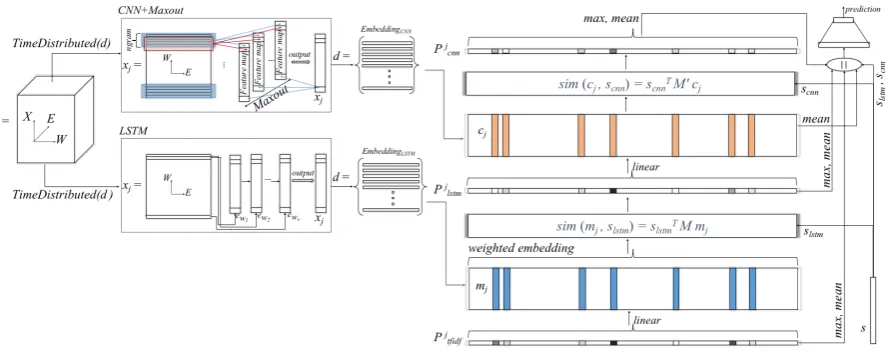
memory, and converts it to a desired response for-mat withR. The network architecture is depicted
in Figure2. We describe the components below.
2.2 Input Representation Component
The input to the stance detection algorithm is a document d as evidence and a textual statement sas a claim, (see lines 2 and 3 in Table1). Eachd
is segmented into paragraphsxj of varied lengths,
where eachxjis considered as a piece of evidence
for stance detection.
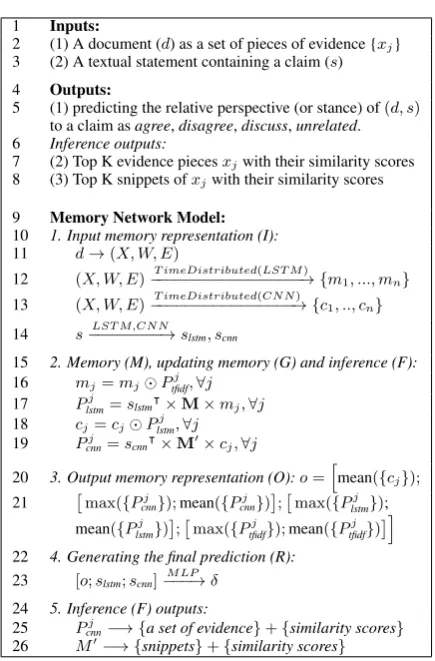
1 Inputs:
2 (1) A document (d) as a set of pieces of evidence {xj} 3 (2) A textual statement containing a claim (s) 4 Outputs:
5 (1) predicting the relative perspective (or stance) of(d, s) to a claim asagree,disagree,discuss,unrelated. 6 Inference outputs:
7 (2) Top K evidence piecesxjwith their similarity scores 8 (3) Top K snippets ofxjwith their similarity scores
9 Memory Network Model:
10 1. Input memory representation (I):
11 d→(X, W, E)
12 (X, W, E)−−−−−−−−−−−−−−−−−→ {T imeDistributed(LST M) m1, ..., mn} 13 (X, W, E)−−−−−−−−−−−−−−−−→ {T imeDistributed(CN N) c1, .., cn} 14 s−−−−−−−−→LST M,CN N slstm, scnn
15 2. Memory (M), updating memory (G) and inference (F): 16 mj=mjPtfidfj ,∀j
17 Plstmj =slstm|×M×mj,∀j 18 cj=cjPlstmj ,∀j 19 Pj
cnn=scnn|×M0×cj,∀j
20 3. Output memory representation (O):o=hmean({cj}); 21 max({Pj
cnn});mean({Pcnnj });max({Plstmj }); mean({Plstmj });max({Ptfidfj });mean({Ptfidfj })i 22 4. Generating the final prediction (R):
23 [o;slstm;scnn]−−−→M LP δ 24 5. Inference (F) outputs: 25 Pj
[image:2.595.309.527.54.385.2]cnn−→ {a set of evidence}+{similarity scores} 26 M0−→ {snippets}+{similarity scores}
Table 1: Summary of our memory network algorithm for stance detection.
Indeed, a paragraph usually presents a coherent ar-gument, unified under one or more inter-related topics. The input component in our model con-verts eachdinto a set of pieces of evidence in a
three dimensional (3D) tensor space as shown be-low (see line 11 in Table1):
d= (X, W, E) (1)
where X = {x1, ..., xn} is a set of paragraphs
considered as pieces of evidence; each xj is
rep-resented by a set of wordsW = {w1, ..., wv}—
drawn from a global vocabulary of sizev—and a set of neural representationsE = {e1, ..., ev}for
words inW. This 3D space is illustrated as a cube
in Figure2.
Eachxjis encoded from the 3D space into a
se-mantic representation at the input component us-ing a Long Short-Term Memory (LSTM) network. The lower left component in Figure 2shows our LSTM network, which operates on our input as follows (see also line 12 in Table1):
(X, W, E)−−−−−−−−−−−−−−−−→ {T imeDistributed(LST M) m1, ..., mn}
Figure 2: The architecture of our memory network model for stance detection.
wheremj is the LSTM representation ofxj, and
TimeDistributed()indicates a wrapper that enables training the LSTM over all pieces of evidence by applying the same LSTM model to each time-step of a 3D input tensor, i.e.,(X, W, E).
While LSTM networks were designed to ef-fectively capture and memorize their inputs (Tan et al., 2016), Convolutional Neural Networks (CNNs) emphasize the local interaction between the individual words in the input word sequence, which is important for obtaining an effective rep-resentation. Here, we use a CNN in order to en-code each xj into its representation cj as shown
below (see line 13 in Table1).
(X, W, E)−−−−−−−−−−−−−−−→ {T imeDistributed(CN N) c1, .., cn}
(3) As shown in the left-top corner of Figure2, this representation is passed as a new input to the com-ponentM of our memory network model.
More-over, we keep track of the computedn-grams from the CNN so that we can use them later in the in-ference and in the response components (see sec-tions 2.3 and 2.6). For this purpose, we use a Maxout layer (Goodfellow et al.,2013) to take the maximum acrosskaffine feature maps computed
by the CNN, i.e., pooling across channels.
Previous work investigated the combination of convolutional and recurrent representations, which were fed to the other network as input (Tan et al.,2016;Donahue et al.,2015;Zuo et al.,2015;
Sainath et al.,2015). In contrast, we feed individ-ual outputs into our memory network separately, and we let it decide which representation better helps the target task. We demonstrate the effec-tiveness of this choice in our experiments.
Furthermore, we convert each input claims into
its representation using the corresponding LSTM and CNN networks as follows:
s−−−−−−−−→LST M,CN N slstm, scnn (4) where slstm andscnn are the representations of s computed usingLST M andCN N networks,
re-spectively. Note that these are separate networks with different parameters from those used to en-code the pieces of evidence.
Lines 10–14 of Table1describe the above steps in representing I in our memory network. This
component encodes each input document d into
a set of pieces of evidence {xj}∀j: it computes
LSTM and CNN representations, mj andcj,
re-spectively, for eachxj, and LSTM and CNN
rep-resentations,slstmandscnn, for each claims. 2.3 Inference Component
The resulting representations can serve to compute semantic similarity between claims and pieces of evidence. We define the similarityPlstmj betweens
andxj as follows (see line 17 in Table1):
Plstmj =slstm|×M×mj,∀j (5)
whereslstm ∈Rqandmj ∈Rdare the LSTM
rep-resentations of sand xj, respectively, and M ∈ Rq×dis a similarity matrix capturing their
similar-ity. For this purpose, M mapss andxj into the
same space as shown in Figure3. M is a set of q×dparameters of the network, which are
opti-mized during the training.
In a similar fashion, we compute the similarity
Pcnnj betweenxj andsusing the CNN
representa-tions as follows (see line 19 in Table1):
s
: (
slstm , scn
n
)
M
s' xj: (mj, cj)
sim(slstm, mj)
or
[image:4.595.75.289.64.135.2]sim(scnn, cj)
Figure 3: Matching a claimsand a piece of evidence xjusing a similarity matrixM. Here,slstmandscnnare
the LSTM and CNN representations ofs, whereasmj
andcjare the LSTM and CNN representations ofxj.
wherescnn ∈ Rq0 andcj ∈ Rd0 are the
represen-tations of s and xj obtained with CNN,
respec-tively. The similarity matrix M0 ∈ Rq0×d0 is a set of q0 ×d0 parameters of the network and is
optimized during the training. Plstmj andPcnnj in-dicate the claim-evidence similarity vectors com-puted based on the LSTM and on the CNN repre-sentations ofsandxj, respectively.
The rationale behind using the similarity matrix is that in our memory network model, as Figure3
shows, we seek a transformation of the input claim such thats0 =M×sin order to obtain the closest
facts to the claim.
In fact, the relevant parts of the input document with respect to the input claim can be captured at a different level, e.g., using M0 for the n-gram
level or using the claim-evidencePlstmj orPcnnj ,∀j at the paragraph level. We note that (i)Plstmj uses
LSTM to take the word order and long-length de-pendencies into account, and (ii) Pcnnj uses CNN to take n-grams and local dependencies into
ac-count, as explained in sections 2.2 and2.3. Ad-ditionally, we compute another semantic similar-ity vector, Ptfidfj , by applying a cosine similarity
between the TF.IDF (Spärck Jones, 2004) repre-sentation of xj ands. This is particularly useful
for stance detection as it can help detect unrelated pieces of evidence.
2.4 Memory and Generalization Components The information flow and updates in the mem-ory is as follows: first, the representation vector
{mj}∀j is passed to the memory and updated
us-ing the claim-evidence similarity vector{Ptfidfj }:
mj =mjPtfidfj ,∀j (7)
The reason for this weighting is to filter out most unrelated evidence with respect to the claim. The updated mj in conjunction with slstm are used by the inference component–componentF to
compute{Plstmj }as explained in Section2.3.
Then,{Plstmj } is used to update the new input set
{cj}∀jto the memory:
cj =cjPlstmj ,∀j (8)
Finally, the updatedcj in conjunction withscnn are used to computePcnnj as explained in Sec.2.3. 2.5 Output Representation Component In memory networks, the memory output depends on the final goal, which, in our case, is to detect the relative perspective of a document to a claim. For this purpose, we apply the following equation:
o=hmean({cj});
max({Pcnnj });mean({Pcnnj });max({Plstmj });
mean({Plstmj });max({Ptfidfj });mean({Ptfidfj })i (9) where mean({cj})is the average vector ofcj
rep-resentations. Furthermore, we compute the max-imum and the average similarity between each piece of evidence and the claim usingPtfidfj ,Plstmj
andPcnnj , which are computed for each evidence and claim in the inference component F. The
maximum similarity identifies the part of docu-mentxjthat is most similar to the claim, while the
average similarity measures the overall similarity between the document and the claim.
2.6 Response and Output Generation
This component computes the final stance of a document with respect to a claim. For this pur-pose, the concatenation of vectorso,slstmandscnn is fed into a Multi-Layer Perceptron (MLP), where a softmax predicts the stance of the document with respect to the claim, as shown below (see also lines 22–23 in Table1):
[o;slstm;scnn]−−−→M LP δ (10)
whereδ is a softmax function. In addition to the
resulting stance, we extract snippets from the in-put document that best indicate the perspective of the document with respect to the claim. For this purpose, we usePcnnj andM0as explained in Sec-tion2.3(see also lines 24–26 in Table1).
The overall model is shown in Figure 2 and a summary of the model is presented in Table1. All the model parameters, including those of (i) CNN and LSTM in I, (ii) the similarity matrices M
andM0 inF, and (iii) the MLP inR, are jointly
3 Experiments and Evaluation 3.1 Data
We use the dataset provided by the Fake News Challenge,1 where each example consists of a claim–document pair with the following possi-ble relations between them: agree(the document agrees with the claim), disagree (the document disagrees with the claim), discuss (the document discusses the same topic as the claim, but does not take a stance with respect to the claim),unrelated (the document discusses a different topic than the topic of the claim). The data includes a total of 75.4K claim–document pairs, which link 2.5K unique articles with 2.5K unique claims, i.e., each claim is associated with 29.8 articles on average. 3.2 Settings
We use 100-dimensional word embeddings from GloVe (Pennington et al., 2014), which were trained on two billion tweets. We further use Adam as an optimizer and categorical cross-entropy as a loss. We use 100-dimensional units for the LSTM embeddings, and 100 feature maps with filter width of 5 for the CNN. We consider the firstp= 9 paragraphs for each document, wherep
is the median of the number of paragraphs. We optimize the hyper-parameters of the mod-els using a validation dataset (20% of the training data). Finally, as the data is largely imbalanced to-wards theunrelatedclass, during training, we ran-domly select an equal number of instances from each class at each epoch.
3.3 Evaluation Measures
We use the following evaluation measures: Accuracy: The number of correctly classified examples divided by the total number of examples. It is equivalent to micro-averaged F1.
Macro-F1: We calculate F1for each class, and
then we average across all classes.
Weighted Accuracy: This is a weighted, two-level scoring scheme, which is applied to each test example. First, if the example is from the un-related class and the model correctly predicts it, the score is incremented by 0.25; otherwise, if the example isrelated and the model predictsagree, disagree, ordiscuss, the score is incremented by 0.25. Second, there is a further increment by 0.75 for eachrelatedexample if the model predicts the correct label:agree,disagree, ordiscuss.
1Available atwww.fakenewschallenge.org
Finally, the score is normalized by dividing it by the total number of test examples. The ra-tionale behind this metric is that the binary re-lated/unrelatedclassification task is expected to be much easier, while also being arguably less rele-vant to fake news detection than the stance detec-tion task, which aims to further classify relevant instances as agree, disagree, or discuss. There-fore, the former task is given less weight and the latter task is given more weight through the weighted accuracy metric.
3.4 Baselines
Given the imbalanced nature of our data, we use two baselines in which we label all testing exam-ples with the same label: (i)unrelatedand (ii) dis-cuss. The former is the majority class baseline, which is a reasonable baseline for Accuracy and macro-F1, while the latter is a potentially better
baseline forWeighted Accuracy.
We further use CNN and LSTM, and combina-tions thereof as baselines, since they form compo-nents of our model, and also because they yield state-of-the-art results for text, image, and video classification (Tan et al., 2016; Donahue et al.,
2015;Zuo et al.,2015;Sainath et al.,2015). Finally, we include the official baseline from the challenge, which is a Gradient Boosting classifier with word andn-gram overlap features, as well as
indicators for refutation and polarity.
3.5 Our Models
sMemNN: This is our model presented in
Fig-ure 2. Note that unlike the CNN+LSTM and
the LSTM+CNN baselines above, which feed the output of one network into the other one, the sMemNN model feeds the individual outputs of both the CNN and the LSTM networks into the memory network, and lets it decide how much to rely on each of them. This consideration also facil-itates reasoning and explaining model predictions, as we will discuss in more detail below.
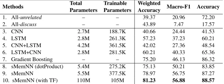
Methods TotalParameters TrainableParameters WeightedAccuracy Macro-F1 Accuracy
1. All-unrelated – – 39.37 20.96 72.20
2. All-discuss – – 43.89 7.47 17.57
3. CNN 2.7M 188.7K 40.66 24.44 41.53
4. LSTM 2.8M 261.3K 57.23 37.23 60.21
5. CNN+LSTM 4.2M 361.5K 42.02 27.36 48.54
6. LSTM+CNN 2.8M 281.5K 60.21 40.33 65.36
7. Gradient Boosting – – 75.20 46.13 86.32
8. sMemNN (dotProduct) 5.4M 275.2K 75.13 50.21 83.85
9. sMemNN 5.5M 377.5K 78.97 56.75 87.27
[image:6.595.117.486.63.202.2]10. sMemNN (with TF) 110M 105M 81.23 56.88 88.57
Table 2: Evaluation results on the test data.
sMemNN (with TF): Since our LSTM and CNN networks use a limited number of starting paragraphs2for an input document, we enrich our model with the BOW representation of documents and claims as well as their TF.IDF-based cosine similarity. We concatenate these vectors with the memory outputs (section 2.5) and pass them to the R component (section 2.6) of sMemNN. We expect these BOW vectors provide useful infor-mation that are not initially incorporated into the sMemNN model.
3.6 Results
Table2 reports the performance of all models on the test dataset. The All-unrelated and the All-discuss baselines perform poorly across the eval-uation measures, except for All-unrelated, which achieves high accuracy, which is due tounrelated being by far the dominant class in the dataset.
Next, we can see that the LSTM model consis-tently outperforms the CNN across all evaluation measures. Although the larger number of parame-ters of the LSTM can play a role, we believe that its superiority comes from it being able to remem-ber previously observed relevant pieces of text.
Next, we see systematic improvements for the combinations of the CNN and the LSTM mod-els: CNN+LSTM is better than CNN alone, and LSTM+CNN is better than LSTM alone. Bet-ter performance is achieved by the LSTM+CNN model, where claims and evidence are first pro-cessed by a LSTM and then fed into a CNN.
The Gradient Boosting model achieves sizable improvement over the above baseline neural mod-els. However, we should note that these neural models do not have the rich hand-crafted features that were used in the Gradient Boosting model.
2Due to the long length of documents, it is impractical to
consider all paragraphs when training LSTM and CNN.
Row 9 shows the results for our memory net-work model (sMemNN), which consistently out-performs all other baseline models across all eval-uation metrics, achieving 10.62 and 3.77 points of absolute improvement in terms of Macro-F1 and Weighted Accuracy, respectively, over the best baseline (Gradient Boosting). We believe this is due to the memory network being able to capture good text snippets. As we will see below, these snippets are also useful for explaining the model’s predictions. Comparing row 9 to row 8, we can see the importance of our proposed similarity ma-trix: replacing that matrix by a simple dot product hurts the performance of the model considerably across all evaluation measures, thus lowering it to the level of the Gradient Boosting model.
Finally, row 10 shows the results for our mem-ory network model enriched by BOW representa-tion. As we expected, it improves the performance of sMemNN - perhaps by capturing useful infor-mation from paragraphs beyond the starting few.
To put the results of sMemNN in perspective, we should mention that the best system at the Fake News Challenge (Baird et al., 2017) achieved a macro-F1 of 57.79, which is not significantly dif-ferent from our results at the 0.05 significance level (p-value=0.53). Yet, they have an ensemble combining the feature-rich Gradient Boosting sys-tem with neural networks. In contrast, we only use raw text as input and no ensembles, and our main goal is to study a new memory network model and its explainability component.
Claim 1:man saved from bear attack - thanks to his justin bieber ringtone Evidence Id Pj
cnn Evidence Snippet
2069-3 0.89 ... fishing in the yakutia republic , russia , igor vorozhbitsyn is lucky to be alive after his justin bieber ringtone , baby , scared off a bear that was attacking him0.41... 2069-7 1.0 ... but as the bear clawed vorozhbitsyn ’ s face and back his mobile phone rang
, the ringtone selected was justin bieber ’ s hit song baby . rightly startled1.00 , the bear retreated back into0.39the forest ...
true label:agree;predicted label:agree
Claim 2:50ft crustacean , dubbed crabzilla , photographed lurking beneath the waters in whitstable Evidence Id Pj
cnn Evidence Snippet
24835-1 0.0046 ... a marine biologist has killed off claims-0.0008 that a giant crab is0.0033living on the kent coast - insisting the image is probably a well - doctored hoax0.0012...
24835-7 -0.0008 ... i don ’ t know what the currents are like around that harbour or what sort of they might produce in the sand , but i think it ’ s more conceivable that someone is playing0.0007 about with the photo ...
[image:7.595.83.511.64.262.2]true label:disagree;predicted label:disagree
Table 3: Examples of highly ranked snippets of evidence for an input claim, which are automatically extracted by our inference component. ThePj
cnncolumn and the values in the top-right corner of the highlighted snippets show
the similarity between the claim and evidence, and between the claim and snippets of the evidence, respectively.
0 10 20 30 40 50 60 70 80 epochs
0.0 0.2 0.4 0.6 0.8 1.0 1.2 1.4
coverage
unrelated discuss agree disagree
0.2 0.4 0.6 0.8 1.0 1.2 1.4
loss
val_loss
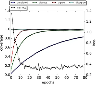
Figure 4: Effect of data coverage. The lefty-axis shows the fraction of data observed during training (cover-age), the righty-axis shows the loss during training.
This is mainly because the document that dis-cusses a claim often shares the same topic with the claim, but then it does not take a stance with respect to that claim. (iii) Thedisagreeexamples are the most difficult ones for all models, probably because they represent by far the smallest class.
4 Discussion
4.1 Training Data Coverage
As discussed previously, we balance the data at each training iteration by randomly selectingz
in-stances from each of the four target classes, where
zis the size of the class with the minimum
num-ber of training instances. Here, we investigate the amount of training data that gets actually used.
For this purpose, at each training iteration, we re-port the prore-portion of the training instances from each class that have been used for training so far, either at the current or at any of the previous iter-ations. As Figure4shows, our random data sam-pling procedure eventually covers almost all train-ing instances. Since thedisagreeclass is the small-est, its instances remain fully covered through-out the process. Moreover, almost all other re-lated instances, i.e., agree and discuss, are ob-served during training, as well as a large fraction of the dominatingunrelated examples. Note that the model achieves its best (lowest) loss on the val-idation dataset at iteration 31, when almost all re-lated training instances are observed. This hap-pens while the corresponding fraction for the un-related pairs is around 50%, i.e., a considerable number of theunrelatedinstances are not required to be used for training.
4.2 Explainability
One of the main advantages of our memory net-work model, compared to the baselines and to re-lated work in general, is that it has the capacity to explain its predictions by extracting snippets from each piece of evidence that supports its pre-diction. As we explained in Section 2.3, our in-ference component predicts the similarity between each piece of evidencexjand the claimsat then
-grams level using the similarity matrixM0and the
claim-evidence similarity vectorPcnnj . Below, we
[image:7.595.86.274.327.494.2]1 2 3 4 5 rank
0.15 0.20 0.25 0.30 0.35 0.40
precision
agree disagree overall
(a) n-grams
1 2 3 4 5 rank
0.15 0.20 0.25 0.30 0.35 0.40 0.45 0.50
precision
agree disagree overall
(b) consecutiven-grams
1 2 3 4 5 rank
0.35 0.40 0.45 0.50 0.55 0.60 0.65 0.70
precision
agree disagree overall
[image:8.595.75.520.68.216.2](c) sentences
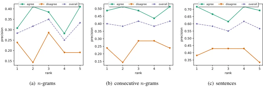
Figure 5: Prediction explainability. Sub-figures (a)-(c) show the precision of our model at explaining its predictions when the pieces of evidence are (a) fixed-lengthn-grams (n= 5), (b) combinations of several consecutiven-grams with similar scores, or (c) the entire sentence, if it includes at least one extractedn-gram snippet.
Table 3 shows examples of two claims and the snippets extracted as evidence. Column Pcnnj
shows the overall similarity between the evidence and the corresponding claim as computed by the inference component of our model. The high-lighted texts are the snippets with the highest sim-ilarity to the claim as extracted by the same com-ponent. The values on the snippets’ top-right show the claim-snippet similarity values obtained by the inference component.
Note that all snippets are fixed-length, namely 5-grams; however, in case there are several con-secutiven-grams with similar scores, for better
il-lustration, we combine them into a single snippet and we report their average values (see the snippet for evidence 2069-3). As these examples show, our model can accurately predict the stance of these pieces of evidence against their correspond-ing claims. Also, claim 2 and its correspondcorrespond-ing evidence are shown at the second row of Table3. As this example shows, the similarity values asso-ciated with snippets are either too small or nega-tive, e.g., see the similarity value for the snippet “biologist has killed off claims.” We can see that these help the model to make accurate predictions. We conduct the following experiment to quan-tify the performance of our memory network at explaining its predictions: we randomly sam-ple 100agree/disagreeclaim–document examples from our gold data, and we manually evaluate the top five pieces of evidence that our model provides to support/oppose the corresponding claims.3
3In 76 cases, our model correctly classified the
agree/disagreeexamples when the evaluation was conducted, and it further provided arguably adequate snippets.
Figure 5(a) shows the precision of our memory network model at explaining its predictions when each supporting/opposing piece of evidence is an
n-gram snippet of fixed length (n = 5) for the agreeand thedisagreeclasses, and their combina-tions at the top-kranks,k ={1, . . . ,5}. We can see in the figure that the model achieves precision of 0.28, 0.32, 0.35, 0.25, and 0.33 at ranks 1–5. Moreover, we find that it can accurately identify useful key phrases such as officials declared the video,according to previous reports,believed will come,president in his tweetsas supporting pieces of evidence, andproved a hoax,shot down a cnn report, would be skeptical as opposing pieces of evidence.
Note that this relatively low precision of our memory network model at explaining its agree/disagreepredictions is mainly due to the un-supervised nature of this task as no gold snippets justifying the document’s gold stance with respect to the target claim are available in the Fake News Challenge dataset.4
Furthermore, our evaluation setup is at the n
-gram level in Figure5(a). However, if we conduct a more coarse-grained evaluation where we com-bine consecutiven-grams with similar scores into
a single snippet, the precision for these new snip-pets will improve to 0.40, 0.38, 0.42, 0.38, and 0.42 at ranks 1–5, as Figure5(b)shows. If we fur-ther extend the evaluation to the sentence level, the precision will jump to 0.60, 0.58, 0.55, 0.62, and 0.57 at ranks 1–5, as we can see in Figure5(c).
4Some other recent datasets, to be presented at this same
5 Related Work
While stance detection is an interesting task in its own right, e.g., for media monitoring, it is also an important component for fact checking and ve-racity inference.5 Automatic fact checking was envisioned by Vlachos and Riedel (2014) as a multi-step process that (i) identifies check-worthy statements (Hassan et al., 2015; Gencheva et al.,
2017;Jaradat et al.,2018), (ii) generates questions to be asked about these statements (Karadzhov et al.,2017), (iii) retrieves relevant information to create a knowledge base (Shiralkar et al., 2017), and (iv) infers the veracity of these statements, e.g., using text analysis (Castillo et al., 2011;
Rashkin et al.,2017) or information from external sources (Mihaylova et al.,2018;Karadzhov et al.,
2017;Popat et al.,2017).
There have been some nuances in the way re-searchers have defined the stance detection task. SemEval-2016 Task 6 (Mohammad et al., 2016) targets stances with respect to some target propo-sition, e.g., entities, concepts or events, as in-favor, against, or neither. The winning model in the task was based on transfer learning: a Re-current Neural Network trained on a large Twitter corpus was used to predict task-relevant hashtags and to initialize a second recurrent neural network trained on the provided dataset for stance predic-tion (Zarrella and Marsh, 2016). Subsequently,
Zubiaga et al.(2016) detected the stance of tweets toward rumors and hot topics using linear-chain conditional random fields (CRFs) and tree CRFs that analyze tweets based on their position in tree-like conversational threads.
Most commonly, stance detection is defined with respect to a claim, e.g., as in the 2017 Fake News Challenge. The best system in the chal-lenge was an ensemble of gradient-boosted de-cision trees with rich features (e.g., sentiment, word2vec, singular value decomposition (SVD) and TF.IDF features, etc.) and a deep convolu-tional neural network to address the stance detec-tion problem (Baird et al.,2017).
Unlike the above work, we use a feature-light memory network that jointly infers the stance and highlights relevant snippets of evidence with re-spect to a given claim.
5Yet, stance detection and fact checking are typically
sup-ported by separate datasets. Two notable upcoming excep-tions, both appearing in this HLT-NAACL’2018, are (Thorne et al.,2018) for English and (Baly et al.,2018) for Arabic.
6 Conclusion
We studied the problem of stance detection, which aims to predict whether a given document sup-ports, challenges, or just discusses a given claim. The nature of the task requires a machine learn-ing model to focus on the relevant paragraphs of the evidence. Moreover, in order to understand whether a paragraph supports a claim, there is a need to refer to information in other paragraphs. CNNs or LSTMs are not well-suited for this task as they cannot model complex dependencies such as semantic relationships with respect to entire previous paragraphs. In contrast, memory net-works are exactly designed to remember previous information. However, given the large size of doc-uments and paragraphs, basic memory networks do not handle well irrelevant and noisy informa-tion, which we confirmed in our experiments.
Thus, we proposed a novel extension of general memory networks based on a similarity matrix and a stance filtering component, which we apply at the inference level, and we have shown that this extension offers sizable performance gains mak-ing memory networks competitive. Moreover, our model can extract meaningful snippets from docu-ments that can explain the stance of a given claim. In future work, we plan to extend the inference component to select an optimal set of explanations for each prediction, and to explain the model as a whole, not only at the instance level.
Acknowledgment
This research was carried out in collaboration be-tween the MIT Computer Science and Artificial Intelligence Laboratory (CSAIL) and the HBKU Qatar Computing Research Institute (QCRI).
References
Sean Baird, Doug Sibley, and Yuxi Pan. 2017. Ta-los targets disinformation with fake news challenge victory. https://blog.talosintelligence.com/2017/06/ talos-fake-news-challenge.html.
Ramy Baly, Mitra Mohtarami, James Glass, Lluís Màrquez, Alessandro Moschitti, and Preslav Nakov. 2018. Integrating stance detection and fact checking in a unified corpus. InProceedings of HLT-NAACL. New Orleans, LA, USA.
Jeff Donahue, Lisa Anne Hendricks, Sergio Guadar-rama, Marcus Rohrbach, Subhashini Venugopalan, Trevor Darrell, and Kate Saenko. 2015. Long-term recurrent convolutional networks for visual recog-nition and description. In Proceedings of CVPR. Boston, MA, USA, pages 2625–2634.
Pepa Gencheva, Preslav Nakov, Lluís Màrquez, Al-berto Barrón-Cedeño, and Ivan Koychev. 2017. A context-aware approach for detecting worth-checking claims in political debates. InProceedings of RANLP. Varna, Bulgaria, pages 267–276. Ian J. Goodfellow, David Warde-Farley, Mehdi Mirza,
Aaron Courville, and Yoshua Bengio. 2013. Maxout networks. In Proceedings of ICML. Atlanta, GA, USA, pages 1319–1327.
Naeemul Hassan, Chengkai Li, and Mark Tremayne. 2015. Detecting check-worthy factual claims in presidential debates. In Proceedings CIKM. Mel-bourne, Australia, pages 1835–1838.
Israa Jaradat, Pepa Gencheva, Alberto Barrón-Cedeño, Lluís Màrquez, and Preslav Nakov. 2018. Claim-Rank: Detecting check-worthy claims in Arabic and English. In Proceedings of HLT-NAACL. New Or-leans, LA, USA.
Georgi Karadzhov, Preslav Nakov, Lluís Màrquez, Alberto Barrón-Cedeño, and Ivan Koychev. 2017. Fully automated fact checking using external sources. InProceedings of RANLP. Varna, Bulgaria, pages 344–353.
Todor Mihaylov, Georgi Georgiev, and Preslav Nakov. 2015. Finding opinion manipulation trolls in news community forums. InProceedings of CoNLL. Bei-jing, China, pages 310–314.
Todor Mihaylov and Preslav Nakov. 2016. Hunting for troll comments in news community forums. In Pro-ceedings of ACL. Berlin, Germany.
Tsvetomila Mihaylova, Preslav Nakov, Lluis Marquez, Alberto Barron-Cedeno, Mitra Mohtarami, Georgi Karadzhov, and James Glass. 2018. Fact checking in community forums. InProceedings of AAAI. New Orleans, LA, USA.
Saif Mohammad, Svetlana Kiritchenko, Parinaz Sob-hani, Xiao-Dan Zhu, and Colin Cherry. 2016. SemEval-2016 task 6: Detecting stance in tweets. InProceedings of SemEval. Berlin, Germany, pages 31–41.
Jeffrey Pennington, Richard Socher, and Christopher Manning. 2014. Glove: Global Vectors for Word Representation. InProceedings of EMNLP. Doha, Qatar, pages 1532–1543.
Kashyap Popat, Subhabrata Mukherjee, Jannik Ströt-gen, and Gerhard Weikum. 2017. Where the truth lies: Explaining the credibility of emerging claims on the web and social media. In Proceedings of WWW. Perth, Australia, pages 1003–1012.
Hannah Rashkin, Eunsol Choi, Jin Yea Jang, Svitlana Volkova, and Yejin Choi. 2017. Truth of varying shades: Analyzing language in fake news and po-litical fact-checking. In Proceedings of EMNLP. Copenhagen, Denmark, pages 2931–2937.
Tara N Sainath, Oriol Vinyals, Andrew Senior, and Ha¸sim Sak. 2015. Convolutional, long short-term memory, fully connected deep neural networks. In
Proceedings of ICASSP. Brisbane, Australia, pages 4580–4584.
Prashant Shiralkar, Alessandro Flammini, Filippo Menczer, and Giovanni Luca Ciampaglia. 2017. Finding streams in knowledge graphs to support fact checking. InProceedings of ICDM. New Orleans, LA, USA, pages 859–864.
Karen Spärck Jones. 2004. IDF term weighting and IR research lessons. Journal of documentation
60(5):521–523.
Sainbayar Sukhbaatar, Arthur Szlam, Jason Weston, and Rob Fergus. 2015. End-to-end memory net-works. InProceedings of NIPS. Montreal, Canada, pages 2440–2448.
Ming Tan, Cicero dos Santos, Bing Xiang, and Bowen Zhou. 2016. Improved representation learning for question answer matching. InProceedings of ACL. Berlin, Germany, pages 464–473.
James Thorne, Andreas Vlachos, Christos Christodoulopoulos, and Arpit Mittal. 2018. FEVER: A large-scale dataset for fact extraction and VERification. In Proceedings of HLT-NAACL. New Orleans, LA, USA.
Andreas Vlachos and Sebastian Riedel. 2014. Fact checking: Task definition and dataset construction. InProceedings of the ACL 2014 Workshop on Lan-guage Technologies and Computational Social Sci-ence. Baltimore, MD, USA, pages 18–22.
Soroush Vosoughi, Deb Roy, and Sinan Aral. 2018. The spread of true and false news online. Science
359(6380):1146–1151.
Guido Zarrella and Amy Marsh. 2016. MITRE at SemEval-2016 Task 6: Transfer learning for stance detection. InProceedings of SemEval. San Diego, CA, USA, pages 458–463.
Arkaitz Zubiaga, Elena Kochkina, Maria Liakata, Rob Procter, and Michal Lukasik. 2016. Stance classifi-cation in rumours as a sequential task exploiting the tree structure of social media conversations. In Pro-ceedings of COLING. Osaka, Japan, pages 2438– 2448.