A Structured Language Model Based on Context Sensitive Probabilistic Left Corner Parsing

A Structured Language Model based on Context-Sensitive Probabilistic

Left-Corner Parsing

Dong Hoon Van Uytsel† [email protected]

Filip Van Aelten‡ [email protected]

Dirk Van Compernolle† [email protected]

†_{Katholieke Universiteit Leuven, ESAT, Belgium}

‡_{Lernout & Hauspie, Belgium}

Abstract

Recent contributions to statistical language model-ing for speech recognition have shown that prob-abilistically parsing a partial word sequence aids the prediction of the next word, leading to “struc-tured” language models that have the potential to outperform n-grams. Existing approaches to struc-tured language modeling construct nodes in the par-tial parse tree after all of the underlying words have been predicted. This paper presents a different ap-proach, based on probabilistic left-corner grammar (PLCG) parsing, that extends a partial parse both from the bottom up and from the top down, lead-ing to a more focused and more accurate, though somewhat less robust, search of the parse space. At the core of our new structured language model is a fast context-sensitive and lexicalized PLCG parsing algorithm that uses dynamic programming. Prelim-inary perplexity and word-accuracy results appear to be competitive with previous ones, while speed is increased.

1 Structured language modeling

In its current incarnation, (unconstrained) speech recognition relies on a left-to-right language model L, which estimates the occurrence of a next word wj given a sequence of preceding words cj =wj

−1 0

(the context):1

L(wj|cj)= ˆp(wj|cj).

L is called a language model (LM).

Obviously the context space is huge and even in very large training corpora most contexts never occur, which prohibits a reliable probability esti-mation. Therefore the context space needs to be mapped to a much smaller space, such that only the essential information is retained. In spite of its

1_{As a shorthand,w}b

adenotes a sequencewawa+1. . . wbif b≥a, else it is the empty sequence.

simplicity the trigram LM, that reduces cj tow j−1

j−2,

is hard to improve on and still the main language model component in state-of-the-art speech recog-nition systems. It is therefore commonly used as a baseline in the evaluation of other models, including the one described in this paper.

Structured language models (SLM) introduce parsing into language modeling by alternating be-tween predicting the next word using features of partial parses of the context and extending the par-tial parses to cover the next word. Following this approach, Chelba and Jelinek (2000) obtained a SLM that slightly improves on a trigram model both in perplexity and recognition performance. The Chelba-Jelinek SLM is, to our knowledge, the first left-to-right LM using parsing techniques that is successfully applied to large vocabulary speech recognition. It is built on top of a lexicalized prob-abilistic shift-reduce parser that predicts the next word from the headwords (“exposed” heads) and categories of the last two predicted isolated con-stituents of the context. Then the predicted word becomes the last isolated constituent and the last two constituents are repeatedly recombined until the parser decides to stop.

A dynamic programming (DP) version of Chelba’s parser, inspired on the CYK chart parser, was proposed in (Jelinek and Chelba, 1999). Our implementation is roughly quadratic in the length of the sentence, but not significantly faster than Chelba’s non-DP parser. It scored somewhat lower in perplexity before reestimation (presumably by avoiding search errors), but remained roughly at the same level after full inside-outside reestimation (Van Aelten and Hogenhout, 2000).

al-ternative along similar lines but based on a lexical-ized and context-sensitive DP version of an efficient Earley parser (Stolcke, 1995; Jelinek and Lafferty, 1991). The Earley-based SLM performed worse than the Chelba-Jelinek SLM, mostly due to the fact that the rule production probabilities cannot be con-ditioned on the underlying lexical information, thus producing a lot of wrong parses.

The weaknesses of our Earley SLM have led us to consider probabilistic left-corner grammar (PLCG) parsing (Manning and Carpenter, 1997), which follows a mixed bottom-up and top-down ap-proach. Its potential to enhance parsing efficiency has been recognized by Roark and Johnson (2000), who simulated a left-corner parser with a top-down best-first parser applying a left-corner-transformed PCFG grammar. For the language model described in this paper, however, we implemented a DP ver-sion of a native left-corner parser using a left-corner treebank grammar (containing projection rules in-stead of production rules). The efficiency of our im-plementation further allowed to enrich the history annotation of the parser states and to apply a lexi-calized grammar.

The following section contains a brief review of Manning’s PLCG parser. Section 3 describes how it was adapted to our SLM framework: we introduce lexicalization and context-sensitivity, present a DP algorithm using a chart of parser states and finally we define a language model based on the adapted PLCG parser. At the end of the same section we ex-plain how the initial language model can be trained on additional plain text through a variant of inside-outside reestimation. In section 4 we evaluate a few PLCG-based SLMs obtained from the Penn Tree-bank and BLLIP WSJ Corpus. We present test set perplexity measurements and word accuracy after n-best list rescoring to assess their viability for speech recognition.

2 Classic PLCG parsing

The parameters of a PLCG are called projection probabilities. They are of the form

p(Z →X α|X,G),

to be read as “given a completed constituent X dom-inated by a goal category G, the probability that there is a Z that has X as its first daughter and α as its next daughters”. A PLCG contains essentially the same rules as a probabilistic context-free gram-mar (PCFG), but the latter conditions the rule

abilities on the mother category Z (production prob-abilities). In both cases the joint probability of the entire parse tree and the parsed sentence is the prod-uct of the prodprod-uction resp. projection probabilities of the local trees it consists of.

While PCFG parsing proceeds from the top down or from the bottom up, PLCG naturally leads to a parsing scheme that is a mixture of both. The ad-vantages of this are made clear in the subsections below. Formally, a PLCG parser has three elemen-tary operations:

• SHIFT: given that an unexpanded constituent G starts from position i , shift the next wordwi with probability ps(wi|G)(G is called the goal

category);

• PROJECT: given a complete constituent X , dominated by a goal category G, starting in po-sition i and ending in j , predict a mother con-stituent Z starting in position i and completed up till position j , and zero or more unexpanded sister constituentsαstarting in j with probabil-ity pp(Z →X α|X,G);

• ATTACH: given a complete constituent X dom-inated by a goal category G, identify the first as the latter with probability pa(X,G).

3 Extending the PLCG framework

3.1 Synchronous chart parsing with PLCG In this subsection we present the basic parsing al-gorithm and its data structures and operations. In the subsections that follow, we will introduce lexi-calization and context-sensitivity by extending this framework.

The PLCG parsing process is interpreted as a search through a network of states, a compact re-presentation of the search space. The network nodes correspond to states and the arcs to operations (an-notated with transition probabilities). A (partial) parse corresponds to a (partial) path through the net-work. The joint probability of a partial parse and the covered part of the sentence is equal to the partial path probability, i.e. the product of the probabilities of the transitions in the path.

3.1.1 PLCG states We write a state q as

q =(G;Z →iX?jβ;µ, ν) (1)

j , X is the first daughter category,β denotes the re-maining unresolved daughters of Z , andµandνare forward and inner probabilities defined below. The wildcard?symbolizes zero or more resolved daugh-ter categories: we make abstraction of the identities of resolved daughters (except the first one), because further parser moves do not depend on them. Ifβis empty, q is called a complete state, otherwise q is a goal state.

3.1.2 Forward and inner probability

Given a state q as defined in (1). We define its for-ward probabilityµ=µ(q)as the sum of the prob-abilities of the paths ending in q, starting in the ini-tial state and generating w₀j−1. As a consequence, µ(q)= p(w₀j−1,q)(joint probability).

The inner probability ν=ν(q)is the sum of the probabilities of the paths generating w_ij−1, ending in q and starting with a SHIFT of wi. As a conse-quence,ν(q)= p(w_ij−1,q).

Note that the forward and inner probabilities of the final state should be identical and equal to p(S). 3.1.3 Parser operations

In this paragraph we reformulate the classic PLCG parser operations in terms of transitions between states. We hereby specify update formulas for for-ward and inner probabilities.

Shift TheSHIFToperation starts from a goal state

q =(G;Z →iX?jYβ;µ, ν) (2)

and shifts the next wordwat position j of the input by updating q0or generating a new state q0where2

q0=(Y;W→jw ?j+1;µ0+=µp, ν0 = p) (3)

with transition probability

p= ps(w|Y). (4)

If q0already lives in the chart, only its forward prob-ability is updated. The given update formula is jus-tified by the relation

µ(q0)= X

q⇒sq0

µ(q)p(q ⇒q0)

where the sum is over allSHIFTtransitions from q to q0and p(q ⇒q0)denotes the transition probability from q to q0. Computingν(q0)is a trivial case of the definition.

2_{The C-like shorthand notationµ}0_{+=µp means thatµ}0_is

set toµp if there was no q0 in the chart yet, otherwiseµ0is incremented withµp.

Projection From a complete state, two transitions are possible: ATTACH to a goal state with a prob-ability pa or PROJECT with a probability 1− pa.

PROJECTstarts from a complete state

q=(G;Z →iX?j;µ, ν) (5)

and generates or updates a state

q0=(G;T →iZ?jα;µ0+=µp, ν0+=νp) (6)

with transition probability

p= pp(T, α|Z,G)·(1−pa(Z,G)). (7)

Again, the forward probability is computed recur-sively as a sum of products. Now ν0 needs to be accumulated, too: the constituent Z in general may be resolved with more than one different X , which each time adds toν0.

Note that a mother constituent inherits G from her first daughter (left-corner).

Attachment Given a complete state q as in (5) where G = Z and some goal state q00 in the par-tial path leading to q

q00 =(G00;T →hU?iZβ;µ00, ν00) (8)

then the ATTACHoperation is a transition from q to q0with

q0=(G00;T →hU?jβ;µ0+=µ00νp/ν00, ν0+=νp) (9) and transition probability

p= pa(Z,G)·ν00. (10)

Why canµ0not be updated fromµ, similarly to (3) and (6)? The reason is that ATTACH makes use of non-local constraints: the transition from q to q0 is only possible if a matching goal state q00occurred in a path leading to q. Therefore computingµas in (3) and (6) would include all paths that generate q0, also those that do not contain q00. Instead, the update of µ0 in (9) combines all paths leading to q00 with the paths starting from q00and ending in q. The update ofν0follows an analogous reasoning.

3.1.4 Chart representation

3.1.5 Synchronous parsing algorithm

Following (Chelba, 2000), we represent a sentence by a sequence of word identities starting with a sentence-begin token hsi, that is used in the con-text but not predicted, followed by a sentence-end token h/si, that is predicted by the model. We are collecting the sentence proper together withh/si un-der a node labeledTOP0, and theTOP0node together withhsiunder aTOPnode. The parser starts from the initial state

qI=(TOP;TOP/hsi →−1SB/hsi?0TOP 0_;

1,1). (11) After processing the sentence S = w₀N−1 and pro-vided a full parse was found, the final state

qF =(TOP;TOP/hsi →−1SB/hsi?N;p(S),p(S)) (12) is found in cell(−1,N).

Now we are ready to formulate the parsing algo-rithm. Note that we treat anATTACHoperation as a specialPROJECT, as explained in Sec. 4.1.

1 for j ←0,1 to N

2 for i ← j−1,j−2 to−1

3 foreach complete state q in cell(i,j)

4 foreach proj in projections(q)

5 if goal(q) = cat(q) and proj = ‘attach’ 6 for h←i−1,i−2 to−1

7 foreach goal state m in cell (h,i)

matching q

8 q0←ATTACH(q,m)

9 add q0to cell(h,j)

10 else

11 q0←PROJECT(q)

12 add q0to cell(i,j)

13 if q0 is complete, recursively add further

projections/attachments

14 if j =N 15 break

16 for i ← −1,0 to j−1

17 foreach goal state q in cell(i,j)

18 q0←SHIFT(q, wj)

19 add q0to cell(j,j+1)

3.2 Lexicalization and context-sensitivity Probably the most important shortcoming of PCFG’s is the assumption of context-free rule prob-abilities, i.e. the probability distribution over pos-sible righthand sides given a lefthand side is inde-pendent from the function or position of the left-hand side. This assumption is quite wrong. For

instance, in the Penn Treebank an NP in subject position produces a personal pronoun in 13.7% of the cases, while in object position it only does so in 2.1% of the cases (Manning and Carpenter, 1997). Furthermore, findings from corpus-based linguis-tic studies and developments in functional gram-mar indicate that the lexical realization of a con-text, besides its syntactic analysis, strongly influ-ences patterns of syntactic preference. Today’s best automatic parsers are made substantially more ef-ficient and accurate by applying lexicalized gram-mar (Manning and Sch¨utze, 1999).

3.2.1 Context-sensitive and lexicalized states In our work we did not attempt to find semantic gen-eralizations (such as casting a verb form to its infini-tive form or finding semantic attributes); our simple (but probably suboptimal) approach, borrowed from (Magerman, 1994; Collins, 1996; Chelba, 2000), is to percolate words upward in the parse tree in the form in which they appear in the sentence. In our experiments, we opted to hardcode the head posi-tions as part of the projection rules.3 _{The nodes of}

the resulting partial parse trees thus are annotated with a category label (theCATfeature) and a lexical label (theWORDfeature).

The notation (1) of a state is now replaced with

q =(G,L1,L2;Z/z→iX/x?jβ;µ, ν) (13)

where z is the WORD of the mother (possibly empty), x is the WORD of the first daughter (not empty), and the extended context contains

• G =CATof a goal state qg;

• L1 = (CAT, WORD) of the state q1 projecting

qg;

• L2= (CAT,WORD) of the state q2projecting a

goal state dominating q1.

If the grammar only contains unary and binary rules, L1and L2correspond with Chelba’s concept

of exposed heads — which was in fact the idea be-hind the definition above. The mixed bottom-up and top-down parsing order of PLCG allows to condi-tion q on a goal constituent G higher up in the par-tial tree containing q; this turns out to significantly improve efficiency with respect to Jelinek’s bottom-up chart parser.

3_{Inserting a probabilistic head percolation model, as in}

3.2.2 Extended parser operations

In this section, we extend the parser operations of Sec. 3.1.3 to handle context-sensitive and lexical-ized states. The forward and inner probability up-date formulas remain formally the same and are not repeated here.

TheSHIFToperation q ⇒s q0is a transition from q to q0 with probability p where

q =(G,L1,L2;Z/z →iX/x?jYβ;µ, ν) (2

0₎

q0 =(Y,X/x,L1;W/w→jW/w ?j+1;µ0, ν0)

(30)

p = ps(wj|q). (40)

The PROJECT operation q ⇒p q0 is a transition

from q to q0with probability p where

q =(G,L1,L2;Z/z →iX/x?j;µ, ν) (50)

q0=(G,L1,L2;T/t →iZ/z?jα;µ

0

, ν0) (60)

p= pp(T, α|q)·(1−pa(q)) (70)

If Z is in head position, t = z; otherwise t is left unspecified.

The ATTACH operation q ⇒a q0 is a transition

from q to q0given q00with a probability p where

q00 =(G,L1,L2;Z/z →hX/x?iYβ;µ

00

, ν00) (80)

q =(Y,X/x,L1;Y/y →iT/t?j;µ, ν)

q0 =(G,L1,L2;Z/z0 →hX/x?jβ;µ

0

, ν0) (90)

p = pa(q)·ν00 (100)

If Y is in head position, z0=y; otherwise, z0=z.

3.3 PLCG-based language model

A language model (LM) is a word sequence pre-dictor (or an estimator of word sequence probabili-ties). Following common practice in language mod-eling for speech recognition, we predict words in a sentence from left to right4_{with probabilities of the}

form p(wj|w j−1

0 ). Suppose the parser has worked

its way through w₀j−1 and is about to make wj -SHIFTtransitions. Then we can write

p(wj|w j−1

0 )=

X

q∈ j

p(wj|q)p(q|w j−1

0 ). (14)

4_{Since this allows the language model to be applied in early}

stages of the search.

where j is the set of goal states in position j . The

factor p(wj|q)is given by the transition probability associated with theSHIFToperation.5

On the other hand, note that

X

q∈ j

µ(q)= X

q∈ j

µ(q)= p(w₀j−1) (15)

where j is the set of states in position j that

resulted from SHIFT operations. The first equa-tion holds because there are only PROJECT and AT-TACH transitions between the elements of j and

j, since the sum of outgoing transitions from each

state in that region equals 1 and therefore the total probability mass is preserved. By inserting (15) into (14) we obtain

p(wj|w j−1

0 )=

P

q∈ j p(wj|q)µ(q)

P

q∈ jµ(q)

. (16)

3.4 Model reestimation

The pp, ps and pa submodels can be

rees-timated with iterative expectation-maximization, which needs the computation of frequency expec-tations. For this purpose we define the outer prob-ability of a state q, written asξ(q), as the sum of probabilities of precisely that part of the paths that is not included in the inner probability of q. The outer probability of a complete state is analogous to Baker’s (1979) definition of an outside probability.

The outer probabilities are computed in the re-verse direction starting from qF, provided that a list

of backward references were stored with each state (ξ(q0)≡ξ0,ξ(q00)≡ξ00):6

• ξ(qF)=1.

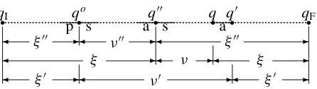
• Reverse ATTACH(cfr. (80, 90, 100)): ξ+= ξ0p andξ00+= ξ0νp/ν00. These formulas are made clear in Fig. 1.

• ReversePROJECT(cfr. (50, 60, 70)):ξ+=ξ0p.

• A reverse SHIFTis not necessary, but could be used as a computational check.

5_{Consequently the computation of LM probabilities}

re-quires almost no extra work. A model p(wj|q)used in (14) different from ps(wj|q)used by the parser may be chosen how-ever.

6_{Care has to be taken that an outer probability is complete}

qI

pq o

s aq

00

s qaq

0 _q

F

ξ00

ξ00

ν00

ξ

ξ

ν

ξ0

ξ0

ν0

Figure 1: Relations between inner and outer probabili-ties along a single path at attachment of q to q00resulting into q0.

Now the expected frequency of a transition o ∈ {s,p,a}from q to q0in a full parse of S is

E[Freq(q ⇒oq0|S)]= X

all paths

Pr(path|S)Freq(q ⇒oq0|path). (17)

Since all full parses terminate in qF, the final state,

ν(qF) = µ(qF) = Pr(S). Therefore (17) is

com-putable as

E[Freq(q ⇒oq0|S)]=

( ₁

ν(qF)ν(q

0_)ξ(q0_{) if o=s,}

1

ν(qF)ν(q)p(q⇒oq

0_)ξ(q0_{) else.} (18)

The expected frequencies required for the reesti-mation of the conditional distributions are then ob-tained by summing (18) over the state attributes from which the required distribution is independent.

4 Empirical evaluation

4.1 Modeling

We have trained two sets of models. The first set was trained on sections 0–20 of the Penn Treebank (PTB) (Marcus et al., 1995) using sections 21–22 for development decisions and tested on sections 23–24. The second set was trained on the BLLIP WSJ Corpus (BWC), which is a machine-parsed (Charniak, 2000) version of (a selection of) the ACL/DCI corpus, very similar to the selection made for the WSJ0/1 CSR corpus. As the training set, we used the BWC minus the WSJ0/1 “dfiles” and “efiles” intended for CSR development and evalua-tion testing.

The PTB devset was used for fixing submodel pa-rameterizations and software debugging, while per-plexities are measured on the PTB testset. The BWC trainset was used in rescoring N-best lists in order to assess the models’ potential in speech recognition. Both the PTB and BWC underwent

the following preprocessing steps: (a) A vocabu-lary was fixed as the 10k (PTB) resp. 30k (BWC) most frequent words; out-of-vocabulary words were replaced byhunki. Numbers in Arabic digits were replaced by one token ‘N’. (b) Punctuation was re-moved. (c) All characters were converted to lower-case. (d) All parse trees were binarized in much the same way as detailed in (Chelba, 2000, pp. 12–17); non-terminal unary productions were eliminated by collapsing two nodes connected by a unary branch to one node annotated with a combined label. This step allowed a simple implementation and compar-ison of results with related publications. We dis-tinguished 1891 different projections, 143 different non-terminal categories and 41 different parts-of-speech. (e) All constituents were annotated with a lexical head using deterministic rules by Magerman (1994).

The training then proceded by decomposing all parse trees into sequences ofSHIFT, PROJECT and ATTACH transitions. The submodels were finally estimated from smoothed relative counts of transi-tions using standard language modeling techniques: Good-Turing back-off (Katz, 1987) and deleted in-terpolation (Jelinek, 1997).

Shift submodel

The SHIFT submodel implements (40). Finding a good parameterization entails fixing the features that should explicitly appear in the context and in which order, so that all information-bearing ele-ments are incorporated, with limited data fragmen-tation. This is not a straightforward task. We went through an iterative process of intuitively guessing which feature should be added or removed from the context or changing the order, building a corre-sponding model and evaluating its conditional per-plexity (CPPL) against the devset. The CPPL of a SHIFT submodel is its perplexity measured on a test set consisting of (context, word to be pre-dicted) pairs (i.e. theSHIFTtransitions according to a certain parameterization) extracted from the cor-rect parse trees of a parsed test corpus. In other words, the CPPL is an underbound of the PPL in that it would be the PPL from an ideal parser. We fi-nally concluded that the parameterization (notation being consistent with (20))

ps(w|Y,x,L1.WORD), (19)

Table 1: Word trigram (baseline) and PTB model per-plexities.

model GT DI

(a) word trigram 190 193

(b) PLCG-based LM 185 187

(c) linear interpolation: .6(a) + .4(b) 159 166

this model on the PTB devset is 48, which displays the great potential of a correct syntactic partial parse to predict the next word.

Project/attach submodel

The ATTACH submodel can be incorporated into the PROJECT submodel by treating the attachment as a special kind of projection. This approach was systematically applied since it sped up pars-ing. Having the possibility to choose different pa-rameterizations in separate PROJECT and ATTACH submodels did not lower perplexity and increased execution time. Therefore, we always used com-bined PROJECT/ATTACH submodels in further ex-periments.

ThePROJECT/ATTACHsubmodel implements (70) and (100). The process of finding an appropriate parameterization used to build theSHIFTsubmodel was also applied here. Finally we concluded that the parameterization (notation being consistent with (50))

pp(T, α|Z,G,z) (20)

is optimal for our purposes in the given experimen-tal conditions.

4.2 Evaluation of PTB models

Table 1 lists test set perplexities (excluding OOVs and unparsed parts of sentences) of Good-Turing smoothed back-off models (GT) and deleted-interpolation smoothed (DI) models trained on the PTB trainset and tested on the PTB testset. We ob-served similar results with both smoothing meth-ods. As a baseline, word trigram (a) was trained and tested on the same material. The PPL obtained with the PLCG-based LM (b), using parametriza-tions (19) and (20), is not much lower than the base-line PPL.7_{Interpolation (c) with the baseline}

how-ever yields a relative PPL reduction of 14 to 16% with respect to the baseline.

7_{Using parametrizations p}

p(T, α|z,G,L1.CAT)for

projec-tion fromW-items and pp(T, α|G,Z,X,z)for other

projec-tions, we recently obtained a PPL of 178 (and 155 when inter-polated). This result is left out from the discussion in order to keep it clear and complete.

Table 2: WER results (%) after 100-best list rescoring on the DARPA WSJ Nov ’92 evaluation test set, non-verbalized punctuation. The models are smoothed with Good-Turing back-off (WER results in column GT) or deleted interpolation (DI).

rescoring model GT DI

(a) DARPA word trigram 10.44

(b) BWC word trigram 11.31 11.08

(c) BWC Chelba-Jelinek SLM 10.86

(d) (a) and (c) combined 9.82

(e) (b) and (c) combined 10.60

(f) BWC PLCG-based SLM 11.45 11.48

(g) (a) and (e) combined 9.85 9.87

(h) (b) and (e) combined 10.38 10.58

(i) Best possible 4.46 4.46

Parse accuracy is around 79% for both labeled precision and recall on section 23 of PTB (exclud-ing unparsed sentences, about 4% of all sentences). In comparison, with our own implementation of Chelba-Jelinek, we measured a labeled precision and recall of 57% and 75% on the same input. These results seem fairly low compared to other recent work on large-scale parsing, but may be partly due to the left-to-right restriction of our language mod-els,8 which for instance prohibits word-lookahead. Moreover, while we measured accuracy against a binarized version of PTB, the original parses are rather flat, which may allow higher accuracies.

4.3 Evaluation of BWC-models

The main target application of our research into LM is speech recognition. We performed N-best list rescoring experiments on the DARPA WSJ Nov ’92 evaluation test set, non-verbalized punctuation. The N-best lists were obtained from the L&H Voice Xpress v4 speech recognizer using the standard tri-gram model included in the test suite (20k open vo-cabulary, no punctuation).

In Table 2 we report word-recognition error rates (WER) after rescoring using Chelba-Jelinek and PLCG-based models. Both DI and GT smooth-ing methods yielded very comparable results. Due to technical limitations, all the models except the baseline trigram were trimmed by ignoring highest-order events that occurred only once.

The best PLCG-based SLM trained on the BWC train set (f) performs worse than the official word trigram (a). However, since the BWC does not com-pletely cover the complete WSJ0 LM train material

and slightly differs in tokenization, it is more fair to compare with the performance of a word trigram trained on the BWC train set (b). Results (g) and (h) show that the PLCG-based SLM lowers WER with 4% relative when used in combination with the baseline models. A comparable result was obtained with the Chelba-Jelinek SLM (results (d) and (e)).

5 Conclusion and future work

The PLCG-based SLM exposes a slight loss of ro-bustness in the reduced recognition rate when it is used as a stand-alone rescoring LM. Combined with a word trigram LM however, perplexity and WER reductions with respect to a word 3-gram baseline seem similar to those obtained with the Chelba-Jelinek SLM and those previously reported by Chelba (2000). On the other hand, the PLCG-based SLM is significantly faster and obtains a higher parsing accuracy.

In the future we plan to evaluate full EM reesti-mation of the models on the trainset using the for-mulas given in this paper.

Acknowledgements

The authors wish to thank Paul Vozila for discussing intermediate results and for providing the authors with the 100-best lists used for sentence rescoring. The authors are also indebted to Saskia Janssens and Kristin Daneels for their help with some of the ex-periments.

This research is supported by the Institute for the promotion of Innovation by Science and Tech-nology in Flanders (IWT-Flanders), contract no. 000286.

References

James K. Baker. 1979. Trainable grammars for speech recognition. In Jared J. Wolf and Den-nis H. Klatt, editors, Speech Communication Pa-pers for the 97th Meeting of the Acoustical Soci-ety of America, pages 547–550. The MIT Press, Cambridge, MA.

Eugene Charniak. 2000. A maximum-entropy in-spired parser. In Proc. of the NAACL, pages 132– 139.

Ciprian Chelba. 2000. Exploiting Syntactic Struc-ture for Natural Language Modeling. Ph.D. the-sis, Johns Hopkins University.

Michael J. Collins. 1996. A new statistical parser based on bigram lexical dependencies. In Proc.

of the 34th Annual Meeting of the ACL, pages 184–191.

Frederick Jelinek and Ciprian Chelba. 1999. Putting language into language modeling. In Proc. of Eurospeech ’99, volume I, pages KN– 1–6.

Frederik Jelinek and John Lafferty. 1991. Compu-tation of the probability of initial substring gener-ation by stochastic context-free grammars. Com-putational Linguistics, 17(3):315–323.

Frederick Jelinek. 1997. Statistical Methods for Speech Recognition. The MIT Press, Cambridge, MA.

Slava M. Katz. 1987. Estimation of probabili-ties from sparse data for the language model component of a speech recognizer. IEEE Trans. on Acoustics, Speech and Signal Processing, 35:400–401.

David M. Magerman. 1994. Natural Language Parsing as Statistical Pattern Recognition. Ph.D. thesis, Stanford University.

Christopher D. Manning and Bob Carpenter. 1997. Probabilistic parsing using left corner language models. In Proc. of the Fifth International Work-shop on Parsing Technologies, pages 147–158. Christopher D. Manning and Hinrich Sch¨utze.

1999. Foundations of Statistical Natural Lan-guage Processing. The MIT Press, Cambridge, MA.

Mitchell P. Marcus, Beatrice Santorini, and Mary Ann Marcinkiewicz. 1995. Building a large annotated corpus of English: the Penn Tree-bank. Computational Linguistics, 19(2):313– 330.

Brian Roark and Mark Johnson. 2000. Efficient probabilistic top-down and left-corner parsing. In Proc. of the 37th Annual Meeting of the ACL, pages 421–428.

Andreas Stolcke. 1995. An efficient probabilis-tic context-free parsing algorithm that computes prefix probabilities. Computational Linguistics, 21(2):165–201.

Filip Van Aelten and Marc Hogenhout. 2000. Inside-outside reestimation of Chelba-Jelinek models. Internal Report L&H–SR–00–027, Lernout & Hauspie, Wemmel, Belgium.