575
Modeling Confidence in Sequence-to-Sequence Models
Jan Niehues
Department of Data Science and Knowledge Engineering (DKE)
Maastricht University
Ngoc-Quan Pham Institute of Anthropomatics Karlsruhe Initute of Technology
Abstract
Recently, significant improvements have been achieved in various natural language process-ing tasks usprocess-ing neural sequence-to-sequence models. While aiming for the best generation quality is important, ultimately it is also nec-essary to develop models that can assess the quality of their output.
In this work, we propose to use the similarity between training and test conditions as a mea-sure for models’ confidence. We investigate methods solely using the similarity as well as methods combining it with the posterior prob-ability. While traditionally only target tokens are annotated with confidence measures, we also investigate methods to annotate source to-kens with confidence. By learning an inter-nal alignment model, we can significantly im-prove confidence projection over using state-of-the-art external alignment tools. We eval-uate the proposed methods on downstream confidence estimation for machine translation (MT). We show improvements on segment-level confidence estimation as well as on con-fidence estimation for source tokens. In addi-tion, we show that the same methods can also be applied to other tasks using sequence-to-sequence models. On the automatic speech recognition (ASR) task, we are able to find 60% of the errors by looking at 20% of the data.
1 Introduction
Deep learning methods have significantly in-creased the quality of natural language generation tasks such as Machine Translation (MT). How-ever, when deployed in a production environment, understanding the model’s confidence and how well it correlates with output quality is as impor-tant as training the best models.
While humans are often capable of estimating whether their decisions are sensible or produced
by random guesses, it is often not possible to know how confident deep learning models are with re-spect to their output (Gal, 2016). However, in-formation regarding confidence can be essential in production scenarios. In cases with a human-in-the-loop, confidence can be used to identify the parts of the machine output that require human in-tervention, e.g. in post-editing for machine trans-lation or to guide reformutrans-lation of the original in-put to simplify the task for sequence-to-sequence models.
Intuitively, models should have higher confi-dence towards data points that are similar to their training data. Motivated by this, our first contribu-tion is an autoencoder network that is applied as an extension to the sequence-to-sequence models to measure the training-testing discrepancy. In con-trast to methods that directly compare the test and training data to generate confidence scores, we do not need to store the whole training data, thereby enabling our method to scale to larger datasets and tasks.
Motivated by the successful application of pos-terior probabilities for confidence estimation in statistical machine translation (SMT) (Ueffing and Ney,2007) and traditional ASR systems (Siu and Gish,1999), our second contribution is a combi-nation our approach with this prior approach.
tokens in complex sequence-to-sequence models. We can show that this strongly outperforms exter-nal state-of-the-art alignment methods.
Our experiments shows that in machine transla-tion, the posterior probabilities can be competitive with automatic metrics in terms of correlation with human evaluation. For speech recognition, we are able to find 60% of the errors by looking at 20% of the data.
2 Confidence Estimation Task
Depending on the use case, there are different ways to define the task of confidence estimation. Furthermore, there is no clear separation between confidence estimation and quality estimation. A first important dimension is the granularity of the predictions. We investigate three different use cases in this work, described in the next three sub-sections in greater detail.
Previous methods differ in whether they pre-dicting continuous values or discrete labels. In this work, we will predict continuous values, but eval-uate against gold standard labels. In Section5, we describe in detail how we map continuous predic-tions to discrete labels.
In addition, previous methods differ in whether they can be trained on gold standard labels or if no annotated training data is available. Training data is a particular challenge in confidence estimation since annotations are associated with the output of a particular model. Therefore, this raises the ques-tion whether the task is to estimate the quality of any model, or of a particular one. This has im-plications for whether we can use model internal information or not. In this work, we focus on the situation where we want to estimate the confidence of a particular model, using internal information. Since in a realistic real-world scenario we are not able to collect annotated data for each model we are interested in, we further do not use any labeled training data.
2.1 Granularity
First, the confidence of the whole output sequence can be estimated. Given an input sequenceX =
x1. . . xIwand an output sequenceY =y1. . . yJw,
the model estimates quality c for the whole se-quence. We will present several methods that calculate a sequence of confidence estimations
c01, ..., c0L. Therefore, we need an additional ag-gregation function for the sequence confidence
es-timates. In all our experiments, we are using the minimum as the aggregation function.
In some use cases, it is important to get more fine-grained quality estimation. To be specific, we aim at estimating the confidence of every target token xj instead of one single score for the
se-quence. Given an input sequenceX =x1. . . xIw
and an output sequenceY = y1. . . yJw, the
out-put will be a sequence of quality estimationsC =
c1. . . cJw. One additional challenge is that we
might be interested in the confidence using a dif-ferent granularity than the predicted by the model
c01, ..., c0L (withL 6= Jw). For example, the user
is interested in word-based confidence, while the system uses subword units. In this case, we as-sume to have a mappingmbetween the positions 1. . . Jw and1. . . L. In the example of subwords,
this is straightforward because segmentation is re-coverable. Then, we also need an additional ag-gregation function for the confidence estimates. We estimate the confidencecj by aggm(l)=j(cl).
For this type of aggregation we also use the mini-mum.
In machine translation, it is not only the con-fidence at the output level that is of interest, but also how adequately each individual source token is translated. From an application point of view, when the machine translation is used in an inter-active scenario, this feature for example enables the user to reformulate the source sentence in or-der to avoid phrases that the system is not able to handle.
Formally, given an input sequence X =
x1. . . xIwand an output sequenceY =y1. . . yJw,
the model estimates a sequence of confidence measuresC = c1. . . cIw. Therefore, in this case,
given the estimation of the model c01, ..., c0L, we need a mappingmbetween the positions1. . . Iw
and1. . . L.
2.2 Posterior Probabilities
As a baseline for our experiments, we use the pos-terior probabilities. The intuition behind this tech-nique is that the model will distribute the proba-bility mass over several outputs in low-confidence situations. In contrast, if the model is confident about its prediction, it should assign a high proba-bility to the prediction.
Formally, given an input sequence X =
x1. . . xIwand an output sequenceY =y1. . . yJw,
and an output sequence Y0 = y10 . . . y0J
t (e.g. by
using subwords). The encoder will first calculate a sequence of hidden states E = e1, . . . eIt =
EN C(X0). Secondly, we predict the target hid-den states D = d1, . . . dJt = DEC(E, Y
0).
Fi-nally, we can use the posterior probabilitiesP =
p1, . . . , pJt calculated by:
pi =sof tmax(F F(di))[y0i] (1)
whereF F is a linear transformation and[k] indi-cates thek-th element of the vector. By using P
forC0 as described in Section 2.1, we can calcu-late now a sequence confidence or an output con-fidence.
3 Training similarity
The similarity between test input and the examples seen in training is an important indication for the model’s performance. Intuitively, models should be better at predicting examples similar to their training data than examples very different from the training data.
3.1 Approaches to measure similarity
Two sentences can be similar in many ways. Therefore, there are also many ways to estimate the similarity between sentences. For our use case, it is important how similar the sentence repre-sentation generated by the translation systems is. Hence, we use the internal representations of the neural machine translation model to measure the similarity of the sentences.
In an NMT system, there are different represen-tation levels which can be used to measure the sim-ilarity of the sentence. For example, we can use the final encoder hidden states, the final decoder hidden states, or the context vectors. As motivated in the introduction, one interesting use case for us-ing confidence is to find difficult source segments, so that the user can rewrite them. For this case, we concentrate on the encoder hidden states.
We measure the training-test similarity as fol-lows: First, we run the encoder on the source side of the training data and store the encoder hidden representation (top layer) for every sen-tence k (Ek = ek
1, . . . , ekIk
t). Second, we
cal-culate the hidden representations of the test sen-tences (Etst = etst1 , . . . , etstItst
T
) and used approx-imate k-nearest neighbor search (implemented in
the Annoy1toolkit).
We investigated two methods to estimate the similarity, one on the sentence level and one on token level. First, we use the distance to the over-all most similar training sentence by using the av-erage vector of the encoder hidden states for the training as well as for the test data. Formally:
s= min
k∈trainL
2(avg(ek
1, . . . , ekIk), avg(e
tst
1 , . . . , etstItst))
(2) Then we usesdirectly as the sequence confidence
cfrom Section 2.1.
The second method is to estimate the confidence for each source token. This is achieved by finding the nearest neighbor for each hidden encoder state
etsti .
si min
k∈train;ik∈1,...,Ik
L2(eki
k, e
tst
i ) (3)
By usingS =s1. . . sItst asC0 in Section 2.1, we
can calculate a sequence confidence or an confi-dence for each input token.
3.2 Similarity estimation
The main disadvantage of aforementioned method is that we need to calculate and store the hid-den representation of all training examples. Such storage consumption is non-trivial even for small datasets like the TED corpus and it is infeasible for large-scale sequence-to-sequence models.
Therefore, we also investigate methods to ap-proximate the distance without storing the hidden states for the whole training data. Here we pro-pose to approximate this distance by using au-toencoders. The autoencoder will be able to re-construct typical hidden states seen in the training data, while the reconstruction of unusual hidden states will be less exact.
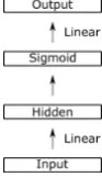
As shown in Figure 1, we are using an autoen-coder with a single hidden layer. In our experi-ments, we investigate different hidden sizes of the autoencoder. Afterwards, we apply the sigmoid activation function before predicting the output.
Next, we then can use the quality of the recon-struction as a measure of the model’s confidence in its predictions. We found that it is possible to get the confidence qualitatively by measuring theL2 -distance between the hidden representation and its reconstruction.
sei =L2(ei, Auto(ei)) (4)
As for the direct measurement, we can useSe =
se1. . . seItst asC0 to calculate the confidence of the
[image:4.595.157.204.168.249.2]sequence or for each input token. Furthermore, by using the decoder statesDinstead of the encoder statesE, we can calculateSdaccordingly and use it to estimate the sequence or target token confi-dence.
Figure 1: Architecture of the autoencoder
3.3 Combining both approaches
While using similarity measurements is able to es-timate the quality of the whole sequence as well as of parts of the sequence, it also has two draw-backs: First, in the L2-norm all dimensions are equally important, while this might not be the case for the final prediction of the words. Second, we are only looking at the similarity between training and test condition, but ignoring that some outputs might be inherently more difficult to predict than others.
Therefore, we combine both techniques and thereby minimize their respective drawbacks. To do so, the hidden representation is first replaced by the reconstruction generated by the autoencoder. After that, we calculate the probabilities based on these reconstructed hidden representations. If we use the autoencoder on the decoder states, Equa-tion1needs to be modified to:
psi =sof tmax(F F(Auto(di)))[y0i] (5)
By using Ps for C as described in Section 2.1, we can calculate now a sequence confidence or an output confidence. Similarly, we can replace
Auto(di) by d0i withD0 = DEC(Auto(E), Y0)
to use the autoencoders on the encoder hidden states. It is important to note, that the similarity approximated by the encoder hidden states can be used for source token confidence estimation, while the combination of autoencoders on the source hidden state and posterior probabilities can only be used for target token confidence estimation. One advantage of this combination is that no additional parameters are introduced.
4 Alignment
While the previously presented models are all able to generate confidence measures for each target to-ken, only the distance-based similarity measures are able to also generate scores for the source to-kens. In order to generate source token confidence qualitatively, a straightforward approach is to use word alignment to map the confidence score from the target side to the source.
Our baseline for these experiments uses the IBM4 GIZA alignment model (Och and Ney,
2003) to map the posterior probabilities and the combined approach’s confidence estimations from target to source tokens. If several target tokens align to the same source token, we again use the minimal confidence.
Motivated by our autoencoding approach to measure similarity between training and test data, we investigate similar approaches to model the alignment between source and target tokens. In this case, we used a model to predict a target hid-den state dj given a source state ei. If a source
word aligns to a target word, it should be possi-ble to predict this target word primarily based on this source word. Therefore, we choose the same architecture as for the autoencoder. We use the source hidden state to predict a target hidden state. Then, we compare the predicted hidden state to all decoder hidden states and describe the align-ment strength between the source and target hid-den state using the cosine similarity between the predicted hidden state and the target hidden state. LetN N()be the neural network-based predictor. We then calculate the alignment by:
a0ij = cossim(N N(ei), dj) (6)
Based on the alignment scores, we created an alignment matrix by aligning each source word to the target word with the strongest link according to Equation7.
a(i) = min
j∈1,...,Ja 0
ij (7)
Since there are not confidence labels with aligned source and target words available, we can-not simply train the neural network. Inspired by the GIZA model, we utilize the EM algorithm for training. Given an alignmenta∗, we can train our model using the following MSE-based loss func-tion:
This can be extended for soft alignmentsato:
M SE(N N(ei),
X
j
aijdj) (9)
This corresponds to the M-Step in the EM algo-rithm. To be able to train the model using this loss function, we need to estimate an alignmentain the E-step. Given the source representatione1, . . . eI
of a sentence, we use the predictor to calculate the prediction p1, . . . pI. Based on this, we calculate
the alignment similaritiesa0ijbased on cosine sim-ilarities betweenpi and the decoder hidden states dj. In order to prevent the model from learning to
collapse into aligning all source words to the most obvious words e.g. the period at the end of the sen-tence, we normalize them to probabilities for each target word. (a0ij =aij/PiI0=1(ai0j)).
5 Evaluation
In this work, we evaluate the ability of sequence-to-sequence models to estimate their confidence in their own output on two different tasks: MT and ASR.
It is necessary to define a gold standard for the evaluation. For ASR, there is only one ground truth. Accordingly, we can la-bel each output word from the model as cor-rect/substitution/deletion/insertion. Our confi-dence measurement is then done on he word level (predicting whether the word is correct or not)2.
For machine translation, a single correct trans-lation for each source sentence does not exist. To account for this, our experiments are carried out in the following way: We collected annotations with incorrectly translated source words for 1177 sen-tence pairs, resulting in39.93%of the source sen-tences containing mistranslated words. We were not able to test our methods on existing quality estimation data sets, as we cannot access internal model information for this data.
Given the reference labels, the next step is to measure the quality of the confidence measures. In our experiments, we use four different measures. The first possible scenario is that, we assume that the user has a fixed amount of time and wants to maximize the improvements. Therefore, we cal-culate the confidence score for all the test data and look at the 10% and 20% of the test data that the model has given the lowest confidences. Then,
2If a word in the reference was deleted, we marked the
previous and next word also as an erroneous word.
we measure what percentage of errors according to the reference are found in this part of the data.
In another scenario, we want to dynamically correct as many sentences as would be beneficial. This can be measured using the F-Score. Since we need to map the confidence scores to labels, we have the additional challenge of finding a good threshold for when to assign the label “high con-fidence” or “low concon-fidence” to an output sen-tence/word. Therefore, we report oracle F-Scores using an optimal threshold found on the test data. Furthermore, we evaluate an approach to find this threshold in an unsupervised manner: While our baseline system uses beam search with beam=8, we also perform greedy decoding. We assume that the model is not confident if the beam search leads to a different outcome from the greedy decod-ing, and create pseudo-labels where each segment or token is labeled wrong if the results of beam search and greedy search differ. Then, we select the optimal threshold based by comparing the pre-dict scores and these pseudo-labels and evaluate the approach on the real labels.
6 Experiments
The sequence-to-sequence models in our work are based on the state-of-the-art Transformer architec-ture (Vaswani et al.,2017). We followed the model configuration with the learning rate schedule from theBase configuration in the original work. The number of layers is adapted for each task for the best performance possible and will be reported respectively. The autoencoders are implemented on top of the Transformer (with PyTorch (Paszke et al., 2017)) using one hidden layer with differ-ent sizes and sigmoid activation function. 3 The MT model is a 12-layer Transformer trained on the German-English TED corpus (Cettolo et al.,
2012) with the development set and test set from the IWSLT 2017 evaluation campaign. The data is preprocessed with Moses tokenization, true-casing and segmented with byte-pair encoding (Sennrich et al.,2016) with 40K codes. The model achieves a BLEU score of28.82on the development set and 30.63on the test data.
We conducted further ASR experiments on the Switchboard-1 Release 2 (LDC97S62) corpus, which contains over 300 hours of speech. The Hub5’00 evaluation data (LDC2002S09) was used as our test set. On this set, we are especially
ested in the influence of the model performance on the quality estimation. Therefore, we trained 4 different models with 4,8,12 and 24 layers. These models achieve a WER of 20.8, 14.8, 13.0 and 12.1on the Switchboard test set respectively, and 33.2,25.5,23.9and23.0on the Callhome set.
6.1 Machine translation results
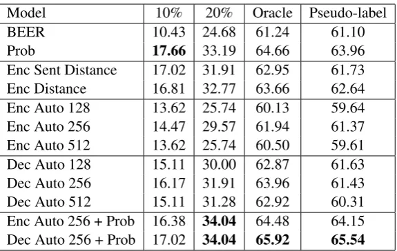
The first concern in the experiments is the perfor-mance on segment-level quality estimation for ma-chine translation. The results are summarized in Table1.
Two baseline systems are presented in this ex-periment. To measure the difficulty of the task, we use the BEER evaluation metric as comparison, which has been performing competitively in the WMT Metric evaluations (Stanojevic and Simaan,
2014). It is important to note that the metric has access to the reference translation, while the con-fidence measure do not. Even with this advantage, the metric does not clearly outperform a random baseline, showing the difficulty of the task. Using the model’s posterior probability, we can improve on all four types of confidence measure. Among the 10% of the sentences with the lowest confi-dence, this method was able to find 17.66% of the sentences with errors. For this task, this is further the best performance. This confirms our hypoth-esis that the posterior probabilities can be reliable for modelling the system’s confidence.
Proceeding to experiments shown in the next two lines, we evaluate the ability of using the sim-ilarity between test and training data as a measure for confidence. Although not performing as well as the posterior probabilities, the data difference is a good estimator for the task difficulty and the con-fidence of the model. When comparing a single sentence representation (Enc Sent Distance) and the token representation (Enc Distance) in the next line, the second one outperforms the first one, ex-cept for the top 10%. Therefore, it seems to be important to measure the distance of each individ-ual token and not only of the whole sentence.
Motivated by these results, we trained the au-toencoders on the individual tokens and not on the whole sentence and used the autoencoder net-works on the source hidden representation to esti-mate the performance. We analyze the influence of the size of the bottleneck of the autoencoder. The network with bottleneck size of 256 (Enc Auto 256), which is half the size of the input size,
man-aged to get the best performance in all measures. While we see a drop in performance due to the ap-proximation, e.g. from 32.77% to 29.57% when looking at 20% of the data, this is still better than BEER.
We performed the same experiment using the target hidden representations. Again, we inves-tigated the influence of the bottleneck size and achieved the best performance with a bottleneck size of256(Dec Auto 256). Reasonably, the target hidden states contain more information about the sequence-to-be-generated than the source states.
Finally, when combining the output probability with the decoder hidden states (Dec Auto 256 + Prob), we are able to achieve the best performance. Again, it is better to use the autoencoder on the decoder hidden state than on the encoder hidden state. It is worth noting that the pseudo-labels per-form very well when including the posterior prob-abilities. Interestingly, we see a clear drop in per-formance between oracle and pseudo-labels when not using the posterior probabilities.
Moreover, we evaluated methods to identify source words with low confidence. The results for these experiments are summarized in Table2. In this case the baseline is to map the posterior prob-abilities to the source sentence using a GIZA (Och and Ney,2003) alignment. Again, we evaluate the approach with the same four scores. As shown in the first two lines, the Giza alignment from source to target performance clearly better than the one from target to source. Therefore, in the remaining experiments, we only evaluate approaches using the source to target alignment.
Model 10% 20% Oracle Pseudo-label
BEER 10.43 24.68 61.24 61.10
Prob 17.66 33.19 64.66 63.96
[image:7.595.156.444.60.242.2]Enc Sent Distance 17.02 31.91 62.95 61.73 Enc Distance 16.81 32.77 63.66 62.64 Enc Auto 128 13.62 25.74 60.13 59.64 Enc Auto 256 14.47 29.57 61.94 61.37 Enc Auto 512 13.62 25.74 60.50 59.61 Dec Auto 128 15.11 30.00 62.87 61.63 Dec Auto 256 16.17 31.91 63.96 61.43 Dec Auto 512 15.11 31.28 62.92 60.31 Enc Auto 256 + Prob 16.38 34.04 64.48 64.15 Dec Auto 256 + Prob 17.02 34.04 65.92 65.54
Table 1: Segment-level confidence estimation for MT. First two columns: Percentage of found errors when select-ing 10% and 20% of the data; Final two columns: F-score when usselect-ing oracle threshold and thresholds optimized on pseudo-labels
Model Alignment 10% 20% Oracle Pseudo-label Prob Giza DE-EN 25.15 34.09 19.33 17.73 Prob Giza EN-DE 28.90 39.86 22.58 21.18
Enc Auto 256 28.78 49.58 23.54 16.31
Dec Auto 256 Giza EN-DE 32.21 49.51 24.85 19.49 Enc Auto 256 + Prob Giza EN-DE 29.75 40.44 22.97 22.37 Dec Auto 256 + Prob Giza EN-DE 32.21 47.38 24.54 24.37
Prob 256 32.34 44.59 25.16 24.25
Prob 512 32.79 44.91 25.45 24.39
Prob 2048 32.27 44.91 24.98 23.85
Prob 8192 33.38 46.34 25.63 24.33
Dec Auto 256 8192 33.89 53.27 26.23 21.65 Dec Auto 256 + Prob 8192 35.58 52.62 27.21 27.02
Table 2: Source word confidence for MT. First two columns: Percentage of found errors when selecting 10% and 20% of the data; Final two columns: F-score when using oracle threshold and thresholds optimized on pseudo-labels
posterior probabilities when looking at 10% and 20% of the data. Finally, we tried to use an internal alignment instead of the Giza alignment. There-fore, we predict the decoder hidden states based on the encoder hidden states as described in Section
4. Again, we investigated different sizes for the hidden states used to map the posterior probabili-ties. As shown in Table2, all the models perform better than the GIZA alignment. We can further improve the quality by using a larger hidden layer. Since we need to learn a very complex mapping from source to target hidden states, a larger layer is better. The best performance is achieved using a layer of 8192 hidden units.
In the end, we also used the same model to map
the autoencoder predictions. The combination of all three methods leads to the best results (Dec Auto 256 + Prob, 8192). By looking only at 10% of the words, we are able to find more than 35% of the errors and for 20% of the words we identify more than half of the errors.
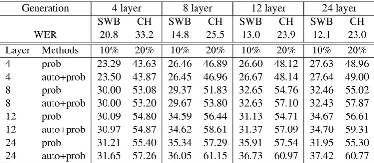
6.2 Speech recognition results
Generation 4 layer 8 layer 12 layer 24 layer
SWB CH SWB CH SWB CH SWB CH
[image:8.595.106.491.61.229.2]WER 20.8 33.2 14.8 25.5 13.0 23.9 12.1 23.0 Layer Methods 10% 20% 10% 20% 10% 20% 10% 20% 4 prob 23.29 43.63 26.46 46.89 26.60 48.12 27.63 48.96 4 auto+prob 23.50 43.87 26.45 46.96 26.67 48.14 27.64 49.00 8 prob 30.00 53.08 29.37 51.83 32.65 54.76 32.46 55.02 8 auto+prob 30.00 53.20 29.67 53.80 32.63 57.10 32.43 57.87 12 prob 30.09 54.80 34.59 56.44 31.13 54.71 34.67 56.61 12 auto+prob 30.97 54.87 34.62 58.61 31.37 57.09 34.70 59.31 24 prob 31.21 55.40 35.34 57.29 35.91 57.54 31.95 55.30 24 auto+prob 31.65 57.26 36.05 61.15 36.73 60.97 37.42 60.77
Table 3: Confidence estimation on ASR using different ASR systems for output predictions and confidence esti-mation: Found errors when selection 10% and 20% of the data
Here we evaluated four different models with increasing transcription quality. The only differ-ence between the models are the number of hidden layers. We investigated models using4,8,12and 24layers. In this task, the test set consists of two subsets. The best model achieves a word error rate of12.1and23.0on the two subsets, respectively.
Again, we use the output probabilities as well as the combination of the autoencoder and the output probabilities. We again use half the input size for the bottleneck size. Firstly, as shown in the MT experiments, we can improve the quality estima-tion by combining the posterior probabilities and the autoencoder approach. In all configurations, the combination performs better or similar than the posterior probability.
Secondly, the better models are able to better es-timate the confidence on the same output. In most cases, the performance can be improved by using a more complex model to estimate the confidence. One exception is the estimation of its own output. Finally, the estimation of the distance between training and test data mainly helps when using stronger models, both for the generation of the out-put and for confidence estimation. Furthermore, this method also removes the effect of models per-forming worse than their own output.
7 Related Work
Prior work has investigated confidence measure-ment for speech recognition models (Siu and Gish,
1999), and statistical machine translation mod-els using either word-level posteriors (Ueffing and Ney, 2007) or external models (Gandrabur and Foster, 2003). Deep learning models have
also received attention on uncertainty and confi-dence measurement recently: (Gal and Ghahra-mani, 2016) formulate neural network models with dropout as Bayesian models to obtain uncer-tainty based on sampling methods. Specifically, for neural machine translation models or other sequence-to-sequence models, quality estimation has remained as a topic of concern. While most prior research focused on developing confidence measures for a general system using external fea-tures (Specia et al.,2018), this works concentrates on estimating the confidence of a specific system by making use of the information available in the internal representation of the network.
8 Conclusion
In this work, we investigated the ability of sequence-to-sequence models to model their con-fidence in their decisions. We performed experi-ments using these models for two tasks: machine translation and speech recognition.
We analyzed the influence of train-test mis-match on quality estimation. By approximating this mismatch using an autoencoder and combin-ing it with the posterior probabilities, we are able to improve confidence estimation over a strong baseline. We showed that it is better to measure the mismatch on the decoder hidden states than on the encoder hidden states.
sequence-to-sequence models. Using this alignment instead of a state-of-the-art external alignment for mapping target confidence measure to source tokens clearly improved the quality of the confidence measure for source words
Acknowledgments
The project ELITR leading to this publication has received funding from the European Unions Hori-zon 2020 Research and Innovation Programme un-der grant agreement No825460. We thank Eliza-beth Salesky for the constructive comments.
References
Mauro Cettolo, Christian Girardi, and Marcello Fed-erico. 2012. Wit3: Web inventory of transcribed and
translated talks. In Proceedings of the 16th Con-ference of the European Association for Machine Translation (EAMT), pages 261–268, Trento, Italy.
Yarin Gal. 2016.Uncertainty in Deep Learning. Ph.D. thesis, University of Cambridge.
Yarin Gal and Zoubin Ghahramani. 2016. A theoret-ically grounded application of dropout in recurrent neural networks. InAdvances in Neural Information Processing Systems 29 (NIPS).
S. Gandrabur and G. Foster. 2003. Confidence estima-tion for translaestima-tion predicestima-tion. InProceedings of the Seventh Conference on Natural Language Learn-ing at HLT-NAACL 2003 - Volume 4, CONLL ’03, pages 95–102, Stroudsburg, PA, USA. Association for Computational Linguistics.
Franz Josef Och and Hermann Ney. 2003. A System-atic Comparison of Various Statistical Alignment Models.Computational Linguistics, 29(1):19–51.
Adam Paszke, Sam Gross, Soumith Chintala, Gre-gory Chanan, Edward Yang, Zachary DeVito, Zem-ing Lin, Alban Desmaison, Luca Antiga, and Adam Lerer. 2017. Automatic differentiation in pytorch.
Rico Sennrich, Barry Haddow, and Alexandra Birch. 2016. Neural machine translation of rare words with subword units. Proceedings of the 54th An-nual Meeting of the Association for Computational Linguistics (Volume 1: Long Papers).
M. Siu and H. Gish. 1999. Evaluation of word con-fidence for speech recognition systems. Computer Speech & Language, 13(4):299 – 319.
L. Specia, F. Blain, V. Logacheva, R. Astudillo, and A. F. T. Martins. 2018. Findings of the wmt 2018 shared task on quality estimation. InProceedings of the Third Conference on Machine Translation, Vol-ume 2: Shared Task Papers, pages 702–722, Bel-gium, Brussels. Association for Computational Lin-guistics.
Milos Stanojevic and Khalil Simaan. 2014. Beer: Bet-ter evaluation as ranking. In Proceedings of the Ninth Workshop on Statistical Machine Translation, pages 414–419.
N. Ueffing and H. Ney. 2007. Word-level confidence estimation for machine translation. Computational Linguistics, 33:9–40.