New studies on network frequency responses considering dynamic loads

Vol.08, No.03, December 2019, pp. 01-11

ISSN: 2252-8792  1

Journal homepage: http://iaescore.com/journals/index.php/IJAPE

New Studies on Network Frequency Responses Considering

Dynamic Loads

L.T.M. Trang1_{, H. Nouri}2

1_{Department of Instrumentation and Control Engineering, CTU in Prague, CZ} 2_{Power System, Electronics and Control Research Laboratory, UWE in Bristol, UK}

Article Info ABSTRACT

Article history:

Received Dec, 2018 Revised Jan, 2019 Accepted …..., 2019

The dynamic model construction of transmission network components that include generator buses, load buses and power branches, within MATLAB-Simulink environment is presented. The degree of frequency deviation of buses when the power of motor loads and static loads vary, is studied. Furthermore, the influence of motor loads with different inertia constants are considered in the control technique of load frequency using a PID controller. The results show that the frequency oscillation of the dynamic load is greater than the frequency oscillation of static load. Also the speed of frequency control of the dynamic load is greater than the speed of the frequency control of the static load and the inertia constants of the dynamic load has significant influence on the frequency control characteristics.

Keywords:

Automatic Generation Control (AGC)

Induction Motor (IM)

Load Frequency Control (LFC)

Optimal Load Control (OLC)

Area Control Error (ACE) Copyright © 2018 Institute of Advanced Engineering and Science. All rights reserved.

Corresponding Author:

L.T.M. Trang

Department of Instrumentation and Control Engineering, Czech Technical University in Prague,

Technical 4, Praha 6, 16607, Czech Republic Email: [email protected]

1. INTRODUCTION

In recent years, the increasing stress in a transmission system may limit the effective power transfer from generation to the load. At steady state, the frequencies on different buses in a system are synchronized to a common nominal value and the mechanical power is balanced with the electrical power on each bus. Suppose a small change in power balance injection occurs on an arbitrary bus. This mismatch between generation and load causes the bus frequency to deviate from its nominal value. Consequently, the system may lose stability and cause damage to the facilities if the frequency deviations are not tightly controlled around zero. This is important as the frequency of a power system is an indispensable performance signal to the system operator for security and stability considerations. Hence, the desired power system frequency should be kept within a very small, acceptable margin around its nominal value. Otherwise, the system operator must take relevant and effective actions immediately to avoid physical damage to devices.

A power system is a combination of generation, transmission, distribution networks and loads. The active and reactive power demands from different loads vary continuously. The induction motors account for a large portion of electrical loads in industry and air conditioning in business and residential areas. Dynamic characteristics of these loads affect the response of system stability when compared to static loads. Hence, the influence of motors as dynamic loads on transient stability studies have attracted a great deal of attention. The linearized models of dynamic loads [1][2][19] and load frequency control strategies [3] on a nonlinear system are considered to develop a robust controller.

In an interconnected system, as a power load demand varies randomly, both bus frequency and line power interchange will also vary. The objectives of Load Frequency Control (LFC) are to minimize the transient deviations in these variables (bus frequency and line power interchange) and to ensure their steady state error to be close to zero. Thus, a control system is essential to overcome the effects of the random load changes and to keep the bus frequency within the range of nominal value.

In the past decades, many researchers have investigated the power network frequency regulation. Since the system frequency is essentially related to real power balance, it is natural to control real power output in the generation side through the use of automatic generation control (AGC) system [5] – [8].

There are some simulation studies of frequency load control in a single area of power network which include one generator or several generators in parallel operation [9][10]. However, for large scale power systems which consist of interconnected control areas, it is important to keep the frequency constant and the tie line power near to its scheduled value. This is achieved by implementing LFC as Tie line controller and PID controller [6][7]. There are much more analytic studies that relate the behavior of the loads and frequency responses of interconnected power network [11]-[13]. This is normally achieved through establishment of the well-known generation swing equation and implementation of classic tools such as transfer function [11][12] and state space method [14] in the swing equation to estimate the amount of frequency deviation.

With the above motivations, this paper contributes initially to the construction of a dynamic model of a transmission network including generator buses, load buses and power branches within MATLAB-Simulink environment. Then investigates the degree of frequency deviation of buses when power of motor loads and static loads vary. In addition, the influence of motor loads with different inertia constants are considered in the control technique of load frequency using a PID controller.

The remaining parts of this paper are organized as follows: mathematical modelling of a dynamic system are shown in Section 2; the proposed controller of load frequency and influence of motor load to control quality are presented in Section 3; the simulation results are given in Section 4; and the concluding remarks are given in Section 5.

2. NETWORK MODEL DEVELOPMENT

In the interconnected network, buses could possess generators, loads or neither. A generator bus not only has an AC generator that converts mechanical power into electrical power through a rotating prime mover, but some loads may also be attached to it. However, on the load bus, only loads are connected to the load bus. To construct the dynamic model of a network, the description model of a Turbine-Generation system needs to be developed. Then the models of power equilibrium equation for the generation bus, load bus and power branch between buses need to be established. All of these are essential in the interconnection network for studying dynamics network.

To proceed with these investigations, the following assumptions are considered in this paper: The lines are lossless and characterized by their reactance Xij. All voltage magnitudes of buses are equal to their

nominal values. Reactive power injection on the buses and reactive power flow on the lines are ignored. Rating power of generators are similar in the network model.

2.1. Mathematical modeling of Turbine-Generator system

In terms of AGC under the change of load frequency, the conditions needed to be known are the network model, analysis of load characteristics, linearization of swing dynamics on generator buses, power flow dynamics on the branches, and a measure of dis-utility to users when they participate in frequency control.

In an interconnected power system, AGC equipment is installed for each generator. In steady state, the change of mechanical power ∆𝑃𝑀 will be a constant. Any change in load is reflected in the frequency.

A study of the system for small changes around a nominal setting, the Turbine-Generator system may be represented by the time constant of turbine Tt and the time constant of governor TG [8][14].

The generator response is considered to be instantaneous: 𝑑∆𝑃𝑀𝑖

𝑑𝑡 = − 1 𝑇𝑡𝑖

∆𝑃𝑀𝑖+

1 𝑇𝑡𝑖

∆𝑥𝑔𝑣𝑖 ₍₁₎

𝑑∆𝑥𝑔𝑣𝑖 𝑑𝑡 = −

1 𝑇𝐺𝑖

∆𝑥𝑔𝑣−

1 𝑇𝐺𝑖𝑅𝑖

∆𝑓𝑖+

1 𝑇𝐺𝑖

∆𝑃𝐶𝑖

(2)

Laplace transformation of (1) and (2) yield: ∆𝑃𝑀𝑖(𝑠) =

1

(1 + 𝑠𝑇𝑡𝑖)(1 + 𝑠𝑇𝐺𝑖)

[∆𝑃𝐶𝑖(𝑠) −

1 𝑅𝑖

2.2. Mathematical modeling of power equilibrium equation

The increment in power input to the generator-load system is defined as (∆𝑃𝐺𝑖− ∆𝑃𝐿𝑖).

∆𝑃𝐺𝑖= ∆𝑃𝑀𝑖− ∆𝑃𝑙𝑜𝑠𝑠,𝐺𝑖 (4)

∆𝑃𝑙𝑜𝑠𝑠,𝐺𝑖= 𝐷𝐺𝑖∆f𝑖 (5)

This increment in power input to the system is accounted for in three ways [14]:

(i) Rate of increase of stored kinetic energy in the generator rotor. At scheduled frequency (f0_{), the}

stored energy is:

𝑊𝑘𝑒𝑖0 = 𝐻𝐺𝑖× 𝑃𝑟𝑖 (6)

The kinetic energy being proportional to square of speed (or frequency), at a frequency of (f0_+∆f i)

the kinetic energy is given by: 𝑊𝑘𝑒𝑖= 𝑊𝑘𝑒𝑖0 (

𝑓0_{+ ∆f} 𝑖

𝑓0 ) 2

≈ 𝐻𝐺𝑖𝑃𝑟𝑖(1 +

2∆f𝑖

𝑓0 ) (7)

Therefore, the rate of change of kinetic energy is: 𝑑

𝑑𝑡(𝑊𝑘𝑒𝑖) = 2𝐻𝐺𝑖𝑃𝑟𝑖

𝑓0

𝑑

𝑑𝑡(∆f𝑖 ) (8)

(ii) As the frequency changes, the motor load changes, being sensitive to the speed, the rate of change load with respect to frequency:

𝐷𝐿𝑖∆f𝑖=

𝜕𝑃𝐷

𝜕𝑓 ∆f𝑖

(9)

where 𝐷𝐿𝑖∆f𝑖 is the load change that is frequency sensitive. 𝐷𝐿𝑖= 𝜕𝑃_𝐷𝑖

𝜕𝑓 (MW/Hz) expressed as %

change in load divided by % change in frequency. DLi can be determined empirically.

(iii) Rate of increase export of power lines ∆𝑃𝑙𝑖𝑛𝑒,𝑖

The power equilibrium equation could be expressed as: ∆𝑃𝐺𝑖− ∆𝑃𝐿𝑖 =

2𝐻𝐺𝑖𝑃𝑟𝑖

𝑓0

𝑑

𝑑𝑡(∆f𝑖 ) + 𝐷𝐿𝑖∆f𝑖 + ∆𝑃𝑙𝑖𝑛𝑒,𝑖 (10) Dividing (10) by Pr and rearranging it in per unit (pu):

∆𝑃𝐺𝑖(pu) − ∆𝑃𝐿𝑖(pu) =

2𝐻𝐺𝑖

𝑓0

𝑑

𝑑𝑡[∆f𝑖(pu)] + 𝐷𝐿𝑖∆f𝑖(pu) + ∆𝑃𝑙𝑖𝑛𝑒,𝑖(𝑝𝑢) (11) From (4) and (5) the change in the generator power is derived as ∆𝑃𝐺𝑖= ∆𝑃𝑀𝑖− 𝐷𝐺𝑖∆f𝑖 , which

could be substituted in (11) to yield (12) and then (13) in pu: 2𝐻𝐺𝑖

𝑓0

𝑑

𝑑𝑡[∆f𝑖(pu)] + 𝐷𝐺𝑖∆f𝑖(pu) + 𝐷𝐿𝑖∆f𝑖(pu) = ∆𝑃𝑀𝑖(𝑝𝑢)−∆𝑃𝑙𝑖𝑛𝑒,𝑖(pu) − ∆𝑃𝐿𝑖(pu) (12)

2𝐻𝐺𝑖

𝑓0 ∆𝑓̇(𝑝𝑢) + (𝐷𝐿𝑖+ 𝐷𝐺𝑖)∆f(pu) = ∆𝑃𝑀𝑖(𝑝𝑢)−∆𝑃𝑙𝑖𝑛𝑒,𝑖(pu) − ∆𝑃𝐿𝑖(pu) ₍₁₃₎

2.3. Mathematical modeling of generator bus

Each generator bus could be represented as Fig. 1 [15] where:

∆𝑃𝑙𝑖𝑛𝑒,𝑖(pu) = ∆𝑃𝑖𝑜𝑢𝑡(pu) − ∆𝑃𝑖𝑖𝑛(𝑝𝑢) (14)

Fig. 1. Power diagram of generator bus

The corresponding power equilibrium equation in per unit could be expressed as:

2𝐻𝐺𝑖

Let 𝐷̃𝑖= (𝐷𝐺𝑖+ DLi); 𝐾𝑝𝑖= 1/𝐷̃𝑖,

𝑇

𝑝𝑖

=

2𝐻𝐺𝑖

𝑓0_𝐷̃ 𝑖

Laplace Transform (LT) of equation (15) yields: ∆𝐹𝑖(𝑠) =

𝐾𝑝𝑖

(1 + 𝑇_𝑝𝑖𝑠)[∆𝑃𝑀𝑖(𝑠) − ∆𝑃𝐿𝑖(𝑠) − ∆𝑃𝑖

𝑜𝑢𝑡_{(𝑠) + ∆𝑃} 𝑖𝑖𝑛(𝑠)]

(16)

2.4. Mathematical modeling of load bus

The load on a power system consists of variety of electrical drives. There are either the dynamic loads (e.g. induction motor) or the static loads

A dynamic load model that can expressed as in [9]:

𝑃_{𝐿𝑜𝑎𝑑𝑖}𝑓 − 𝑃_{𝐿𝑜𝑎𝑑𝑖}𝑓0 = ∆𝑃_{𝐿𝑜𝑎𝑑𝑖}𝑓 = DLi∆𝑓𝑖+ ℎ(∆𝑓𝑖̇ = 0 ) (17)

WhereDLi is the damping of load at bus ith

The rotating masses of Induction Motor (IM) load following kinetic energy: 𝑊𝑘𝑒𝑖(𝑓) =

1 2𝐽𝑖𝜔𝑖

2 (18)

Where Hi=Jii with Ji is moment of inertia

The change in the kinetic energy, which is equal to the power consumed PIMi by IM is given by:

𝑃𝐼𝑀𝑖 =

𝑑𝑊𝑘𝑒𝑖(𝑓)

𝑑𝑡

(19)

And:

−∆𝑃𝐼𝑀𝑖=

𝑑∆𝑊𝑘𝑒𝑖(𝑓)

𝑑𝑡 =

2𝐻𝐼𝑀𝑖𝑃𝑟𝑖

𝑓0

𝑑 𝑑𝑡(∆f )

(20)

From (17) and (20), the change of motor power in pu as below: ∆𝑃_{𝐿𝑜𝑎𝑑𝑖}𝑓 (𝑝𝑢) = 𝐷𝐿𝑖∆𝑓𝑖+

2𝐻𝐼𝑀𝑖

𝑓0

𝑑∆f𝑖

𝑑𝑡

(21) A load at bus ith _{is modeled by the equation in pu:}

2𝐻𝐼𝑀𝑖

𝑓0 ∆𝑓̇𝑖(pu) + 𝐷𝐿𝑖∆𝑓𝑖(𝑝𝑢) = −∆𝑃𝐿𝑖(pu) − ∆𝑃𝑖𝑜𝑢𝑡(pu) + ∆𝑃𝑖𝑖𝑛(pu) ₍₂₂₎

Let 𝑇′𝑝𝑖= 2𝐻_𝑖

D_Li𝑓0; 𝐾′𝑝𝑖 = 1

D_Li

Laplace Transform (LT) for (22) yields: ∆𝐹𝑖(𝑠) =

K′pi

(1 + 𝑇′𝑝𝑖𝑠)

[−∆𝑃𝐿𝑖(𝑠) − ∆𝑃𝑖𝑜𝑢𝑡(𝑠) + ∆𝑃𝑖𝑖𝑛(𝑠)]

(23)

A static load model that can expressed as in [18]: ∆𝑃_{𝐿𝑜𝑎𝑑𝑖}𝑠𝑡𝑎𝑡𝑖𝑐_{= D}

Li∆𝑓𝑖 (24)

The frequency deviation ∆𝒇𝒊 is calculated similar to induction motor but without change in store

kinetic energy.

𝐷𝐿𝑖∆𝑓𝑖(𝑝𝑢) = −∆𝑃𝐿𝑖(pu) − ∆𝑃𝑖𝑜𝑢𝑡(pu) + ∆𝑃𝑖𝑖𝑛(pu) (25)

2.5. Mathematical modeling of branch power

Assume that the line admittance parameters are purely imaginary, branch power connected to bus ith _is

yielded:

𝑃𝑖= ∑|𝑉𝑖| 𝑛

𝑘=1

|𝑉𝑘|𝐵𝑖𝑘sin (𝜃𝑖− 𝜃𝑘) (26)

Where: 𝑉𝑖= |𝑉𝑖|∠𝜃𝑖 , 𝑉𝑘 = |𝑉𝑘|∠𝜃𝑘 . In this case |𝑉𝑖||𝑉𝑘|𝐵𝑖𝑘 are constants.

Linearizing Pi around the operating point: 𝑃𝑖= 𝑃𝑖0+ ∆𝑃𝑖 and 𝜃𝑖= 𝜃𝑖0+ ∆𝜃𝑖, 𝜃𝑘 = 𝜃𝑘0+ ∆𝜃𝑘

𝑃𝑖= 𝑃𝑖0+ ∆𝑃𝑖= ∑|𝑉𝑖| 𝑛

𝑘=1

= ∑𝑛𝑘=1|𝑉𝑖||𝑉𝑘|𝐵𝑖𝑘[sin(𝜃𝑖0− 𝜃𝑘0) cos(∆𝜃𝑖− ∆𝜃𝑘) + sin (∆𝜃𝑖− ∆𝜃𝑘)𝑐𝑜𝑠(𝜃𝑖0− 𝜃𝑘0)]

Let assume that the angle of increments tends to zero: cos(∆𝜃𝑖− ∆𝜃𝑘) ≈ 1; sin (∆𝜃𝑖− ∆𝜃𝑘) ≈ (∆𝜃𝑖− ∆𝜃𝑘)

∆𝑃𝑖= ∑|𝑉𝑖| 𝑛

𝑘=1

|𝑉𝑘|𝐵𝑖𝑘𝑐𝑜𝑠(𝜃𝑖0− 𝜃𝑘0) (∆𝜃𝑖− ∆𝜃𝑘) (28)

Let 𝑇′𝑖𝑘= |𝑉𝑖||𝑉𝑘|𝐵𝑖𝑘𝑐𝑜𝑠(𝜃𝑖0− 𝜃𝑘0)

∆𝑃𝑖= ∑ 𝑇′𝑖𝑘 (∆𝜃𝑖− ∆𝜃𝑘) 𝑛

𝑘=1

(29) Assume coherency between the internal and terminal voltage phase angles of each generator so that these angles tend to “swing” together: ∆𝜃𝑖= ∆𝛿𝑖

∆𝑃𝑖(𝑝𝑢) = ∑ 𝑇′𝑖𝑘 (∆𝛿𝑖− ∆𝛿𝑘) 𝑛

𝑘=1

(30)

∆𝑃𝑖(𝑝𝑢) = 2𝜋 ∑ 𝑇′𝑖𝑘(∫ ∆𝑓𝑖𝑑𝑡 − ∫ ∆𝑓𝑘𝑑𝑡) 𝑛

𝑘=1

(31) Let 𝑇𝑖𝑘 = 2𝜋𝑇′𝑖𝑘.

Laplace Transform (LT) for equation (29) yields:

∆𝑃𝑖(𝑠) =

1

𝑠∑ 𝑇𝑖𝑘[∆𝐹𝑖(𝑠) − ∆𝐹𝑘(𝑠)]

𝑛

𝑘=1

(32)

2.6. Dynamic network model

In summary the dynamic model of the transmission network is specified by (15), (22) (25) and (31). To simplify notation, let drop the (pu) from the variables denoting per unit and write (15), (22) (25) and (31) as:

2𝐻𝐺𝑖

𝑓0 ∆𝑓̇𝑖+ (𝐷𝐿𝑖+ 𝐷𝐺𝑖)∆𝑓𝑖= ∆𝑃𝑀𝑖− ∆𝑃𝑖𝑜𝑢𝑡+ ∆𝑃𝑖𝑖𝑛− ∆𝑃𝐿𝑖 ₍₃₃₎

2𝐻𝐼𝑀𝑖

𝑓0 ∆𝑓̇𝑖+ 𝐷𝐿𝑖∆𝑓𝑖= −∆𝑃𝐿𝑖− ∆𝑃𝑖𝑜𝑢𝑡+ ∆𝑃𝑖𝑖𝑛 (34) 𝐷𝐿𝑖∆𝑓𝑖= −∆𝑃𝐿𝑖− ∆𝑃𝑖𝑜𝑢𝑡+ ∆𝑃𝑖𝑖𝑛

(35)

∆𝑃𝑖= 2𝜋 ∑ 𝑇′𝑖𝑘(∫ ∆𝑓𝑖𝑑𝑡 − ∫ ∆𝑓𝑘𝑑𝑡) 𝑛

𝑘=1

(36)

The model (33)–(36) captures the power system behavior at the timescale of seconds.

3. THE PROPOSED LOAD FREQUENCY CONTROLLER WITH CONSIDERATION OF THE

MOTOR LOAD INFLUENCE

In this paper, consider all loads at buses to be induction motors. They are compared to static loads used in the same network model. These dynamic loads will bring significant impact to the power system in term of frequency due to the kinetic energy that is stored in the rotating masses of the motors [18]. Dynamic load modeling mentioned in previous part is widely used as a model to analyse power system stability problems. The effect of the induction motor on the stability of the system is analyzed by changing inertia constant through small disturbance. A large inertia constant of motor load entails slow frequency dynamics in response to generation-load imbalance.

As there is a step change in load, the turbine-governor takes action that changes the mechanical power injection in response to frequency deviation to rebalance power. It is possible to include any secondary frequency control mechanism such as AGC that operates at a slower timescale to restore the nominal frequency. A proposed two-area control scheme for LFC [16][17] is applied to control frequency in this paper. The simulated responses of LFC model will be compared in the tie line controller (without PID block) [10] and the proposed PID controller given in Fig.2. This comparison is based on the oscillation and response time of frequency at buses in the network. This indicates the relative stability of the system.

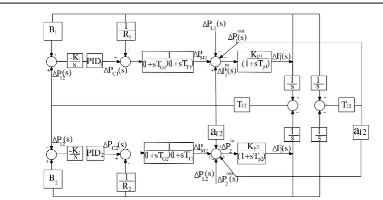
The frequency control model of the two area system but with the additional PID controller is shown in Fig.2. Suppose there is a change in load (∆PLi) in any bus in the system, the frequencies at buses in the

[image:6.595.115.501.68.269.2]

Fig. 2. Propose control block diagram of two-area interconnected system 4. RESULTS AND DISCUSSIONS

4.1. Sub Frequency deviation response in dynamic network model

In this paper, the proposed approach is applied on a 230 kV power system of Fig. 3. The system consists of three thermal generating units, the connected branches that have the same impedances, and the loads that are placed on buses 2, 3, 4 and 5. The frequency deviation response is illustrated with a sudden load increase of 10% (P=0.1 p.u) on bus 3 at t = 0.2s. For the purpose of analysis, performance of the dynamic system model and static model under various scenarios are compared. The system data are given in the Table 1,2,3 and the Induction motors data are η (efficiency) =80%; pf (power factor)= 0.85 lag; Pout = 50HP; and inertia constant HIMi=6. It is assumed that static loads connected to the four buses (bus 2, bus 3, bus 4 and bus

[image:6.595.143.520.382.763.2]

5) have equal power magnitude as induction motors at each respective bus.

Fig. 3. Test system diagram Table 1. Generator data

No.Gen Type H R X’d TG TT DG

1 Steam 9 0.03 1.3125 0.2 0.3 0.1

2 Steam 9 0.03 1.3125 0.2 0.3 0.1

3 Steam 9 0.03 1.3125 0.2 0.3 0.1

Table 2. PID controller data No. PID KP KI KD

1 15 10 7 2 20 15 10

) P 1 R 1 B ) 1 12 p2 1 T + F ( K P 1 G2 1 1+sT 1 (s) 1 P out

a

p2 (s) 2 -s T2 12 ( s s ) (s) (1+sT L2 -K 1+sT + B T K (s) _ + 2 ( p1 +

a

P (s) _ 12 ( L1 P _ + + _ in C2 PID _ P in PID 1 s 2 out 2(s) -K P (s) 2 1 1 s -(s) R C1(s) 12(s) 1 + P 12(s) P _ ) G1 1+sT M1 + + P 2 P + ) 1 M2 + 1 s (1+sT 12 p1 2 1

+ P F

[image:7.595.213.396.94.163.2]

Table 3. Bus data

Bus Vi(pu) i(pu) DL

1 1.017 -1.02

2 1.0566 -2 0.6 3 0.996 -4 0.6 4 1.013 -3.7 0.6 5 1.0566 -2.2717 0.6

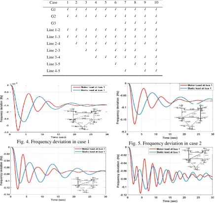
The test network is modeled in the MATLAB/Simulink environment. Several scenarios of connections among generator buses, load buses and power branches listed in Table 4 are considered. The loads are modelled as frequency dependent loads. The responses of the frequency deviations at bus 1 (generator 1) are chosen as a reference bus for comparison between motor loads and static loads under various scenarios as shown in Fig.4 to Fig.13.

Table 4. Cases of changing connected networks

Case 1 2 3 4 5 6 7 8 9 10

G1 √ √ √ √ √ √ √ √ √ √

G2 √ √ √ √ √ √ √ √ √ √

G3 √ √ √ √

Line 1-2 √ √ √ √ √ √ √ √ √ √

Line 1-3 √ √ √ √ √ √ √ √ √ √

Line 2-4 √ √ √ √ √ √ √ √ √

Line 2-3 √ √ √ √ √ √

Line 3-4 √ √ √ √ √ √ √

Line 3-5 √ √ √ √

Line 4-5 √ √ √

[image:7.595.212.397.96.163.2]

Fig. 4. Frequency deviation in case 1 _{Fig. 5. Frequency deviation in case 2}

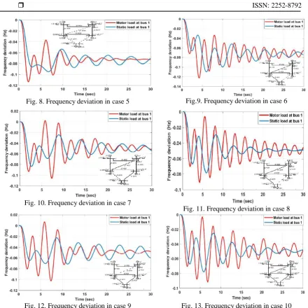
[image:7.595.96.533.256.667.2]

Fig. 8. Frequency deviation in case 5 Fig.9. Frequency deviation in case 6

Fig. 10. Frequency deviation in case 7

Fig. 11. Frequency deviation in case 8

Fig. 12. Frequency deviation in case 9 Fig. 13. Frequency deviation in case 10

Increasing the load by 10% at bus 3, in the case 1 there is small drop in frequency deviation at bus 1 and steady state response time is almost 27 seconds in both static loads and motor loads. However, the frequency deviation at bus 1 increases graduatelly for cases 2 to 10. When adding line 2-4 to network model in the case 2, there is a significant change of frequency at bus 1 and it takes more than 30 seconds to reach the steady state. In the case 3, the oscillation of frequency at bus 1 reduces compared to the case 2 due to there are one more line 2-3 connected to network. In addition, the frequency osscillation and time response are higher for cases 4 to 10. These changes are related to addition of more loads and lines at buses in the network. In general, more incremental oscillations of the frequency deviation response observed at buses with motor loads than the static loads.

4.2. Influence of motor load to the proposed load frequency control response

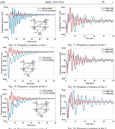
[image:8.595.93.534.55.496.2]

Fig. 14. Frequency response at bus 1 Fig. 17. Frequency response at bus 1

Fig. 15. Frequency response at bus 2 Fig. 18. Frequency response at bus 2

Fig. 16. Frequency response at bus 5 Fig. 19. Frequency response at bus 5 The analysis of Figs.17-19 show that the speed of frequency control response of motor loads is faster than the frequency control response of static loads. This is due to among the motor loads and generators transfer kinertic energy together, they support together and help for frequency responses reaching the steady state quickly.

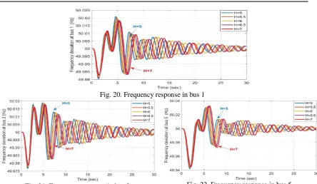
Finally, the different load inertia constants HIMi =(5; 5.5; 6; 6.5; 7) at bus 3 (increase 10% load) are

implemented in the proposed PID control system to gain frequency responses at respective buses in the network. The simulated results are shown in Figs.20-22. The tentative analysis of the obtained results suggest that value of inertia HIMi of the motor has a direct effect on the initial slope and the time of the peak response

[image:9.595.92.532.54.546.2]

Fig. 20. Frequency response in bus 1

Fig. 21. Frequency response in bus 2 Fig. 22. Frequency response in bus 5 5. CONCLUSION

The model of a dynamic network for study into the effect of a small change in load on deviation of local frequencies of the network is presented. The network is composed of generators, load buses and branches between the buses. The proposed dynamic model of the network for analyzing the frequency deviation response is implemented within MATLAB-Simulink environment to compare the effect of static loads and induction motor loads. The proposed dynamic network model can be developed in an interconnected network with multi generator buses, load buses and connected branches. This paper also demonstrates the reliable operation of the PID controller for frequency response and the influence of an induction motor through inertia constants on the characteristics of the proposed load frequency controller. The drawbacks of these PID controllers are fixed control gains while the system changes continuously in time. Also in the frequency stability study, the effects of load dynamics and especially induction motor loads on frequency recovery phenomena need to be considered more seriously.

REFERENCES

[1] N. Lu, D. P. Chassin, and S. E. Widergren, “Modeling uncertainties in aggregated thermostatically controlled loads using a state queueing model,” IEEE Trans. Power Syst., vol. 20, no. 2, pp. 725–733, May 2005.

[2] N. Ruiz, I. Cobelo, and J. Oyarzabal, “A direct load control model for virtual power plant management,” IEEE Trans. Power Syst.,vol.24, no. 2, pp. 959–966, May 2009

[3] H. Omara and F. Bouffard, “A methodology to study the impact of an increasingly nonconventional load mix on primary frequency control,” in Proc. IEEE PES General Meeting, Jul. 2009.

[4] X. Quangghu, C. Chen, S. Qu, The influence of induction motor inerita constant on small-signal stability, Electric Power System Reseach 74 (2005) 192-202.

[5] B.M Weedy, B.J.Cory, N.Jenkins, J.B. Ekanayake, G.Strbac, Electric power system, 3th ed.UK, Wiley, 2012.

[6] L.L.Grigsby, Power system stability and control, 2nd ed. New York, Taylor  Francis Group, 2007.

[7] J. Machowski, J. Bialek, and J. Bumby, Power System Dynamics: Stability and Control, 2nd ed. New York: Wiley, 2008.

[8] D.P. Kothari, Modern power System Analysis, 3th ed. Tata McGraw – Hill, 2009.

[9] P. Patnaik, “Load Frequency in a Single Area Power System”, Barchelor’s thesis, Department of electrical Engineering, National Institude of Technology, Rourkela-769008, May 2013.

[10]A. Usman, B P Divakar, “Simulation Study of Load Frequency Control of Single and Two Area Systems”, in Proc.

IEEE Global Hamanitarian Technology Conference, 2012.

[11]Q. Shi, H. Cui, F Li, Y Liu, W Ju, Y. Sun, “ A Hybrid Dynamic Demand Control Strategy for Power System Frequency Regulation”, CSEE Journal of Power and Energy System, Vol.3, No.2, June 2017.

[12]A. R. B. Azinan, “ Simulation of Dynamic Load Effect on Power System Frequency”, Master’s thesis of Electrical

Engineering with Honors, University Tun Hussein Malaysia, February 2013.

[13]C. Zhao, U. Topcu, and S. H. Low, “Swing dynamics as primal-dual algorithm for optimal load control,” in Proc.

[image:10.595.91.536.69.327.2]

[14]C.E. Fosha, O. I. Elgerd, “The Megawatt-Frequency Control Problem: A New Approach Via Optimal Control Theory”, IEEE Transactions on Power Apparatus and Systems, Vol. Pas-89, No.4, April 1970.

[15]C. Zhao, U. Topcu, N. Li, S. Low, “Design and Stability of Load-Side Primary Frequency Control in Power Systems”,

IEEE Transactions on Automatic Control, Vol.59, NO.5, May 2014.

[16]G. Iovan, I. Mircea, “The Load Frequency Control Simulation in the Interconnected Electrical Power System”,

978-1-4673-1810-5/12/$31.00, 2012 IEEE.

[17]B. Mohanty, S. Panda, P.K. Hota, “Controller Parameters Tuning of Differential Evolution Algorithm and its Application to Load Frequency control of Multi-Source Power System”, Journal homepage: www.elsevier.com/lpcate/ijepes.

[18]I. R. Navarro, “ Dynamic Load Models for Power Systems”, Licentiate thesis, Department of industrila Electrical Engineering and Automation, Lund University, Sweden, 2002.

[19]L.T.M.Trang, H. Nouri, “ Modeling Dynamic Frequency Control with Power Reserve Limitations”, 53rd International Universities Power Engineering Conference (UPEC 2018), 4th – 7th September 2018, 978-1-5386-2910-9/18/$31.00 ©2018 IEEE.

BIOGRAPHIES OF AUTHORS

Le Thi Minh Trang Graduated bacherlor and master in electrical engineering faculty, Hanoi University of Science and Techinology, Vietnam. Now doing Ph.D in Instrumentations and Control department in Czech Technichcal University in Prague, Czech Republic. Main fields are simulation, analysis stability of power system, Fault Locations and Smart Grids.

Hassan Nouri