A stock flow fund ecological macroeconomic model

(1)

A stock-

ﬂ

ow-fund ecological macroeconomic model

Yannis Dafermos

a,

⁎

_{, Maria Nikolaidi}

b

_{, Giorgos Galanis}

c a

Department of Accounting, Economics and Finance, University of the West of England, Bristol, UK b

Department of International Business and Economics, University of Greenwich, London, UK

c_{Institute of Management Studies, Goldsmiths, University of London; New Economics Foundation, London, UK}

a b s t r a c t

a r t i c l e i n f o

Article history: Received 31 January 2016

Received in revised form 22 May 2016 Accepted 12 August 2016

Available online xxxx

This paper develops a stock-flow-fund ecological macroeconomic model that combines the stock-flow consistent approach of Godley and Lavoie with theflow-fund model of Georgescu-Roegen. The model has the following key features. First, monetary and physical stocks andflows are explicitly formalised taking into account the account-ing principles and the laws of thermodynamics. Second, Georgescu-Roegen's distinction between stock-flow and fund-service resources is adopted. Third, output is demand-determined but supply constraints might arise either due to environmental damages or due to the exhaustion of natural resources. Fourth, climate change influences directly the components of aggregate demand. Fifth, finance affects macroeconomic activity and the materialisation of investment plans that determine ecological efficiency. The model is calibrated using global data. Simulations are conducted to investigate the trajectories of key environmental, macroeconomic and finan-cial variables under (i) different assumptions about the sensitivity of economic activity to the leverage ratio of firms and (ii) different types of greenfinance policies.

Ecological macroeconomics Stock-ﬂow consistent modelling Laws of thermodynamics Climate change Finance

1. Introduction

Ecological macroeconomics is an emerging interdisciplinaryfield that examines the macroeconomy as part of the ecosystem, taking ex-plicitly into account the biophysical limits of afinite planet (Jackson, 2009; Rezai et al., 2013; Rezai and Stagl, 2016). It largely draws on the synthesis of ecological economics and post-Keynesian macroeconomics which has been identified as a fruitful avenue for the combined exami-nation of economic and ecological issues (Mearman, 2009; Kronenberg, 2010; Fontana and Sawyer, 2013, 2016).

Recent research has contributed to the development of the building blocks of ecological macroeconomics.Victor and Rosenbluth (2007),

Victor (2012)andBarker et al. (2012) have presented simulation econometric models with Keynesian features that incorporate various environmental issues.Jackson (2009),Fontana and Sawyer (2013),

Rezai et al. (2013)andTaylor et al. (2016)have put forward theoretical frameworks that combine ecological with Keynesian (or post-Keynesian) insights.Berg et al. (2015),Jackson and Victor (2015),

Naqvi (2015)andFontana and Sawyer (2016)have examined environ-mental aspects within stock-ﬂow consistent or monetary circuit models that include aﬁnancial sector.

However, there is still a lack of an integrated ecological macroeco-nomic model that combines physical variables with monetary variables

in a consistent way. This paper develops such a model by combining the stock-flow consistent (SFC) approach ofGodley and Lavoie (2007)with theflow-fund model ofGeorgescu-Roegen (1971, ch. 9; 1979, 1984). Our stock-flow-fund model has the following key features. First, mone-tary and physical stocks andflows are explicitly formalised taking into account the accounting principles and the laws of thermodynamics. Second, Georgescu-Roegen's distinction between stock-flow resources and fund-service resources is adopted. Third, output is demand-determined but supply constraints might arise either due to environ-mental damages or due to the exhaustion of natural resources. Fourth, climate change influences directly the components of aggregate de-mand. Fifth, finance affects macroeconomic activity and the materialisation of investment plans that determine ecological efficiency. The model is calibrated using global data. Simulations are conducted to illustrate the channels through which the ecosystem, thefinancial sys-tem and the macroeconomy interact. Particular attention is paid to the non-neutral role of finance in the ecosystem-macroeconomy interactions.

The paper is organised as follows.Section 2describes brieﬂy the foundations of the model.Section 3analyses the structure of the model.Section 4presents our simulation analysis.Section 5summarises and concludes.

2. Foundations of the model

The key innovation of the post-Keynesian SFC approach developed byGodley and Lavoie (2007)is the explicit integration of accounting ⁎ Corresponding author at: University of the West of England, Frenchay Campus,

Coldharbour Lane, Bristol BS16 1QY, UK.

E-mail address:[email protected](Y. Dafermos).

http://dx.doi.org/10.1016/j.ecolecon.2016.08.013

Contents lists available atScienceDirect

Ecological Economics

(2)

into dynamic macro modelling. This integration permits the detailed ex-ploration of the links between the real and theﬁnancial spheres of the macroeconomy. However, a prominent drawback of the SFC models is that they ignore the transformation of matter and energy that takes place due to economic processes and the environmental problems caused by this transformation. This feature comes in stark contrast with the fundamental propositions of ecological economists according to which the macroeconomy is part of the ecosystem and economic ac-tivity unavoidably respects the laws of thermodynamics (seeDaly and Farley, 2011).

Theflow-fund model ofGeorgescu-Roegen (1971, ch. 9; 1979; 1984)encapsulates the fundamental propositions of ecological eco-nomics. His model relies on a multi-process matrix that depicts the physical inflows and outflows that take place during the various eco-nomic processes, drawing explicitly on the First and the Second Law of Thermodynamics. His model also makes a crucial distinction between the stock-flow resources and the fund-service resources (see also

Mayumi, 2001; Kurz and Salvadori, 2003; Daly and Farley, 2011). The stock-ﬂow resources (non-renewable energy and material resources) are transformed into what they produce (including by-products), can theoretically be used at any rate desired and can be stockpiled for future use. The fund-service resources (labour, capital and Ricardian land) are not embodied in the output produced, can be used only at speciﬁc rates and cannot be stockpiled for future use. Crucially, these types of re-sources are not substitutable: they are both necessary for the produc-tion process.

Our stock-flow-fund ecological macroeconomic model integrates the post-Keynesian SFC approach with Georgescu-Roegen'sfl ow-fund model. The model that we develop relies on four matrices: 1) the physicalflow matrix; 2) the physical stock-flow matrix; 3) the transactionsflow matrix; 4) the balance sheet matrix. The first matrix is a simplification of the matrix that Georgescu-Roegen's used in hisflow-fund model. The second matrix captures the dynamic interaction between physical stocks andflows and is a natural extension of the physicalflow matrix. The third matrix and the fourth matrix describe the changes in the stocks andflows of the macroeconomic and thefinancial system, following the tradi-tional formulations in the SFC literature.

In line with the post-Keynesian tradition, output in the model is de-termined by aggregate demand. However, supply-side constraints might arise primarily due to environmental problems. This is formalised by using a Leontief-type production function that speci_fies the supply-determined output drawing on Georgescu-Roegen's distinction be-tween stock-flow and fund-service resources. It is assumed that envi-ronmental problems affect in a different way each type of resources. Depletion problems affect the stock-flow resources (i.e. non-renewable energy and material resources can be exhausted) while deg-radation problems, related to climate change and the accumulation of hazardous waste, damage the fund-service resources (by destroying them directly or by reducing their productivity). Climate change and its damages are modelled using standard specifications from the inte-grated assessment modelling literature (seeNordhaus and Sztorc, 2013). However, a key departure from this literature is that global warming damages do not affect in our model an output determined via a neoclassical production function. Instead, they influence the fund-service resources of our Leontief-type production function and the components of aggregate demand.

3. Structure of the model

The model portrays the global macroeconomy without a govern-ment sector. There is one type of material good that can be used for du-rable consumption and (conventional and green) investment purposes. Firms produce this good by using: (i) matter which has to be extracted from the ground (non-metallic minerals and metal ores); (ii) matter that has been recycled using demolished/discarded socio-economic

stock1_{; and (iii) energy that comes either from non-renewable sources} (e.g. oil, gas and coal) or renewable sources (e.g. sun, wind).2_The by-products of the production process are CO2emissions, waste and

dissi-pated energy.3

Production can be made by using either green capital or convention-al capitconvention-al. Compared to conventionconvention-al capitconvention-al, green capitconvention-al is characterised by lower energy intensity, lower material intensity and higher recycling rate. Moreover, green capital produces energy using renewable sources while conventional capital produces energy using non-renewable sources. Hence, the use of green capital is conducive to a low-carbon economy.

Firms invest in conventional and green capital by using retained profits and loans. Banks impose credit rationing onfirm loans, playing thereby a crucial role in the determination of output and the accumula-tion of green capital. Households provide their labour services tofirms. They buy durable consumption goods and accumulate wealth in the form of deposits. They do not take out loans. Commercial banks distrib-ute all their profits to households. To avoid complications related to in-flation, it is assumed that the price of consumption and investment goods is constant and equal to unity. Using US dollar ($) as a reference currency, this means that each good values 1 US$.

3.1. Ecosystem

Table 1depicts the physicalflow matrix of our model. This matrix captures the First and the Second Law of Thermodynamics. The First Law of Thermodynamics implies that energy and matter cannot be cre-ated or destroyed when they are transformed during the economic pro-cesses. This is re_flected in the material and energy balance. The_first column inTable 1depicts the material balance in Gigatonnes (Gt).4 Ac-cording to this balance, the total inputs of matter into the socio-economic system over a year (extracted matter, the carbon mass of non-renewable energy and the oxygen included in CO2emissions)

should be equal to the total outputs of matter over the same year (in-dustrial CO2emissions and waste) plus the change in socio-economic

stock. The second column inTable 1depicts the energy balance in Exajoules (EJ). According to this balance, the total inputs of energy into the socio-economic system over a year should be equal to the total outputs of energy over the same year. Symbols with a plus sign de-note inputs into the socio-economic system. Symbols with a minus sign denote outputs or changes in socio-economic stock. The Second Law of Thermodynamics is captured by the fact that the economic processes transform low-entropy energy (e.g. fossil fuels) into high-entropy dissi-pated energy (e.g. thermal energy).

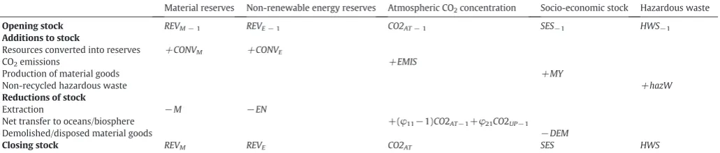
Table 2displays the physical stock-ﬂow matrix of our model.5This matrix presents the dynamic change in those physical stocks that are considered more important for human activities. These are the material and non-renewable energy reserves, the atmospheric CO2

concentra-tion, the socio-economic stock and the stock of hazardous waste. The ﬁrst row of the matrix shows the stocks of the previous year. The last row presents the stocks at the end of the current year after the additions to stocks and the reductions of stocks have taken place. Additions are denoted by a plus sign. Reductions are denoted by a minus sign.

The reserves of matter and non-renewable energy are those volumes expected to be produced economically using the existing technology. The reserves stem from the resources which are the volumes presenting

1 _{The socio-economic stock includes capital goods and durable consumption goods.} 2

For brevity, the energy produced from (non-)renewable sources is henceforth referred to as (non-)renewable energy in the paper.

3

For simplicity, the model does not incorporate energy and matter from biomass. How-ever, theﬁgure used for the share of renewable energy in our calibrations includes bioenergy to facilitate comparison with other studies.

4 _{For the use of the material balance in material}_ﬂ_{ow accounting see}_{Fischer-Kowalski} et al. (2011).

5

(3)

technical difﬁculties, are costly to extract or have not yet been discov-ered. When resources are converted into reserves, it means that people have a higher stock of matter and energy to rely on for economic pro-cesses. Note that although this conversion is important for human activ-ities, it does not represent a physical transformation.

Tables 1 and 2imply that in our model the laws of thermodynamics are important for three reasons. First, the First Law of Thermodynamics allows us to incorporate explicitly the harmful by-products of energy and matter transformation (CO2emissions and hazardous material

waste). As will be explained below, these by-products cause the degra-dation of ecosystem services with feedback effects on the economy. Sec-ond, the Second Law of Thermodynamics implies that in the very long run the economic processes cannot rely on the energy produced from fossil fuels. Since the fossil fuel resources areﬁnite and the economic processes transform the low-entropy energy embodied in these re-sources into high-entropy energy, sustainability requires the reliance of economic processes on renewable energy sources (even if there was no climate change). Third, by combining the laws of thermodynam-ics with Georgesu-Roegen's analysis of material degradation, it turns out that recycling might not be sufﬁcient to ensure the availability of the material resources that are necessary for the economic processes. Hence, the depletion of matter needs to be checked separately.

We proceed to describe the equations of the model that refer to the ecosystem.

3.1.1. Matter, recycling and waste

MY¼μY ð1Þ

M_¼MY₋REC _ð2_Þ

REC¼ρDEM ð3Þ

DEM¼μ δðK₋1þξDC−1Þ ð4Þ

SES¼SES₋1þMY−DEM ð5Þ

W¼MþCENþO2−EMISIN−ΔSES ð6Þ

CEN¼EMISIN

car ð7Þ

O2¼EMISIN−CEN ð8Þ

HWS¼HWS₋1þhazW ð9Þ

hazrario¼HWS

SURF ð10Þ

REVM¼REVM−1þCONM−M ð11Þ

CONM¼conMRESM−1 ð12Þ

RESM¼RESM−1−CONM ð13Þ

depM¼

M

REVM−1 ð

14Þ

The goods produced every year (Y) embody a speciﬁc amount of matter,MY(Eq.(1)). Material intensity (μ) is deﬁned as the matter in-cluded in each output produced. Not all of the matter embodied in the produced output needs to be extracted from the ground (M). As shown in Eqs.(2) and (3), a part ofMYcomes from the amount of demolished/discarded socio-economic stock that is recycled (REC);ρ denotes the recycling rate. The demolished/discarded socio-economic stock (DEM) is equal to the material content of the depreciated capital goods and the end-of-life durable consumption goods (Eq.(4));δis the depreciation rate of capital goods (K) andξis the proportion of du-rable consumption goods (DC) discarded every year. Eq.(5)shows that socio-economic stock (SES) increases as a result of the production of new goods and decreases due to the demolition/discard of old material goods.

Eq.(6)reﬂects the material balance depicted inTable 1. The waste (W) generated during the production process is used as a residual. Re-garding non-renewable energy, only its carbon mass,CEN, has been in-cluded as input in the material balance. As shown in Eq.(7), this mass is estimated from the industrial emissions (EMISIN) by using the conver-sion rate of Gt of carbon into Gt of CO2(car). Carbon exits the

socio-economic system in the form of CO2emissions. Oxygen (O2) is

intro-duced as an input in the material balance because it is necessary in the fossil fuel combustion process. Eq.(8)gives the mass of the oxygen that is part of the CO2emissions. Note that by combining Eqs.(2), (5), (6) and (8)it can be easily shown thatW=DEM−REC.

Table 1

Physicalﬂow matrix.

Material balance Energy balance

Inputs

Extracted matter +M

Renewable energy +ER

Non-renewable energy +CEN +EN

Oxygen +O2

Outputs

Industrial CO2emissions −EMISIN

Waste −W

Dissipated energy −ED

Change in socio-economic stock −ΔSES

Total 0 0

[image:3.595.47.563.624.734.2]

Note: The table refers to annual globalﬂows. Matter is measured in Gt and energy is mea-sured in EJ.

Table 2

Physical stock-ﬂow matrix.

Material reserves Non-renewable energy reserves Atmospheric CO2concentration Socio-economic stock Hazardous waste

Opening stock REVM−1 REVE−1 CO2AT−1 SES−1 HWS−1

Additions to stock

Resources converted into reserves +CONVM +CONVE

CO2emissions +EMIS

Production of material goods +MY

Non-recycled hazardous waste +hazW

Reductions of stock

Extraction −M −EN

Net transfer to oceans/biosphere +(φ11−1)CO2AT−1+φ21CO2UP−1

Demolished/disposed material goods −DEM

Closing stock REVM REVE CO2AT SES HWS

(4)

Only a small proportion (haz) of the waste produced every year is hazardous, i.e. it is harmful to human health or the environment.6_This hazardous waste is added to the accumulated stock of hazardous waste,HWS(Eq.(9)). Eq.(10)deﬁnes the hazardous waste accumula-tion ratio which expresses the accumulated stock of hazardous waste in Gt per million km2_{of earth surface (}_SURF_).

The material stock-ﬂow dynamics are presented in Eqs.(11)–(14). Eq.(11)shows that the material reserves (REVM) decline when matter is extracted and increase when resources are converted into reserves. The annual conversion (CONM) is given by Eq.(12). An exogenous con-version rate,conM, has been assumed. Eq.(13)describes the change in material resources (RESM). To capture the scarcity of matter we deﬁne the matter depletion ratio (depM), which is the ratio of matter that is ex-tracted every year relative to the remaining material reserves (Eq.(14)). The higher this ratio the greater the matter depletion problems.

3.1.2. Energy

E¼εY ð15Þ

ER_¼_θE _ð16_Þ

EN¼E−ER ð17Þ

ED¼ENþER ð18Þ

REVE¼REVE−1þCONE−EN ð19Þ

CONE¼conERESE−1 ð20Þ

RESE¼RESE−1−CONE ð21Þ

depE¼

EN

REVE−1 ð

22Þ

The energy required for production (E) is a function of output (Eq.(15)). When energy intensity (ε) declines, the energy required per unit of output becomes lower. As shown in Eqs.(16) and (17), ener-gy is generated either from renewable (ER) or non-renewable sources (EN). The share of renewable energy in total energy is denoted byθ. The dissipated energy (ED) is determined based on the energy balance (Eq.(18)).

Eqs.(19)–(22)represent the stock-ﬂow dynamics of the energy pro-duced from non-renewables. Eq.(19)shows the change in the non-renewable energy reserves (REVE).CONEdenotes the amount of re-sources converted into reserves every year. This amount is determined by Eq.(20), whereconEis the conversion rate. The resources of non-renewable energy (RESE) change every year according to Eq.(21). The energy depletion ratio, which captures scarcity problems, shows the ex-tracted energy relative to the remaining reserves (Eq.(22)).

3.1.3. Emissions and climate change

EMISIN¼ωEN ð23Þ

EMISL¼EMISL−1ð1−lrÞ ð24Þ

EMIS¼EMISINþEMISL ð25Þ

CO2AT¼EMISþϕ11CO2AT−1þϕ21CO2UP−1 ð26Þ

CO2UP¼ϕ12CO2AT−1þϕ22CO2UP−1þϕ32CO2LO−1 ð27Þ

CO2LO¼ϕ23CO2UP−1þϕ33CO2LO−1 ð28Þ

F¼F2CO2log2 CO2AT

CO2AT−PREþ

FEX ð29Þ

FEX¼FEX−1þfex ð30Þ

TAT¼TAT−1þt1 F− F2CO2

S TAT−1−t2ðTAT−1−TLO−1Þ

ð31Þ

TLO¼TLO−1þt3ðTAT−1−TLO−1Þ ð32Þ

Our formalisation of emissions and climate change follows closely the traditional integrated assessment models (see Nordhaus and Sztorc, 2013). Every year industrial CO2emissions (EMISIN) are

generat-ed due to the use of the non-renewable energy sources (Eq.(23)). CO2

intensity (_ω) is de_ﬁned as the industrial emissions produced per unit of non-renewable energy. Every year land-use CO2emissions (EMISL)

are also generated because of changes in the use of land (Eq.(24)). These emissions are assumed to decline exogenously at a ratelr. Eq.(25)gives the total emissions (EMIS).

The atmospheric CO2concentration (CO2AT) is driven by these emis-sions and the carbon cycle. The carbon cycle, represented by Eqs.(26)–(28), shows that every year there is exchange of carbon be-tween the atmosphere and the upper ocean/biosphere and bebe-tween the upper ocean/biosphere and the lower ocean;CO2UPis the upper ocean/biosphere CO2concentration andCO2LOis the lower ocean CO2

concentration. The higher the net transfers of carbon from the atmo-sphere into the other two reservoirs the lower the atmospheric CO2

con-centration. The accumulation of atmospheric CO2and other greenhouse

gases increases radiative forcing,F(Eq.(29)), placing upward pressures on the atmospheric temperature,TAT(Eq.(31)).F2×CO2is the increase in

radiative forcing (since the pre-industrial period) due to doubling of CO2concentration from pre-industrial levels (CO2AT–PRE). For simplicity, the radiative forcing due to non-CO2greenhouse gas emissions (FEX) is

determined exogenously (Eq.(30)). Eq.(32)shows the change in the temperature of the lower ocean (TLO).

3.1.4. Ecological efﬁciency and technology

ω¼ω−1ð1þg_ωÞ ð33Þ

g_ω¼g_ω₋1ð1−ζ1Þ ð34Þ

μ¼κ−1μGþð1−κ−1ÞμC ð35Þ

μG¼μG−1 1þgμG

ð36Þ

g_μG¼gμG−1ð1−ζ2Þ ð37Þ

ρ¼κ−1ρGþð1−κ−1ÞρC ð38Þ

ρG¼ρG−1 1þgρG

ð39Þ

g_ρG¼gρG−1ð1−ζ3Þ ð40Þ

ε¼κ−1εGþð1−κ−1ÞεC ð41Þ

εG¼εG−1ð1þgεGÞ ð42Þ

g_εG¼gεG−1ð1−ζ4Þ ð43Þ

θ¼ 1þ_π_K 1 G−1=KC−1

ð Þ

−1

ð44Þ 6

(5)

The ecological efﬁciency of production is considered to be higher the lower is the energy, material and CO2intensity and the higher is the

recycling rate. Ecological ef_ﬁciency also increases when the share of re-newable energy in total energy goes up. CO2intensity changes in an

ex-ogenous way. As shown in Eqs.(33) and (34), every year technical progress reduces CO2 intensity with a declining rate (gωb0 and ζ1N0).7Material intensity, energy intensity and recycling rate are not

af-fected only by exogenous technical progress. Since green capital is characterised by lower material and energy intensity and by higher recycling rate, the efficiency related to these indicators increases when the ratio,κ, of green capital (KG) to total capital (K) rises. This is shown in Eqs.(35), (38) and (41)whereμG,ρGandεGdenote, respec-tively, the material intensity, recycling rate and energy intensity of green capital andμC,ρCandεCare the respective indicators for conven-tional capital. Eqs.(36), (37), (39), (40), (42) and (43)reflect the fact that exogenous technical progress improves (with a declining rate) the ecological efficiency of green capital (gμGb0, gρGN0,gεGb0, ζ2N0,ζ3N0 andζ4N0). The ecological efficiency of conventional

cap-ital is assumed to be constant. The share of renewable energy in total en-ergy (θ) is higher the higher is the ratio of green capital stock to conventional capital stock (Eq.(44)).

[image:5.595.309.543.57.301.2]

3.2. Macroeconomy andﬁnancial system

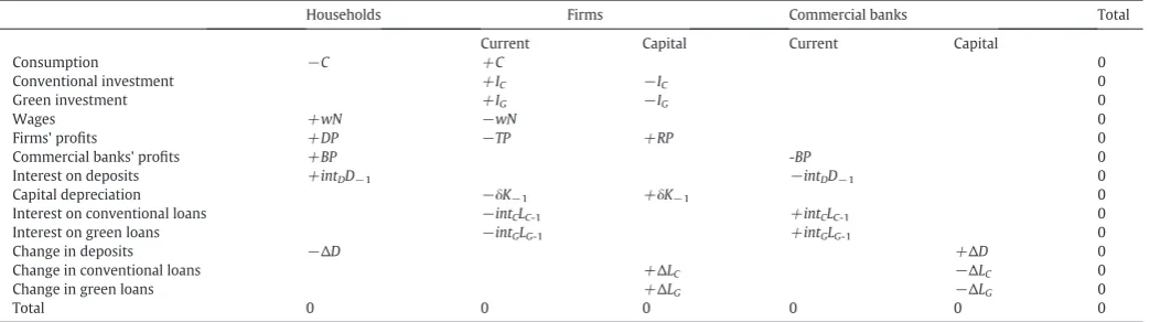
Table 3andTable 4portray the transactionsflow matrix and the bal-ance sheet matrix of our macroeconomy (these types of matrices have been presented in detail byGodley and Lavoie, 2007). The transactions flow matrix shows the transactions that take place between the various sectors of the economy (each row represents a category of transac-tions). For each sector inflows are denoted by a plus sign and outflows are denoted by a minus sign. The upper part of the matrix shows trans-actions related to the revenues and expenditures of the various sectors. The bottom part of the matrix indicates changes infinancial assets and liabilities that arise from transactions. The columns represent the bud-get constraints of the sectors. Forfirms and commercial banks a distinc-tion is made between current and capital accounts. The current accounts register payments made or received. The capital accounts show the changes in assets and liabilities as well as the funds that are used tofinance investment (in the case offirms). At the aggregate level, monetary inflows are equal to monetary outflows.

Table 4shows the assets and the liabilities of the sectors. We use a plus sign for the assets and a minus sign for the liabilities. Households andfirms have non-zero net worth. Commercial banks have a zero net worth due to the assumption that they distribute all their profits. Ac-counting requires that at the aggregate levelfinancial assets are equal tofinancial liabilities. Hence, the net worth of the economy is equal to the real assets which include the capital stock offirms and the durable consumption goods of households.

In the next subsections we present the equations for the macroeconomy and theﬁnancial system.

3.2.1. Output determination and damages

Y_M¼REVM−1þREC

μ ð45Þ

YE¼

REVE−1 1−θ

ð Þε ð46Þ

YK¼vK ð47Þ

YN¼λhLF ð48Þ

Y¼min YM;YE;YK;YN

ð49Þ

Y¼CþI ð50Þ

um¼_YY

M ð

51Þ

ue¼_YY E

ð52Þ

u¼_YY

K ð

53Þ

re¼_YY

N ð

54Þ

DT¼1−

1

1þη1TATþη2TAT2þη3TAT6:754

ð55Þ

DTP¼pDT ð56Þ

DTF¼1−

1−DT

1₋DTP ð

57Þ

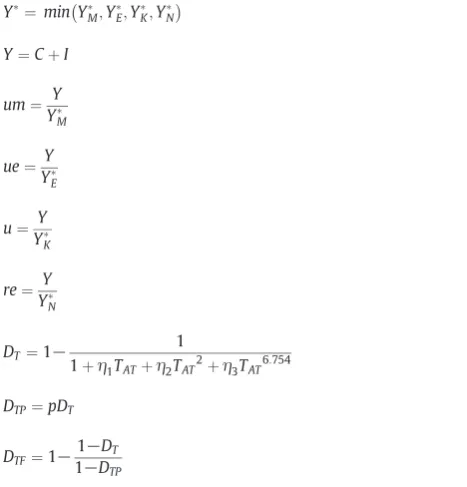
We assume a Leontief-type production function that incorporates Georgescu-Roegen's distinction between stock-flow and fund-service resources. The stock-flow resources are matter and non-renewable en-ergy. The fund-service resources are labour and capital. We define four different types of potential output. The matter-determined potential output (YM⁎) is defined in Eq.(45)and is higher the higher are the mate-rial reserves, the higher is the recycled matter and the lower is the ma-terial intensity. The energy-determined potential output (YE⁎) is defined in Eq.(46)and is higher the higher are the non-renewable energy re-serves, the lower is the energy intensity and the higher is the share of renewable energy in total energy. The capital-determined potential out-put (YK⁎) is defined in Eq.(47)and is higher the higher is the capital stock and the productivity of capital (v). Lastly, the labour-determined potential output (YN⁎) is defined in Eq.(48)and is higher the higher is the labour force (LF), the hourly labour productivity (λ) and the annual working hours per employee (h). The overall potential output (Y⁎) is the minimum of all these potential outputs (Eq.(49)).

In line with the post-Keynesian tradition, actual output (Y) is demand-determined (Eq.(50)): it is equal to consumption demand (C) plus investment demand (I). However, as shown in Eqs.(62)–(67)

below, demand is not independent of supply. When actual output ap-proaches potential output, demand tends to decline as a result of supply-side constraints. We define four ratios which capture the extent to which potential output is utilised (Eqs.(51)–(54)). Thefirst two ra-tios are the matter utilisation rate (um) and the energy utilisation rate (ue), which refer to the use of stock-flow resources. When these ratios increase, the output produced approaches the potential output deter-mined by the material and energy reserves. The last two ratios are the utilisation rate (u) and the rate of employment (re) which refer to the use of fund-service resources. A rise in these ratios reflects a higher scar-city of capital and labour.

Global warming causes damages to the fund-service resources (cap-ital and labour), reducing thereby the potential output determined by them. There are two types of damages: the damages that affect directly the funds (capital stock and labour force) and the damages that affect the productivities of the funds (capital productivity and labour produc-tivity). Capital stock is affected because climate change can destroy in-frastructure by causing storms or inundations, or it can trigger the abandonment of capital in coastal areas by causing a rise in the sea level (seeDietz and Stern, 2015; Naqvi, 2015; Taylor et al., 2016). Labour force can be reduced since climate change can adversely affect morbid-ity, mortalmorbid-ity, air quality and the vector and proliferation of infectious 7

(6)

diseases. It can also lead to storms andﬂoods that injure and kill people (Toll, 2002). All these phenomena might reduce the population or the proportion of the population that can participate in the labour force. Capital productivity can be driven down since climate change might create a hostile environment that can reduce the ability ofﬁrms to use capital effectively (Stern, 2013; Dietz and Stern, 2015). Finally, by affect-ing the health of the workers, the rise in temperature might decrease their ability to perform work tasks, reducing labour productivity (Kjellstrom et al., 2009; Dell et al., 2014; Taylor et al., 2016).

Aggregate demand is affected by these damages in two ways. First, the catastrophes caused by climate change might increase the fears of entrepreneurs that their capital will be destroyed or that it will have very low returns. This reduces their desired investment.8Moreover, ob-serving the natural disasters and the health problems, households might be induced to save more for precautionary reasons. This can lead to less consumption. Measures that restrict consumption directly might also be adopted. Second, since global warming damages tends to reduceYK⁎andYN⁎, they place upward pressures onuandre. As men-tioned above, this rise in the scarcity of capital and labour can reduce demand.

Importantly, societies do not react passively to the climate change-related effects on fund-service resources. They take adaptation mea-sures that limit global warming damages. Followingde Bruin et al. (2009), we thereby make a distinction between gross damages and net damages. Gross damages are the initial damages caused by climate change if there were no adaptation measures and net damages are the damages that remain after the implementation of adaptation measures.9

Eq.(55)is the damage function, which shows how atmospheric temperature and damages are linked.DTis the proportional gross dam-age which lies between 0 (no damdam-age) and 1 (complete catastrophe). The form of Eq.(55)has been suggested byWeitzman (2012)who ar-gues that the quadratic forms of damage functions used in the tradition-al literature of integrated assessment models do not adequately capture high-temperature damages. This issue is tackled by inserting the term η3TAT6:754whereη3and the corresponding exponent have been selected

such thatDT= 0.5 whenTAT=6 °C.

In most integrated assessments modelsDT affects directly the supply-determined output. On the contrary, as mentioned above, in our modelDTaffects the potential output and the aggregate demand. Hence, the variableDTenters into both (i) the determination of funds and their productivities (see Eqs.(84), (85), (88) and (96)) and (ii) the consumption and investment demand (see Eqs.(62) and (93)). It

is also necessary to partition the gross damage between the fund (DTF) and its productivity (DTP), so as to warrant that whenDT=x% the capital-determined potential output and the labour-determined poten-tial output would be reduced byx% if there were no adaptation mea-sures. This is done by Eqs.(56) and (57).10

The impact of adaptation is captured by the parametersadp,adkand adLFthat represent the proportion of the gross damage (of productivity, capital stock and labour force respectively) which is eliminated due to adaptation measures. We have that 0≤adP,adK,adLF≤1. This means that, for example, the proportional net damage to productivity is given by (1−adP)DTP. We assume that adaptation does not affect investment and consumption demand:ﬁrms and households make decisions based on gross damages.

3.2.2. Firms

TP¼Y−wN−intCLC−1−intGLG−1−δK−1 ð58Þ

RP¼sFTP−1 ð59Þ

DP¼TP−RP ð60Þ

r¼RP=K ð61Þ

ID

¼½ðα0þα1r−1þα2u−1−α3g_ε₋1ÞK−1þδK−1ð1−DT−1Þ ð62Þ

α0¼α00−γ1ðum−1−umTÞ−γ2ðue−1−ueTÞ−γ3ðu−1−uTÞ−γ4ðre−1−reTÞ ð63Þ

γ1¼γ10 iff um−1≥umT; otherwise γ1¼0 ð64Þ

γ2¼γ20 iff ue−1≥ueT; otherwise γ2¼0 ð65Þ

γ3¼γ30 iff u−1≥uT; otherwise γ3¼0 ð66Þ

γ4¼γ40 iff re−1≥reT; otherwise γ4¼0 ð67Þ

ID G¼βI

D

ð68_Þ

IDC¼I D

−IDG ð69Þ

β¼β0þβ1−β2ðintG−intCÞ þβ3DT−1 ð70Þ

β0¼β0−1 1þgβ0

ð71Þ 8

Taylor et al. (2016)have postulated a negative impact of climate change on invest-ment demand by assuming that greenhouse gas concentration reduces the proﬁt share.

9

We do not include theﬁnancial cost of the adaptation measures in net damages. 10

[image:6.595.34.556.77.223.2]

See alsoMoyer et al. (2014).

Table 3

Transactionsﬂow matrix.

Households Firms Commercial banks Total

Current Capital Current Capital

Consumption −C +C 0

Conventional investment +IC −IC 0

Green investment +IG −IG 0

Wages +wN −wN 0

Firms' proﬁts +DP −TP +RP 0

Commercial banks' proﬁts +BP -BP 0

Interest on deposits +intDD−1 −intDD−1 0

Capital depreciation −δK−1 +δK−1 0

Interest on conventional loans −intCLC-1 +intCLC-1 0

Interest on green loans −intGLG-1 +intGLG-1 0

Change in deposits −ΔD +ΔD 0

Change in conventional loans +ΔLC −ΔLC 0

Change in green loans +ΔLG −ΔLG 0

Total 0 0 0 0 0 0

(7)

g_β0¼gβ0−1ð1−ζ5Þ ð72Þ

NLDG¼I D

G−βRPþrepLG−1−δKG−1 ð73Þ

NLD

C¼IDC−ð1−βÞRPþrepLC−1−δKC−1 ð74Þ

IG¼βRPþðLG−LG−1Þ þδKG−1 ð75Þ

IC¼RPþðLC−LC−1Þ þðLG−LG−1Þ þδK−1−IG ð76Þ

I¼ICþIG ð77Þ

L¼LCþLG ð78Þ

KG¼KG−1þIG−δKG−1 ð79Þ

KC¼KC−1þIC−δKC−1 ð80Þ

K¼KCþKG ð81Þ

κ¼KG=K ð82Þ

lev¼L=K ð83Þ

δ¼δ0þð1−δ0Þð1−adKÞDTF−1 ð84Þ

v¼v₋1ð1þgvÞ½1−ð1−adPÞDTP−1 ð85Þ

g_λ¼σ0þσ1þσ2gY−1 ð86Þ

σ0¼σ0−1ð1−ζ6Þ ð87Þ

λ¼λ−1ð1þgλÞ½1−ð1−adPÞDTP−1 ð88Þ

w¼sWλh ð89Þ

N¼_hY_λ ð90Þ

ur¼1−re ð91Þ

The total profits offirms (TP) are given by Eq.(58);wis the wage rate,Nis the number of employed workers,intCis the interest rate on conventional loans,intGis the interest rate on green loans,LCis the amount of conventional loans,LGis the amount of green loans andδis the depreciation of capital stock (which is assumed to be the same for green capital and conventional capital). Firms' retained profits (RP) are a proportion (sF) of their total profits (Eq.(59)). The distributed profits offirms (DP) are determined as a residual (Eq.(60)). Eq.(61)

gives the rate of retained proﬁts (r).

Firms' investment is formalised as a two-stage process. At afirst stage,firms decide their overall desired investment in both green and conventional capital. At a second stage, they allocate their desired in-vestment between the two types of capital. Eq.(62)captures thefirst

stage. The desired investment (ID_{), adjusted for the damage effect, is} equal to net investment plus the depreciated capital. As in most Kaleckian models, net investment is a positive function of the rate of (retained) profits and the rate of capacity utilisation. We also postulate that investment depends on the growth rate of energy intensity (gε) to capture the rebound effect associated with a lower growth rate of ener-gy intensity. The idea is that a lower enerener-gy intensity reduces the costs of production inducingfirms to invest more. This increases their energy use outweighing partially the beneficial effects of a lower energy intensity.11

Eqs.(62)–(67)show that investment demand is reduced when actu-al output approaches potentiactu-al output (γ10,γ20,γ30,γ40N0). In

particu-lar, when the utilisation of matter passes theumTthreshold and/or the utilisation of energy passes theueTthreshold, investment demand is curbed because the prices of matter and energy rise significantly as a re-sult of scarcity, leading to higher production costs. Additionally, when the rate of capacity utilisation and the rate of employment are higher than the thresholdsuTandreTrespectively, labour and capital shortages could lead to rising wages and prices that, under certain conditions, af-fect negatively investment demand. Labour shortages also makefirms uncertain about their ability to recruit workers, deteriorating business confidence (seeRyoo and Skott, 2008; Lavoie, 2014, ch. 6).

The second stage of the investment process is reflected in Eqs.(68)–(72). At this stagefirms decide about the proportion,β, of green investment (IGD) in the overall desired investment (Eq.(68)). De-sired conventional investment (ICD_{) is determined as a residual} (Eq.(69)). The proportion of green investment depends on three factors (Eq.(70)). Thefirst factor is captured by the termβ0+β1which reflects

exogenous developments, such as the cost of installing and using green capital relative to conventional capital or institutional changes that pro-mote green investment. It is assumed thatβ0increases every year but

with a declining rate (Eqs.(71)_–(72))._β1is constant but can change

due to exogenous institutional or technology shocks. The second factor is the divergence between the interest rate on green loans and the inter-est rate on conventional loans. The interinter-est rate differential captures the borrowing cost of investing in green capital relative to conventional capital.12_{The third factor is captured by the variable}_DT_{which re}_ﬂ_ects the fact that climate change might lead to mitigation measures that pro-mote green investment or may induce entrepreneurs to make invest-ments that are conducive to less environmental damage.

Due to the existence of credit rationing, only a proportion of the new loans that are demanded byfirms are provided by banks.13_Eq.₍₇₃₎ gives the desired new green loans (NLGD_{) and Eq.}₍₇₄₎_{gives the desired} new conventional loans (NLCD_{). The green, conventional and total} invest-ment goods after credit rationing are shown in Eqs.(75)–(77);IGis green investment andICis conventional investment. The total loans of firms (L) are equal to conventional loans plus green loans (Eq.(78)). The change in green and conventional capital stock is equal to gross in-vestment minus the depreciation of capital (Eqs.(79) and (80)). Eq.(81)shows that total capital (K) is equal to conventional capital (KC) plus green capital (KG). The ratio of green capital to total capital is given by Eq.(82). The leverage ratio offirms (lev) is defined in Eq.(83).

Eq.(84) shows the rate of capital depreciation. Interestingly, a higher depreciation due to climate change has two countervailing ef-fects on economic growth. On the one hand, capital-determined poten-tial output is reduced, placing adverse supply-side effects on economic activity (see Eq.(47)). On the other hand, aggregate demand tends to

11

For a description of the rebound effects seeBarker et al. (2009). In our modelfirms' payments on energy are netted out due to the consolidation of thefirm sector. Therefore, a lower energy intensity does not affect the aggregate profitability offirms. However, it is crucial to incorporate the expansionary effect of lower energy intensity into the invest-ment function; otherwise, improveinvest-ments in energy efficiency would have only beneficial effects on energy use.

12

For some empirical evidence about the effects of interest rates on green investment seeEyraud et al. (2013).

13

See alsoDafermos (2012)andNikolaidi (2014).

Table 4

Balance sheet matrix.

Households Firms

Commercial banks Total

Conventional capital +KC +KC

Green capital +KG +KG

Durable consumption goods +DC +DC

Deposits +D -D 0

Conventional loans −LC +LC 0

Green loans −LG +LG 0

Total (net worth) +VH +VF 0 +KC+ KG+ DC

(8)

increase because a higher depreciation leads to higher gross investment (see Eq.(62)).

Eqs.(85)_–(88)refer to capital and labour productivity. As argued above, both productivities are inﬂuenced by climate change. Capital productivity, before damages, is assumed to grow at an exogenous rate,gv. Labour productivity is affected by exogenous technology factors reﬂected in the termσ0+σ1. These factors increase productivity growth

every year but with a declining rate. Also, is line with the Kaldor-Verdoorn law (seeLavoie, 2014, ch. 6), the growth rate of labour pro-ductivity is positively affected by the growth rate of output (gY). Note that, although a lower labour productivity can reduce the unemploy-ment rate for a given level of output, it has adverse effects on the supply side by driving down the labour-determined potential output (see Eq.(48)).

Eq.(89)gives the wage rate. The wage share (sW) is assumed to be exogenous. The number of employees is determined by Eq.(90). The unemployment rate is deﬁned in Eq.(91).

3.2.3. Households

YH¼wNþDPþBPþintDD−1 ð92Þ

C¼ðc1YH−1þc2D−1Þð1−DT−1Þ ð93Þ

D¼D₋1þYH−C ð94Þ

DC¼DC−1þC−ξDC−1 ð95Þ

LF¼L F₋1ð1þgLFÞ½1−ð1−adLFÞDTF−1 ð96Þ

gLF¼lf0þlf1−lf2ur−1−lf3hazratio−1 ð97Þ

lf0¼lf0−1ð1−ζ7Þ ð98Þ

Eq.(92)gives the disposable income of households (YH);BPdenotes the proﬁts of banks,intDis the interest rate on deposits andDis the amount of deposits. Households' consumption, adjusted for global warming damages, depends on lagged income (which is a proxy for the expected one) and lagged deposits (Eq.(93)). Recall that all con-sumption goods in our economy are durable (i.e. they have a life higher than one year). Every year the stock of durable goods increases due to the production of new consumption goods and decreases due to the dis-card of the accumulated durable goods (Eq.(95)).

As mentioned above, climate change reduces labour force (Eq.(96)). However, there are three additional factors that drive the change in la-bour force (Eq.(97)). First, in line with the population projections of

United Nations (2015), there are some fundamental dynamics that in-ﬂuence fertility and mortality and tend to reduce the growth rate of the population (and, thus, the growth rate of the labour force). This is reﬂected in the termlf0+lf1. Second, a higher unemployment rate

places downward pressures on the growth rate of the labour force. The is because unemployment (i) adversely affects mortality/fertility and suicidal behaviour (seeClemens et al., 2011) and (ii) discourages people's participation in the labour force. Third, the accumulation of hazardous waste creates health problems (e.g. carcinogenesis, congeni-tal anomalies) that affect labour force growth.

3.2.4. Banks

BP_¼intCLC−1þintGLG−1−intDD−1 ð99Þ

CRC¼r0þr1lev−1 ð100Þ

CRG¼l0þl1lev−1 ð101Þ

LC¼LC−1þð1−CRCÞNLDC−repLC−1 ð102Þ

LG¼LG−1þð1−CRGÞNLDG−repLG−1 ð103Þ

D¼L ð104redÞ

The proﬁts of banks are equal to the interest on both conventional and green loans minus the interest on deposits (Eq.(99)). Banks impose credit rationing based on the leverage ratio ofﬁrms (Eqs.(100) and (101)). The higher the degree of credit rationing the lower the propor-tion of new desired loans that are provided (Eqs.(102) and (103)). Due to the risky nature of green investments (seeCampiglio, 2016), it is as-sumed that (without government or central bank interventions) green loans are characterised by higher lending interest rates and credit ra-tioning compared to conventional loans. Eq.(104-red)is the redundant equation of the system described inTable 3andTable 4: it is logically implied by all the other equations of this system.

3.3. Summary of the interactions between the ecosystem, theﬁnancial sys-tem and the macroeconomy

Fig. 1summarises the most important channels through which the ecosystem, theﬁnancial system and the macroeconomy interact in our model:

▪ Degradation channel: Higher economic activity, which is accompa-nied by the use of matter and non-renewable energy, leads to CO2

emissions and the generation of hazardous waste. The overall result is the degradation of the ecosystem services due to the CO2-induced

increase in atmospheric temperature and the harmful effects of waste accumulation.

▪ Depletion channel: The extraction of matter and non-renewable en-ergy sources that are necessary for the production process places up-ward pressures on the depletion ratios. In other words, economic growth tends to depleteﬁnite natural resources.

▪ Damage channel: The degradation of the ecosystem services dam-ages the fund-service resources (capital and labour) either by destroying them directly or by reducing their productivities. These damages might impose supply-side constraints on economic activi-ty. The environmental damages also affect the behaviour of house-holds and ﬁrms, which respond to these damages by cutting consumption and investment expenditures, respectively. As a result, aggregate demand falls, reducing economic growth.

▪ Natural resources constraint channel: The depletion of natural re-sources reduces the availability of the stock-ﬂow resources that are necessary in the production process (matter and non-renewable en-ergy). This might impose supply-side constraints on economic activ-ity.

▪ Greenfinancing channel: Thefinancial systemfinances green invest-ment via loans, contributing to the improveinvest-ment of material intensi-ty, energy intensity and recycling rate as well as to the increase in the use of renewable energy. Hence, the credit rationing and the in-terest rates determined by banks play an important role in the decoupling of economic growth from environmental problems.

▪ Growth channel: The_financial system has both positive and negative effects on economic activity. The positive effects include the provi-sion offinance that increases investment and, hence, economic growth. The negative effects are related to the potential rise in the le-verage ratio offirms that, under certain conditions, can harm eco-nomic activity by reducing desired investment and credit availability.

(9)

activity creates debt repayment difﬁculties that affect the stability of the_ﬁnancial system.

4. Simulations

The model has been calibrated using the available global data. Pa-rameter values have been selected in three different ways: aﬁrst set of parameters have been taken from other studies or have been calculat-ed bascalculat-ed on the global data; a second set of parameters have been se-lected such that the model generates the baseline scenario described below; a third set of parameters have been selected from a reasonable range of values.Appendix AandAppendix Breport the related details.

The model is simulated for 100 years starting from 2015.14_The pur-pose of our simulation exercises is to analyse potential long-run devel-opments that stem from the interactions between the ecosystem, the financial system and the macroeconomy. We do not pay attention to short-runfluctuations and business cycles. The baseline scenario repre-sents a_‘business as usual_’pathway whereby the global economy con-tinues to expand quite smoothly and ecological efficiency improves moderately. In particular, in our baseline scenario the global economy grows at around 2.7–3% and the unemployment rate remains equal to around 6% till 2050, as it has been the case over the last two decades or so. In general line with theUnited Nations (2015)population projec-tions (medium fertility variant), the labour force grows at a declining rate in the next years, increasing from 3.4bn people in 2015 to around 4.5bn people in 2050 (assuming a constant labour force-population ratio). Furthermore, the share of renewable energy is increased to about 30% by the end of the century (from about 14% which is the cur-rent level), while CO2intensity, material intensity and energy intensity

are assumed to become approximately 10%, 15% and 30% lower in 2050 compared to their current levels. Finally, the recycling rate is postulated to increase by about 40% till 2050.

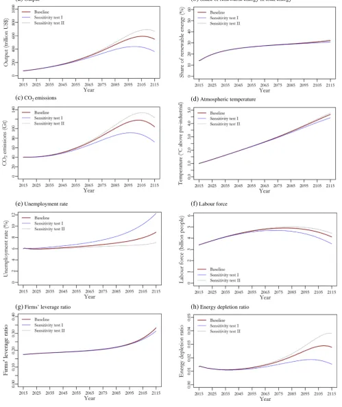
The simulation results are shown inFigs. 2 and 3. In the baseline sce-nario output increases exponentially for about 60 years (Fig. 2a). Since the share of renewable energy in total energy remains low (Fig. 2b), economic growth generates an almost continuous rise in CO2emissions

till the end of the 21st century (Fig. 2c). The resulting rise in CO2

concen-tration and radiative forcing leads to severe global warming: in 2100 at-mospheric temperature becomes 4 °C higher than the pre-industrial levels (Fig. 2d). The rise in atmospheric temperature makes gradually the damage channel stronger. Hence, the growth rate of output declines, becoming very close to 0% at the beginning of the 22nd century. Declin-ing economic growth leads to a gradual rise in the unemployment rate (Fig. 2e).15Low economic activity, combined with the destruction of

capital due to climate change, places upward pressures on the leverage ratio of_ﬁrms (Fig. 2g). The rise in the leverage ratio reinforces the reces-sionary effects caused by global warming (growth channel) because it reduces desired investment and increases credit rationing.Fig. 2f shows the adverse impact that the damages have on the labour force. Remarkably, these damages are not only linked to the effects of global warming; they are also related to the health effects from the accumula-tion of hazardous waste. Two addiaccumula-tional developments are worth men-tioning. First, low economic growth leads ultimately to a reduction in CO2emissions (Fig. 2c). Ironically, this cut is primarily produced by

na-ture–which has forced the economy to slow–and not by any speciﬁc human design. Second, the expansion of the economy and the low use of renewables makes the non-renewable energy sources more scarce via the depletion channel (Fig. 2h).

A crucial question is how these baseline results are modiﬁed when key parameters change or when environmental policies are implement-ed. Although space limitations do not allow us to explore these issues in depth, in what follows we present a sensitivity analysis and two policy scenarios that illuminate the non-neutral impact ofﬁnance on the ecosystem-macroeconomy interactions.

The sensitivity analysis focuses on the effects offirm leverage on economic activity. A rise in the leverage ratio offirms has both con-tractionary and expansionary effects (see alsoNikolaidi, 2014). The contractionary effects stem from the fact that a rise in leverage re-duces desired investment and increases credit rationing. The ex-pansionary effects are basically related to the fact that a rise in firm loans is always accompanied by a rise in household deposits which boosts consumption expenditures via the wealth effect. There are also some effects on the disposable income of households which are less clear-cut: a rise infirm loans increases, on the one hand, the distributed profits of banks and the interest payments of households but, on the other hand, reduces the distributed profits offirms.

Based on the above, we have selected to modify the following pa-rameters in the sensitivity analysis: (i) the sensitivity of the desired in-vestment rate to proﬁtability (a1); (ii) the sensitivity of credit rationing

to the leverage ratio ofﬁrms (r1andl1); (iii) the propensity to consume

out of deposits (c2). In Sensitivity test I,a1,r1andl1are relatively high

andc2is relatively small. This means that the contractionary effects

are strong relative to the expansionary ones. The opposite holds in Sen-sitivity Test II, wherea1,r1andl1are relatively small andc2is relatively

high.Table 5reports the parameter values used in the sensitivity analysis.

Fig. 2shows the results. Under Sensitivity test I, the rise in the lever-age ratio ofﬁrms caused by climate change generates stronger contrac-tionary effects in comparison to the baseline scenario. Hence, output is lower (Fig. 2a) and unemployment rate is higher (Fig. 2e). However, there are beneﬁcial environmental effects. Lower economic activity slows the build-up of atmospheric CO2concentration, resulting in

slightly less severe global warming (Fig. 2d); it also leads to a lower use of the non-renewable energy reserves (Fig. 2h). On the contrary, under Sensitivity Test II, the adverse effects of a higherﬁrm leverage 14

The simulations have been performed using R. The code is available upon request. 15_{The impact of global warming on the unemployment rate depends to a great extent on} the effects of the adaptation measures, which are captured by the parametersadPandadLF.

If the adaptation measures do not limit the damages to labour productivity and labour force sufﬁciently, global warming might lead to a decline in the unemployment rate and might cause labour shortage problems.

(10)

ratio are less pronounced, allowing output to increase more than in the baseline scenario (Fig. 2a). This, of course, increases the environmental problems.

Overall, the results show that the responsiveness of economic activ-ity to the leverage ratio affects the way that the ecosystem interacts with the macroeconomy. In the baseline scenario environmental

(a)

Output

(c)

CO₂emissions

(b)

Share of renewable energy in total energy

(d)

Atmospheric temperature

(e)

Unemployment rate

(f)

Labour force

[image:10.595.46.546.61.656.2]

(g)

Firms’ leverage ratio

(h)

Energy depletion ratio

Fig. 2.Evolution of environmental, macroeconomic andﬁnancial variables, sensitivity analysis (a) Output (b) Share of renewable energy in total energy (c) CO2emissions (d) Atmospheric temperature (e) Unemployment rate (g) Firms' leverage ratio (f) Labour force (h) Energy depletion ratio Note: The values used in the simulation analysis are reported inAppendix A,

(11)

(a)

Output

(c)

CO2 emissions

(b)

Share of renewable energy in total energy

(d)

Atmospheric temperature

(e)

Unemployment rate

(f)

Labour force

[image:11.595.59.553.90.683.2]

(g)

Firms’ leverage ratio

(h)

Energy depletion ratio

Fig. 3.Evolution of environmental, macroeconomic andﬁnancial variables, policy analysis (a) Output (b) Share of renewable energy in total energy (c) CO2emissions (d) Atmospheric temperature (e) Unemployment rate (g) Firms' leverage ratio (f) Labour force (h) Energy depletion ratio Note: The values used in the simulation analysis are reported inAppendix A,

(12)

damages reduce economic growth and destroy capital (via the damage channel), causing a rise in thefinancial fragility offirms (via thefi nan-cial (in)stability channel). This, in turn, harms economic growth (via the growth channel), slowing environmental degradation and the de-pletion of natural resources. When the adverse impact of the leverage ratio on economic activity increases (decreases), the harmful economic effects of environmental damages are amplified (attenuated).

We now turn to analyse a set of policies linked with theﬁnancing conditions for green investment. In our model these conditions are cap-tured by the credit rationing and the interest rate on green loans. An im-provement in the green ﬁnancing conditions means that credit rationing and interest rate on green loans are reduced, leading to a higher share of green investment in total investment. This can be the re-sult of various types of policies, such as a bank regulation policy or a cen-tral bank policy that incentivise banks to provide a higher amount of green loans (seeCampiglio, 2016).

We analyse two types of greenfinance policies. Under Greenfinance policy I, the credit rationing and the interest rate on green loans are re-duced, while the credit rationing and the interest rate on conventional loans remain unchanged. This means that a higher share of green capital in total capital is accompanied by a higher economic growth. The latter partially offsets the beneficial environmental effects of higher green in-vestment. Under greenfinance policy II, the decline in the credit ration-ing and the interest rate on green loans is accompanied by a rise in the credit rationing and the interest rate on conventional loans. This means that the favourable environmental effects of higher green investment are offset to a less extent by higher economic growth caused by credit expansion. Moreover, the share of green capital in total capital becomes even higher.

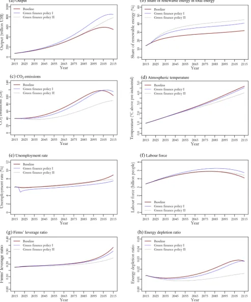
Fig. 3reports the results. The implementation of both policies is as-sumed to start in 2020. As expected, under Greenﬁnance policy I, out-put increases more than in the baseline scenario due to the expansionary effects of higher credit availability and lower interest rates (Fig. 3a); this development is related to the growth channel. Credit expansion also has favourable effects on the unemployment rate (Fig. 3e). The increase in the share of green investment causes a rise in the use of renewable energy (Fig. 3b). Hence, CO2emissions grow less

rapidly compared to the baseline scenario (Fig. 3c), leading to a slightly lower rise in atmospheric temperature. Since global warming is less se-vere, the damage channel is less strong and this allows the economy to expand for a slightly longer period compared to the baseline scenario (Fig. 3a).

Greenfinance policy II yields better environmental results. Since the provision offinance for conventional investment is reduced, economic growth is lower compared to the Green finance policy I scenario (Fig. 3a). The combination of a lower economic activity and a higher share of green investment in total investment generates lower CO2

emissions (Fig. 3c) and, thereby produces a less rapid rise in the atmo-spheric temperature (Fig. 3d).

Particular attention needs to be paid to the trajectory of the leverage ratio offirms (Fig. 3g). Although credit expands significantly under Greenfinance policy I, the leverage ratio turns out to be lower compared to the baseline scenario. The main driving force behind this develop-ment is the enhancedevelop-ment of green investdevelop-ment which reduces the dam-ages (greenfinancing channel), allowing output and capital stock to increase more. Furthermore, when the proportion of green credit in total credit becomes even higher (Greenfinance policy II), the leverage ratio decreases further despite the fact that economic growth is lower than in the Greenfinance policy I scenario. This has to do with the fact that global warming–and hence damages - are less severe when the proportion of green credit increases.

5. Conclusion

This paper developed a stock-flow-fund ecological macroeco-nomic model that analyses the complex interactions between the ecosystem, thefinancial system and the macroeconomy. The foun-dations of the model lie in the post-Keynesian SFC approach and the flow-fund model of Georgescu-Roegen. We calibrated the model using global data and we performed simulations to investi-gate the trajectories of key environmental, macroeconomic andfi -nancial variables under (i) different assumptions about the sensitivity of economic activity to the leverage ratio offirms and (ii) different types of greenfinance policies. Our simulations indi-cated that as the contractionary effects of a higher leverage ratio become stronger, the economic damages caused by the environ-mental changes are reinforced. They also showed that greenfinance policies have favourable effects on environmental variables and the financial fragility offirms. More importantly, these favourable ef-fects are enhanced when the expansion of green credit is accompa-nied by a restriction of conventional credit.

Our analysis can be extended in various directions. First, more real-istic structures can be introduced into our macroeconomy andﬁnancial system. Examples include the incorporation of the equity/bond/energy market, the government sector and the central bank. Second, additional aspects of the ecosystem can be incorporated, such as tipping points or a more sophisticated carbon cycle. Third, various simulation exercises can be conducted–using the current model or its future extensions–in order to explore how our results change when different types of envi-ronmental policies are implemented. All these extensions can contrib-ute to a more integrated understanding of the ways through which macroeconomic andﬁnancial stability can be combined with ecological sustainability.

Table 5

Values of key parameters in the sensitivity and policy analysis.

Parameter

Baseline scenario

Sensitivity test I

Sensitivity test II

Greenﬁnance policy I

Greenﬁnance policy II

Sensitivity of desired investment rate to proﬁtability (α1) 0.2 0.5 0.05 0.2 0.2

Sensitivity of conventional loans' credit rationing to the leverage ratio ofﬁrms (r1) 0.2 0.4 0.05 0.2 0.2 Sensitivity of green loans' credit rationing to the leverage ratio ofﬁrms (l1) 0.2 0.4 0.05 0.2 0.2

Propensity to consume out of deposits (c2) 0.075 0.05 0.1 0.075 0.075

Autonomous desired investment rate (α0) 0.028 0.021 0.032 0.028 0.028

Propensity to consume out of disposable income (c1) 0.88 0.92 0.85 0.88 0.88

Autonomous credit rationing on green loans (l0) 0.37 0.33 0.39 0.27 0.27

Autonomous credit rationing on conventional loans (r0) 0.17 0.13 0.19 0.17 0.37

Interest rate on green loans (intG) 0.08 0.08 0.08 0.06 0.06

Interest rate on conventional loans (intC) 0.07 0.07 0.07 0.07 0.08

(13)

Acknowledgements

We are grateful to Sebastian Berger, Peter Bradley, Vince Daly, Duncan Foley, Ewa Karwowski, Andrew Mearman, Jo Michell, Oliver Richters, Engelbert Stockhammer and Rafael Wildauer for valuable comments. We are also grateful to two anonymous referees for con-structive suggestions. Earlier versions of this paper were presented at the 19th SCEME Seminar in Economic Methodology, Bristol, May 2014, the 18th Conference of the Research Network Macroeconomics and Macroeconomic Policies (FMM), Berlin, October-November

2014, the 25th Annual Workshop of the Post-Keynesian Economics Study Group, London, May 2015, the 11th Conference of the European Society for Ecological Economics, Leeds, June_–July 2015, the Political Economy seminar series of Kingston University, London, December 2015 and the MISUM research seminar series of Stockholm School of Economics, December 2015. We thank the par-ticipants for helpful comments. This research is part of a project con-ducted by the New Economics Foundation. Theﬁnancial support from the Network for Social Change is gratefully acknowledged. The usual disclaimers apply.

Appendix A. Initial values for endogenous variables

Symbol Description Value Remarks/sources

BP Proﬁts of banks (trillion US$) 3.7 Calculated from Eq.(99)using the initial values ofLC,LGandD C Consumption (trillion US$) 47.1 Calculated from Eq.(50)using the initial values ofYandI CEN Carbon mass of the non-renewable energy sources (Gt) 9.8 Calculated from Eq.(7)using the initial value ofEMISIN

CO2AT Atmospheric CO2concentration (Gt) 3,120 Taken from NOAA/ESRL (National Oceanic & Atmospheric Administration/Earth System Research Laboratory)

CO2UP Upper ocean/biosphere CO2concentration (Gt) 5,628.8 Based onNordhaus and Sztorz (2013); Gt of carbon have been transformed into Gt of CO2 CO2LO Lower ocean CO2concentration (Gt) 36,706.7 Based onNordhaus and Sztorz (2013); Gt of carbon have been transformed into Gt of CO2 CONE Amount of non-renewable energy resources converted

in-to non-renewable energy reserves (EJ)

1,626.0 Calculated from Eq.(20)using the initial value ofRESE

CONM Amount of material resources converted into material

reserves (Gt)

194 Calculated from Eq.(12)using the initial value ofRESM

CRC Degree of credit rationing for conventional loans 0.2 Calculated from Eq.(100)using the initial value oflev CRG Degree of credit rationing for green loans 0.4 Calculated from Eq.(101)using the initial value oflev D Deposits (trillion US$) 66.6 Calculated from Eq. (104-red) using the initial value ofL DC Stock of durable consumption goods (trillion US$) 1,185 Calculated from Eq.(4)using the initial values ofK,DEM,δandμ DEM Demolished/discarded socio-economic stock (Gt) 17.0 Based onHaas et al. (2015)

depE Energy depletion ratio 0.013 Calculated from Eq.(22)using the initial values ofENandREVE depM Matter depletion ratio 0.008 Selected from a reasonable range of values

DP Distributed proﬁts ofﬁrms (trillion US$) 6.4 Calculated from Eq.(60)using the initial values ofTPandRP DT Total proportional damage caused by global warming 0.0028 Calculated from Eq.(55)using the initial value ofTAT DTF Part of damage that affects directly the fund-service

resources

0.0026 Calculated from Eq.(57)using the initial values ofDTandDTP

DTP Part of damage that reduces the productivities of

fund-service resources

0.0003 Calculated from Eq.(56)using the initial value ofDT

E Energy necessary for the production of output (EJ) 580.0 Based on IEA (International Energy Agency); total primary energy supply is used ED Dissipated energy (EJ) 580.0 Calculated from Eq.(18)using the initial values ofENandER

EMIS Total CO2emissions (Gt) 40.0 Calculated from Eq.(25)using the initial values ofEMISINandEMISL EMISIN Industrial CO2emissions (Gt) 36.0 Based on CDIAC (Carbon Dioxide Information Analysis Center) EMISL Land-use CO2emissions (Gt) 4.0 Based on CDIAC (Carbon Dioxide Information Analysis Center) EN Energy produced from non-renewable sources (EJ) 498.8 Calculated from Eq.(17)using the initial values ofEandER ER Energy produced from renewable sources (EJ) 81.2 Calculated from Eq.(16)using the initial values ofθandE F Radiative forcing over pre-industrial levels (W/m2

) 2.30 Calculated from Eq.(29)using the initial values ofCO2ATandFEX FEX Radiative forcing, over pre-industrial levels, due to

non-CO2greenhouse gases (W/m2)

0.28 Based onNordhaus and Sztorz (2013)

gLF Growth rate of labour force before global warming

damages

0.012 Based onUnited Nations (2015)

gY Growth rate of output 0.030 Calibrated such that the model generates the baseline scenario described inSection 4 gβ0 Growth rate of the autonomous share of green investment

in total investment

0.001 Calibrated such that the model generates the baseline scenario described inSection 4

gεG Growth rate of green energy intensity −0.050 Calibrated such that the model generates the baseline scenario described inSection 4 gλ Growth rate of labour productivity 0.018 Calculated from Eq.(86)using the initial values of gYandσ0

gμG Growth rate of green material intensity −0.013 Calibrated such that the model generates the baseline scenario described inSection 4 gρG Growth rate of green recycling rate 0.01 Calibrated such that the model generates the baseline scenario described inSection 4 gω Growth rate of CO2intensity −0.005 Calibrated such that the model generates the baseline scenario described inSection 4 hazratio Hazardous waste accumulation ratio (Gt/million km2₎ _0.03 _{Calculated from Eq.}₍₁₀₎_{using the initial value of}_HWS

HWS Stock of hazardous waste (Gt) 14.0 Calculated assuming a constant ratio of hazardous waste to GDP since 1960 I Total investment (trillion US$) 26.1 Calibrated such that the model generates the baseline scenario described inSection 4 IC Conventional investment (trillion US$) 15.7 Calculated from Eq.(77)using the initial values ofIandIG

ICD Desired conventional investment (trillion US$) 17.5 Calculated from Eq.(69)using the initial values ofIDandIGD ID

Desired total investment (trillion US$) 31.3 Selected such that it is reasonably higher thanI

IG Green investment (trillion US$) 10.4 Calculated by assuming thatIG/Iis slightly lower thanβ; the initial values ofβandIare used IGD Desired green investment (trillion US$) 13.8 Calculated from Eq.(68)using the initial values ofβandID

K Total capital stock (trillion US$) 380.6 Calculated from the identityK= (K/Y)∗Yby using the initial value ofYand assuming thatK/Y = 5.2 (this value has been selected such that the model generates the baseline scenario described inSection 4)

KC Conventional capital stock (trillion US$) 290.3 Calculated from Eq.(81)using the initial values ofKandKG