Stochastic domain decomposition for time dependent adaptive mesh generation

Stochastic Domain Decomposition for Time

Dependent Adaptive Mesh Generation

Alexander Bihlo1,2, Ronald D. Haynes1,∗, Emily J. Walsh3

1_{Department of Mathematics and Statistics, Memorial University of Newfoundland,} St. John’s (NL), A1C 5S7, Canada.

2_{Department of Mathematics, University of British Columbia Vancouver (BC), V6T} 1Z2, Canada.

3_{Department of Engineering Design and Mathematics, University of Western} Eng-land, Bristol BS16 1QY, United Kingdom

Received 1 April, 2015; Accepted (in revised version) 22 May, 2015

Abstract. The efficient generation of meshes is an important component in the numer-ical solution of problems in physics and engineering. Of interest are situations where global mesh quality and a tight coupling to the solution of the physical partial dif-ferential equation (PDE) is important. We consider parabolic PDE mesh generation and present a method for the construction of adaptive meshes in two spatial dimen-sions using stochastic domain decomposition that is suitable for an implementation in a multi– or many–core environment. Methods for mesh generation on periodic do-mains are also provided. The mesh generator is coupled to a time dependent physical PDE and the system is evolved using an alternating solution procedure. The method uses the stochastic representation of the exact solution of a parabolic linear mesh gen-erator to find the location of an adaptive mesh along the (artificial) subdomain in-terfaces. The deterministic evaluation of the mesh over each subdomain can then be obtained completely independently using the probabilistically computed solutions as boundary conditions. A small scaling study is provided to demonstrate the parallel performance of this stochastic domain decomposition approach to mesh generation. We demonstrate the approach numerically and compare the mesh obtained with the corresponding single domain mesh using a representative mesh quality measure.

AMS subject classifications: 65N50, 65M50, 65L50, 65C05,65N55, 65M55

Key words: Mesh generation, Domain decomposition, Monte Carlo methods.

1

Introduction

The numerical solution of many partial differential equations (PDEs) benefits from the construction of an adaptive grid automatically tuned by the solution itself. The quasi–

∗_{Corresponding author. Email addresses: [email protected] (A. Bihlo), [email protected] (R. D. Haynes),} [email protected](E. J. Walsh)

Lagrangian (QL),r–refinement, approach used here keeps the number of mesh points and the mesh topology fixed, moving the mesh continuously in time using a moving mesh PDE (MMPDE). The solution of the mesh PDE gives a continuous mesh transformation between an underlying computational co-ordinate and the required physical co-ordinate. Both the mesh and the solution are obtained at each time step. The QL approach can be implemented in either an alternating or simultaneous manner. The simultaneous QL approach treats the MMPDE and physical PDE as one large coupled system. At each time the new mesh and new solution on that mesh are found concurrently. Hence the mesh reacts instantly to changes in the physical solution. This highly nonlinear coupling may destroy exploitable structure which exists in the discretization of the physical PDE alone. The alternating approach uses the current mesh and physical solution to update the mesh alone, this new mesh then facilitates the computation of the updated physical solution. This introduces a time lag in the mesh as the new mesh is based only on the current physical solution. Computationally, however, this decoupling reduces the size of the discrete problem. Furthermore, the solver becomes more modular; the mesh and physical solvers can be called in alternating fashion; each solver can be designed to take advantage of the structure inherent in each subsystem. The simultaneous approach is generally thought to be more difficult and expensive to solve and hence the alternating method (or a variant thereof) is typically used in two or more spatial dimensions. As we will see below, the alternating approach fits well with the stochastic domain decomposition approach we describe to parallelize our computations.

The general QL approach has shown great promise in recent years, solving problems in meteorology [7], relativistic magnetohydrodynamics [14], combustion and convection in a porous medium [9], groundwater flow and transport of nonaqueous phase liquids [16], Stefan problems [4], semiconductor devices [30], and viscoelastic flows [31], phase change problems [3], multiphase flows [26], and low speed viscous flow [18], to name just a few. A thorough overview of PDE based moving mesh methods may be found in [15].

Recently, motivated by the alternating solution method, one of the authors has stud-ied the parallel solution of the nonlinear MMPDE alone using a Schwarz based domain decomposition approach. In [12], Haynes and Gander propose and analyze classical, optimal and optimized Schwarz methods in one spatial dimension at the continuous level. A numerical study of classical and optimized Schwarz domain decomposition for 2D nonlinear mesh generation has been presented in [13]. In [10], amonolithic domain decomposition method, simultaneously solving a linear mesh generator coupled to the physical PDE, was presented for a shape optimization problem. The authors used an overlapping domain decomposition approach to solve the coupled problem.

In this paper, we present an efficient, parallel strategy for the solution of the moving mesh PDE based on a stochastic domain decomposition method proposed by Acebr ´on

quality, not an extremely accurate solution of the mesh PDE, which is important. As we will see, the stochastic domain decomposition approach is a means to these ends.

A stochastic domain decomposition (SDD) method to find adaptive meshes for steady state elliptic problems was presented in [5]. The SDD approach, as originally formulated in [1], uses a probabilistic form of the point–wise solution for linear elliptic boundary value problems. The point–wise solution is evaluated only at the introduced subdomain interfaces. The approximation of the solution at each interface point is obtained indepen-dently using Monte–Carlo simulations and these evaluations are then used as Dirichlet boundary conditions for the (deterministic) subdomain solves which can be computed in parallel. The mesh PDEs are generally not solved to high accuracy. Mesh quality, al-lowing an accurate representation of the physical PDE, is what is generally required. The parallel algorithm and lower accuracy requirement makes the proposed SDD method computationally attractive. The lower accuracy requirement allows one to terminate the Monte–Carlo simulations well before convergence.

The existence of a stochastic representation of the exact solution of linear parabolic problems allowed us to extend the SDD approach to (linear) parabolic mesh generators in [5]. There we considered the time relaxed form of the Winslow–Crowley variable dif-fusion mesh generation method, first described in [29]. Only the solution of the mesh generator for a specified analytic mesh density function was considered.

Here we consider the generation of time dependent meshes where the mesh PDE is coupled to a physical PDE of interest. The coupling to the physical solution u, is pro-vided by, for example, an arc-length type function ρ=

q

1+α(u2_x+u2_y). The parameter

αis chosen to provide a balanced coupling with the physical PDE. Furthermore, due to

a stochastic representation for the solution of PDEs subject to periodic boundary con-ditions, we give, for the first time, a method to generate meshes for periodic problems using a stochastic domain decomposition approach.

2

Mesh generation approach

As discussed extensively in the references above, in 1D the QL r–refinement approach generates a physical meshx∈[0,1], via a continuous mesh transformation x(ξ), where ξ∈[0,1]is an underlying computational variable. A guiding principle is the

equidistri-bution principle of de Boor (in 1D) [8, 11, 28], which finds a mesh transformationx(ξ)by

enforcing

Z _ξ

0 ρ

(t,u, ˜x)dx˜=ξ Z 1

0 ρ

(t,u, ˜x)dx˜,

where the mesh density functionρgives a measure of the level of difficulty or error in the

physical solutionu. The physical solutionumay be given analytically or as the solution of a physical PDE. In differential form, the mesh transformation may be found as the solution of the quasilinear BVP

d dξ

ρ(x)dx

dξ

=0, x(0) =a,x(1) =b. (2.1)

Here we have suppressed the t and u dependency in ρ. This gives the physical co–

ordinates xi=x(ξi) as a function of a (typically uniform) computational grid ξi. This

BVP can be written as a linear BVP in terms of the inverse mesh transformationξ(x)as

d dx

1

ρ(x)

dξ

dx

=0, ξ(a) =0,ξ(b) =1. (2.2)

The linearity of the BVP forξ(x)makes it easier to solve (in some sense) and in higher

dimensions has the additional benefit that it is easy to say concrete things about the well– posedness of the mesh transformation. As will be discussed below, the linearity of a mesh generator is also a prerequisite for the stochastic domain decomposition method. The obvious disadvantage is that the solution of the BVP forξ(x)does not give the mesh

lo-cations in the physical variablesx. One alternative is to transform the physical PDE from the physical variables to the new computational co-oordinates. Alternatively, inverse lin-ear interpolation could be used to find thexlocations by projectingξ(x)onto a uniform ξ grid.

Indeed, in [5] we constructed our stochastic DD method for steady state mesh gener-ation using the natural 2D extension of the linear BVP (2.2). In the time dependent case considered in this paper we will construct a stochastic DD method directly in the physi-cal co-ordinates. The time stepping will provide a natural linearization as we will show below.

A natural way to derive the BVPs above (and which extends to higher dimensions) is as the Euler–Lagrange equations whose solutions minimize certain functionals of the required mesh transformations. For example minimizing the functional

I[x] =1

2

Z 1

0

ρ(x)dx

dξ 2

leads to the quasi–linear BVP (2.1) above. A minimizerξ(x)of the functional

I[ξ] =1

2

Z b

a

1

ρ(x)

dξ

dx

2

dx

satisfies the linear BVP (2.2) above.

For time dependent PDEs it is useful to use a formulation which involves the mesh speed, such a mesh equation is called a moving mesh PDE (MMPDE). If ρ=ρ(t,x) the

functionalI[ξ]becomes

I[ξ] =1

2

Z b

a

1

ρ(t,x)

dξ

dx

2

dx.

As described in [15], the direction ξ which reduces I[ξ] is given by the gradient flow

equation dξ dt= P τ d dx 1

ρ(t,x)

dξ

dx

,

where τ>0 is a user specified constant which determines the response of the mesh to

changes inρ(oru). HerePis a positive definite differential operator that we choose with

some flexibility.

We can switch the roles ofxandξ in the gradient flow equation to get a

mathemati-cally equivalent moving mesh PDE in the physical variablesx:

∂x

∂t =

1

τ ∂x

∂ξP

ρ∂x ∂ξ −2 ∂x ∂ξ −1 ∂ ∂ξ

ρ∂x ∂ξ

.

Hence this resulting equation would retain the nice well–posedness properties. If we chooseP= (ρxξ)2, then we get

∂x

∂t =

1

τ ∂

∂ξ

ρ∂x ∂ξ

, (2.3)

which is referred to as MMPDE5. Our focus here is the generation of time dependent meshes by using this nonlinear parabolic mesh generator.

The coupling to the physical PDE and physical solution uis provided by the mesh density functionρ(x,u). In a typical deterministic implementation, the mesh and physical

solution are updated by discretizing MMPDE5 and the physical PDE in time and either solving the resulting large nonlinear system of algebraic equations for both the mesh and physical solution simultaneously or proceeding in an alternating fashion. The alternating or MP approach [15] used in this paper freezesρin the time discretized mesh equation at

the currentunto compute the next meshxn+1_{and then integrates the physical PDE, using}

In two spatial dimensions we use the mesh generator

xt=

∇_ξρ

ρ ·∇ξx+∇

2

ξx, yt=

∇_ξρ

ρ ·∇ξy+∇

2

ξy,

x(0,ξ) =x0=Lxξ, y(0,ξ) =y0=Lyη,

(2.4)

whereξ= (ξ,η)and∇ξ= (∂/∂ξ,∂/∂η), which we solve over the square computational

domainΩc=[0,1]×[0,1]. For the sake of simplicity we assume a rectangular domainΩp= [0,Lx]×[0,Ly], whereLx>0,Ly>0. At the actual boundaries of the computational domain Ωc, we employ the fixed boundary conditionsx(t,0,η) =0,x(t,1,η) =Lx,y(t,ξ,0) =0 and

y(t,ξ,1)=Ly. The remaining boundary conditions,x(t,ξ,0),x(t,ξ,1),y(t,0,η)andy(t,1,η)

are found by solving the respective one-dimensional forms of the mesh generator (2.4) along these boundaries.

Note that the mesh generator (2.4) is obtained byfirstdividing the two dimensional version of (2.1) by ρ and then relaxing the equation in time. We have found in

prac-tice that this form of a relaxed mesh generator gives better meshes than by relaxing the original version (2.1). In the discrete formulation, these two possible time relaxed mesh generators are related by a scaled time step.

We are also interested in mesh generation on periodic domains. It has been pointed out in [27], that in order to use the mesh generator (2.4) on a rectangular periodic domain of physical dimensionsΩp=0,Lx[×[0,Ly[,

x(t,1,η) =x(t,0,η)+Lx, y(t,ξ,1) =y(t,ξ,0)+Ly,

one should express the mesh and physical PDEs in terms of the displacementsX=x−Lξ,

whereL=diag(Lx,Ly),x= (x,y)andX= (X,Y), which are directly periodic onΩc. In this

new set of variables, the mesh generator (2.4) becomes

Xt=

∇_ξρ

ρ ·∇ξX+∇

2

ξX+ ρξ

ρ (1+Lx), Yt=

∇_ξρ

ρ ·∇ξY+∇

2

ξY+ ρη

ρ (1+Ly).

An alternative to the procedure proposed in [27] works directly in the original vari-ablesxandyand properly extends the computational domain using the periodicity of the grid. This allows one to evaluate the derivatives ofxon the boundaries without having to take into account the actual size of the physical domainΩp. As this approach allows

one to work with the physical coordinatesxdirectly, we use this second method in this paper.

3

Stochastic domain decomposition and mesh generation

3.1 Stochastic domain decomposition for linear PDEs

The main idea of stochastic domain decomposition as proposed in [1] (see also [2]) rests on the stochastic representation of the exact solution to linear elliptic (resp. parabolic)

boundary value problems. This now classical connection between stochastic analysis and boundary value problems was first uncovered by Kakutani [19,20] for the Dirichlet prob-lem using Brownian motion. The monographs [21, 24] provide a more recent exposition.

Numerically evaluating this stochastic representation of the exact solution of a linear boundary value problem using Monte–Carlo methods enables one to compute the point-wise numerical solution to the underlying PDE. From the practical point of view, this is fundamentally different to solving a PDE using, say, finite differences, which requires the computation of the numerical solution over the entire domain even if it is only needed in a single point.

Notoriously, Monte–Carlo methods converge slowly, with convergence rates propor-tional to N−1/2 where N is the number of Monte–Carlo simulations, if pseudo-random numbers are used [25]. Hence they play a role mostly for higher dimensional problems, where they can be shown to outperform deterministic methods.

An alternative is to use them in the context of domain decomposition. Namely, split-ting the entire domain into non-overlapping subdomains, the stochastic solution can be used to compute the point-wise interface solutions between the subdomains. Once these interface solutions are determined with sufficient accuracy, they act as Dirichlet bound-ary values for the individual subdomains. The PDE solution over each subdomain is computed deterministically using an appropriate discretization of the underlying PDE. The main advantage of this method is that iteration, as is required in classical domain decomposition methods (such as Schwarz methods), can be completely avoided. Also, the solutions over each subdomain can be obtained in parallel and thus the method is suitable for massively parallel computing architectures.

In [5, 6] we have shown that the stochastic domain decomposition technique is an effective way for the parallel generation of adaptive meshes. A main motivator for the approach is that it is, in general, not necessary to compute the meshes with high accuracy. What is important is to obtain meshes with high mesh quality. It was shown in [5, 6] that even meshes that are not accurate solutions to the mesh PDEs can have good mesh quality. This characteristic of mesh generation enables an increase in the efficiency of the stochastic domain decomposition method.

3.2 Stochastic analysis for Dirichlet boundary value problems

In this section we give the specifics of the stochastic analysis required to generate the solution of linear parabolic boundary value problems. Specifically, we consider system (2.4) where the unknowns x=x(t,ξ,η) andy=y(t,ξ,η)are required on the time-space

domain given by [0,T]×Ωc, withT being some finite final time. System (2.4) is

for given continuous functions f and g. The initial values are x(0,ξ,η) =x0(ξ,η) and

y(0,ξ,η) =y0(ξ,η).

It is important to stress here that (2.4) is nonlinear if the mesh density function is a function on the physical domain, that is ρ=ρ(t,x,y). However, as was indicated in

Section 2, in the practical implementation it is possible to freezeρat time layertnwhen

computing the mesh at time tn+1. This effectively boils down to a linearization of the mesh generator (2.4). It is thus appropriate to assume thatρin (2.4) is not a function ofx

andybut of some auxiliary variables ˜xand ˜y(and time), i.e. we assume thatρ=ρ(t, ˜x, ˜y).

Then this mesh generator becomes linear and allows for a stochastic representation of its exact solution [23], given by

x(t,ξ,η) =E h

x0(Φ(t))1[τ_∂Ωc>t]

i

+Ehf(t−τ_∂Ωc,Φ(τ_∂Ωc))1[_τ∂Ω c<t]

i

,

y(t,ξ,η) =E h

y0(Φ(t))1[τ∂Ωc>t] i

+Ehg(t−τ∂Ωc,Φ(τ∂Ωc))1[τ∂Ωc<t] i

,

(3.1a)

where the stochastic processΦ(t)satisfies the stochastic differential equation (SDE)

dΦ(t) =1

ρ∇ξρdt+

√

2dW(t). (3.1b)

In (3.1), E[·]is the expected value,τ∂Ωcis the first exit time of the stochastic processΦ(t)

starting at(ξ,η),Wis two-dimensional Brownian motion and1is the indicator function.

See [21, 23, 24] for a more extensive discussion of this subject. We note that the stochastic solution (3.1a) has contributions from both the specific initial condition and boundary values of the mesh generator.

3.3 Stochastic analysis for periodic problems

Freezing ρ the mesh generator (2.4) is in the form of a system of linear, second order,

parabolic PDEs. In Section 3.2 we wrote the stochastic point–wise solution assuming a Dirichlet boundary value problem. On periodic domains, the celebrated Kac–Feynman formula can be used to obtain the stochastic representation of the mesh generator (2.4), see e.g. [23]. In this case, only initial valuesx(0,ξ,η) =x0(ξ,η)andy(0,ξ,η) =y0(ξ,η)are

given. The solution to (2.4) can then be written as

x(t,ξ,η) =E[x0(Φ)], y(t,ξ,η) =E[y0(Φ)], (3.2)

whereΦsatisfies the same stochastic differential equation as given in (3.1b).

3.4 Stochastic domain decomposition on periodic and non-periodic domains

more complicated. The mesh density functionρis linked to the solution of the physical

PDE system, which changes over time. For this reason, in practice we use (3.1) and (3.2) only to advance the mesh over a single time step,∆t, fromtntotn+1.

We discretize the SDE (3.1b) using the Euler–Maruyama method,

Φk+1_=Φk₊∇ξρ ρ

(tn_,Φk₎∆

ts+p2∆tsW(0,1), (3.3)

with constant time step∆ts=∆t/M,k=0,...,M−1, whereWis a two-dimensional vector

of Gaussian distributed random numbers with zero mean and variance one. In other words, one time step of size∆tis split intoMsub-time steps. This splitting is necessary so that the use of an excessively small time step∆tfor the solution of the physical differential equation can be avoided. The mesh density functionρremains fixed at time steptn. The

derivatives∇_ξρare approximated with finite differences.

In practice, the starting points of the stochastic process at timetn_,Φ0_{, coincide with}

the grid points where the stochastic solution is required. Once the new values Φk+1 at time tk+1 are computed, both ρ and ∇ξρ have to be approximated at Φk

+1_{. For this,}

bi-linear interpolation is used. The procedure is repeated until ΦM is computed, which coincides with the value of the stochastic process at time tn+1_{. We then evaluate the}

initial values ofx0andy0given at timetnat the new locationΦMusing bi-cubic

interpo-lation. This gives the values ˜x0(ΦM)and ˜y0(ΦM), which approximate the actual values x0(Φn+1) andy0(Φn+1) that are needed in both the solutions (3.1a) (for the first term)

and (3.2).

Solving Dirichlet boundary value problems stochastically, a boundary test has to be applied to determine whether the processΦk+1 has left the domain within the sub-time step [tk,tk+1_{]. A linear Brownian bridge is used as interpolating process as discussed}

in [17]. If the process left the domain before timetn+1, the integration can be stopped and the second term in (3.1a) can be evaluated. No such boundary test is needed for periodic domains.

In order to estimate the expected value using the arithmetic mean, the procedure is repeatedNtimes.

3.5 Local subdomain problem

In the domain decomposition solution to the problem (2.4), we only use the stochastic solutions (3.1) and (3.2) to generate the subdomain interface solutions for the Dirichlet and periodic problems. Once these solutions are computed, the solution to the mesh generation problem on the individual subdomains becomes a Dirichlet boundary value problem. In order to solve this problem, the original parabolic mesh generator (2.4) has to be solved with the Dirichlet boundary conditions

x|_∂Ωi

where∂Ωi_cdenotes the boundary of thei–th subdomain of the computational domain and

fi are the values obtained either from the stochastic representation (3.1) or the boundary conditions on the global mesh where∂Ωi_cT∂Ωc6=∅.

For the local subdomain solver we discretize (2.4) using centered finite differences for the spatial derivatives and an implicit Euler method for the time stepping.

3.6 Domain decomposition solution

The domain decomposition strategy relies on combining the stochastic evaluation along the interfaces with the deterministic subdomain solver. At each time step, the stochas-tic solution procedure provides the Dirichlet boundary conditions for the determinisstochas-tic single-domain solver. This allows the computation of the new mesh at the time steptn+1. The solution values can either be evaluated stochastically at each(ξi,ηj)along the

artifi-cial interfaces or a sample can be evaluated with the rest obtained by interpolation. An optimal placement strategy for the interpolation nodes was presented in [5].

Once the new mesh is computed, the mesh density functionρ(tn+1,x,y)is evaluated

on the new mesh and the solution procedure is repeated with the new mesh density function.

3.7 Mesh quality

As mentioned previously, there is a crucial difference between the SDD method as pro-posed in [1] for the computation of numerical solutions of general linear elliptic boundary value problems and for the mesh generation case. The latter does not necessarily require a very accurate solution of the mesh equation; here, mesh quality is more important.

There are several ways of assessing the quality of an adaptive mesh and different mesh quality measures based on properties such as equidistribution and alignment have been derived. See [15] for an extensive discussion of mesh quality measures. In [5] it was proposed to use the geometric mesh quality measure for the assessment of the quality of meshes generated using the SDD method. The geometric mesh quality measure is defined by

Q(K) =1

2

tr(JT_J)

p

det(JT_J), (3.4)

whereJis the Jacobian of the transformationx=x(ξ,η),y=y(ξ,η)andKis a mesh element

inΩc. The quantityQ(K)measures how far the mesh cell is from being equilateral, that

is we haveQ(K)≥1 withQ(K) =1 precisely for an equilateral cell.

the mesh density function used and the underlying problem for which an adaptive grid is computed. We are therefore not interested in the absolute value of Q(K)but only in the ratio betweenQSD(K), the geometric mesh quality measure of the reference mesh ob-tained on a single domain, andQSDD_{(K), the geometric mesh quality measure of the grid}

obtained using the SDD method. If this ratioR(K) =QSD/QSDDis close to one, the mesh obtained from the SDD method is a good approximation to the single domain mesh.

The quantityRis a function of each individual mesh cell. In the next section, for the sake of convenience, we only list the maximum and mean values, Rmax andRmean over

all mesh cells.

4

Numerical results

In this section, numerical experiments in 2D are presented to demonstrate the effective-ness of the domain decomposition algorithm and its suitability for problems with both Dirichlet and periodic boundary conditions.

4.1 Burgers’ equation with Dirichlet boundary conditions

The first test problem considered is the scalar form of the two-dimensional Burgers’ equa-tion

ut+(u2/2)x+(u2/2)y+ν(uxx+uyy) =0, (4.1)

[x,y]∈Ωp= [0,1]×[0,1]. The initial and Dirichlet boundary conditions are chosen such that the exact solution is

u=

1+exp

x+y−t0

2ν

−1

,

and we consider the case of a moderately small diffusion coefficient ν=0.005. In this

problem the smallerν, the more convection dominates, and large gradients develop and

move to the boundaries fort>0, thus requiring a higher concentration of mesh points to resolve the oblique shock that propagates with time. This is a common test problem in the moving mesh literature [22,32]. The coordinate transformation(x,y) = (x(ξ,t),y(ξ,t))

is used to rewrite the 2D Burgers’ equation in QL form in computational coordinates, and this is discretized in the computational domain using centered differences in space and a trapezoidal rule for the time integration. This is coupled to the mesh generator (2.4). Both (2.4) and (4.1) are then solved alternately in time (the MP procedure) for each subdomain using an arc-length mesh density function

ρ= q

1+α(u2_x+u2_y),

withα=10/ku2_x+u2_yk_∞. The Dirichlet boundary conditions (at the subdomain interfaces)

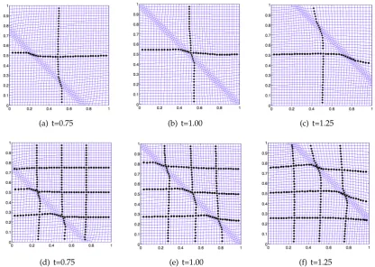
(a) t=0.75 (b) t=1.00 (c) t=1.25

(d) t=0.75 (e) t=1.00 (f) t=1.25

Figure 1: Evolution of mesh for Burgers’ equation using the stochastic DD method with2×2(top) and4×4

(bottom) subdomains.

is solved. We integrate the finite difference discretization of (4.1) using 41×41 grid points on the physical domainΩc= [0,1]×[0,1]with a time step∆t=0.001. The initial time is t0=0.25. We useN=10000 Monte–Carlo simulations with a time step∆ts=∆t/10 for the

solution of the stochastic differential equation (3.3). In Fig. 1 the evolution of the mesh is shown when the physical domain is split into 2×2 and 4×4 subdomains.

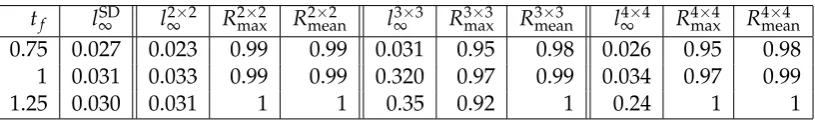
We report the mesh qualities and the l_∞-norm comparing the exact solution to the numerical solution at timestf=0.75,tf=1 andtf =1.25 in Table 1. The geometric mesh

quality measure is computed for the single domain solution and compared to the DD solution obtained by splitting the physical domain into 2×2, 3×3 and 4×4 subdomains.

Table 1: Mesh quality andl_∞-errors for Burgers’ equation with Dirichlet boundary conditions.

tf lSD_∞ l_∞2×2 Rmax2×2 R2mean×2 l3∞×3 R3max×3 R3mean×3 l∞4×4 R4max×4 R4mean×4

0.75 0.027 0.023 0.99 0.99 0.031 0.95 0.98 0.026 0.95 0.98 1 0.031 0.033 0.99 0.99 0.320 0.97 0.99 0.034 0.97 0.99 1.25 0.030 0.031 1 1 0.35 0.92 1 0.24 1 1

The scaling properties of the SDD algorithm are reported in Table 2. For this study we solved Burgers’ equation with Dirichlet boundary conditions on a varying number of subdomains, including 2×2, 4×4, 8×8 and 16×16 subdomains. Three series of experi-ments with a total ofN×N=81×81,N×N=97×97 andN×N=113×113 points covering the physical domain were carried out.

Table 2: Time in seconds required per time step to construct the mesh for Burgers’ equation with Dirichlet boundary conditions.

N_total×N_total SD 2×2 4×4 8×8 16×16 81×81 0.22 0.45 0.33 0.24 0.12 97×97 0.34 0.56 0.40 0.27 0.16 113×113 0.84 0.68 0.51 0.35 0.17

It can be seen from Table 2 that increasing the number of processors (and thus the number of subdomains) indeed leads to a decreased computational time per time step required to construct the adaptive mesh. For a total of N×N=81×81 mesh points, the solution on 16×16 subdomains is computationally cheaper than the single domain so-lution. Increasing the number of total points to N×N=97×97 makes both the solution on 8×8 and 16×16 subdomains cheaper compared to the single domain solution. If

N×N=113×113 total points are used, the domain decomposition solution is computa-tionally faster than the single domain solution for all numbers of subdomains.

The results of Table 2 thus demonstrate the potential of the stochastic domain de-composition algorithm to be significantly more efficient in generating adaptive meshes for problems with a large number of total points provided that enough parallel compute cores are available.

4.2 Periodic mesh generation

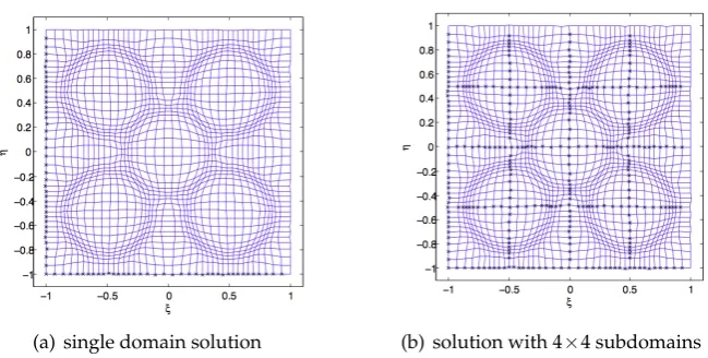
(a) single domain solution (b) solution with 4×4 subdomains

Figure 2: A comparison of the single domain mesh and the mesh obtained for4×4subdomains for the five ring problem.

velocity function of the form

u=tanh

R

x2+y2−1

8 +tanh " R

x−1

2

2

+

y−1

2 2 −1 8 !# +tanh " R

x−1

2

2

+

y+1

2 2 −1 8 !# +tanh " R

x+1

2

2

+

y−1

2 2 −1 8 !# +tanh " R

x+1

2

2

+

y+1

2 2 −1 8 !# ,

on the domainΩp= [−1,1[×[−1,1[, withR=30. A simple arc-length mesh density

func-tion

ρ= q

1+α(u2_x+u2_y),

withα=0.2 is used. The physical domain is discretized using 41×41 grid points, the final

integration time ist=0.05 with a time step∆t=5×10−4. Since this time step is quite small, we use ∆ts=∆t for the solution of the discretized SDE (3.3) as well. Again, N=10000

Monte–Carlo simulations were used. In Fig. 2 the mesh generated on a single domain is compared to the mesh generated by splitting the physical domain into 4×4 subdomains.

4.3 Burgers’ equation on a periodic domain

We repeat here the integration of Burgers’ equation (4.1) but now using a doubly periodic domain of sizeΩp= [0,2π[×[0,2π[. The initial condition is

u=u0+Asin(x+y−2π),

where u0=0.75 and A=0.5. The diffusion coefficient is ν=0.001. Again, 41×41 grid

points are used and the time step of the integration was∆t=0.005, which coincides with the time step used in the SDE (3.3). Only N=1000 Monte–Carlo simulations were used. The results of the integration at timest=0.85 andt=1 are collected in Table 3.

Table 3: Mesh qualities for Burgers’ equation with periodic boundary conditions.

tf R2max×2 R2mean×2 Rmax3×3 R3mean×3 Rmax4×4 R4mean×4

0.85 0.99 1 1 1 0.99 1

1 0.99 1 0.99 1 0.99 1

The results in Table 3 confirm that the domain decomposition solution leads to meshes with almost the same geometric mesh quality as the single domain reference solution.

4.4 Shallow water equations on a periodic domain

In this final example we solve the system of shallow-water equations in nondimensional form

ut+uux+vuy+hx=0,

vt+uvx+vvy+hy=0,

ht+uhx+vhy+h(ux+vy) =0,

(4.2)

where (u,v)is the two-dimensional velocity field and his the height of a water column over a constant reference level. For this problem, periodic boundary conditions are con-sidered.

We discretize system (4.2) in computational coordinates using centered differences for the spatial derivatives and a trapezoidal rule for the time integration. The physical domain is of sizeΩp= [0,2π[×[0,2π[, which is discretized using 41×41 grid points. The

time step of the integration was∆t=0.005, which again coincides with the time step used for the solution of the SDE (3.3). We found that using N=1000 Monte–Carlo simulations gives sufficiently good results.

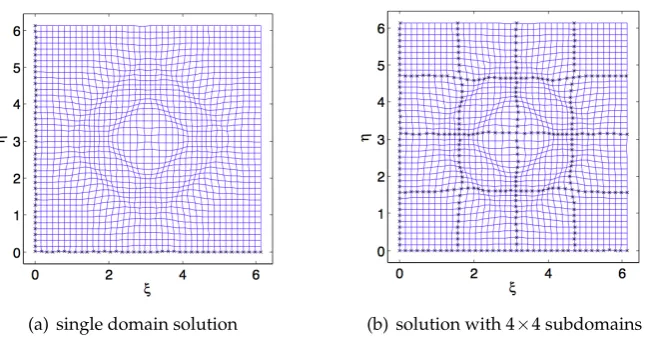
(a) single domain solution (b) solution with 4×4 subdomains

Figure 3: A comparison of the single domain solution and that obtained for4×4subdomains for the shallow water equations att=0.15.

Since the initial pile of water decays rapidly into gravity waves, we kept the inte-gration times short and report our mesh quality results only at t=0.05 andt=0.15. A comparison of the mesh for the single domain solution and that computed for 4×4 sub-domains can be seen in Fig. 3.

As we saw in the previous examples the meshes appear to be of similar quality and this is substantiated by the computed mesh quality measures which can be found in Table 4. The mesh qualities obtained from the domain decomposition solution are very close to that of the single domain reference solution.

Table 4: Mesh quality for the shallow-water equations with periodic boundary conditions.

t_f R2×2

max R2mean×2 R3max×3 Rmean3×3 R4max×4 R4mean×4

0.05 0.99 1 0.97 1 0.99 1 0.15 0.99 1 0.99 1 0.99 1

5

Conclusion

Originally, the SDD method has been proposed in [1] for the parallel solution of linear elliptic boundary value problems. In [5, 6] we have extended the method to the parallel generation of adaptive meshes for prescribed mesh density functions. In this paper we have for the first time demonstrated the use of stochastic domain decomposition for the generation of adaptive moving meshes for time dependent PDE problems. Furthermore, we have provided the first stochastic domain decomposition method for the generation of meshes on periodic domains.

Indeed the linearization provided by the MP procedure has the undesirable affect of decoupling the physical solution from the mesh. This effect can be reduced using aMkP

procedure. This produces a mesh which more closely satisfies the equidistribution princi-ple. In this case, we approximatexn+1_{by a sequence ofsub-meshes x}n+1,k_{, wherex}n+1,k+1

is obtained fromxn+1,k by using a step of∆tn/Kwith a linearized MMPDE. In this case ρ is approximated by ρn+1,k obtained by constructing a piecewise linear interpolant of

(xn_,ρn_{)values onto x}n+1,k_{. AM}ν_{Palgorithm, which updates fromt}

ntotn+1using

vari-able time steps can also be used. The time lag between the mesh and physical solution can be reduced by iterating between the mesh and physical PDE ltimes, resulting in a

(MP)l _{algorithm. The algorithm (MP)}∞ _{is equivalent to the simultaneous solution (if}

the iteration converges). These solution variants are discussed at length in [15]. The im-plementation of these variants and a study of their efficacy within the stochastic domain decomposition framework is a topic of current investigation.

During our experiments we also detected that fewer Monte–Carlo simulations are needed to generate quality periodic meshes. This seems to be due to the absence of an exit time test for the periodic case. Work to fully understand and utilize this is also underway.

Acknowledgements

The authors thank Weizhang Huang for helpful discussions. AB is a recipient of an APART Fellowship of the Austrian Academy of Sciences. This research was supported by the Natural Sciences and Engineering Research Council of Canada (NSERC).

References

[1] J. A. Acebr ´on, M. P. Busico, P. Lanucara and R. Spigler. Domain decomposition solution of elliptic boundary-value problems via Monte Carlo and quasi-Monte Carlo methods. SIAM J. Sci. Comput., 27: 440–457, 2005.

[2] J. A. Acebr ´on and R. Spigler. A new probabilistic approach to the domain decomposition method. In Domain Decomposition Methods in Science and Engineering XVI, Springer, Berlin Heidelberg, 473–480, 2007.

[3] M. J. Baines, M. E. Hubbard, P. K. Jimack and R. Mahmood. A moving-mesh finite element method and its application to the numerical solution of phase-change problems. Commun. Comput. Phys. 6: 595–624, 2009.

[4] G. Beckett, J. A. Mackenzie and M. L. Robertson. A moving mesh finite element method for the solution of two-dimensional stefan problems. J. Comput. Phys. 168: 500–518, 2001. [5] A. Bihlo and R. D. Haynes. Parallel stochastic methods for PDE based grid generation.

Com-put. Math. Appl. 68: 804–820, 2014.

[6] A. Bihlo and R. D. Haynes. A stochastic domain decomposition method for time depen-dent mesh generation. In Domain Decomposition Methods in Science and Engineering XXII, Springer, in press, 2015.

[8] H. G. Burchard. Splines (with optimal knots) are better. Appl. Anal. 3: 309–319, 1974. [9] W. Cao, W. Huang and R. D. Russell. Anr-adaptive finite element method based upon

mov-ing mesh PDEs. J. Comput. Phys., 149: 221–244, 1999.

[10] R. Chen and X. C. Cai. Parallel One-Shot Lagrange-Newton-Krylov-Schwarz Algorithms for Shape Optimization of Steady Incompressible Flows. SIAM J. Sci. Comput. 34, 584–605, 2012. [11] C. de Boor. Good approximation by splines with variable knots, in Spline Functions and

Approximation Theory. Springer, Basel, 57–72, 1973.

[12] M. J. Gander and R. D. Haynes. Domain decomposition approaches for mesh generation via the equidistribution principle. SIAM J. Numer. Anal. 50: 2111–2135, 2012.

[13] R. D. Haynes and A. J. M. Howse. Generating equidistributed meshes in 2d via domain de-composition. In Domain Decomposition Methods in Science and Engineering XXI, Springer, 776–797, 2012.

[14] P. He and H. Tang. An adaptive moving mesh method for two-dimensional relativistic mag-netohydrodynamics. Comput. Fluids, 60: 1–20, 2012.

[15] W. Huang and R. D. Russell. Adaptive Moving Mesh Methods, Springer, New York, 2010. [16] W. Huang and X. Zhan. Adaptive moving mesh modeling for two dimensional groundwater

flow and transport. Amer. Math. Soc., Providence, RI, 239–252, 2005.

[17] K. M. Jansons and G. D. Lythe. Exponential timestepping with boundary test for stochastic differential equations. SIAM J. Sci. Comput. 24: 1809–1822, 2003.

[18] C. Jin , K. Xu and S. Chen. A three dimensional gas-kinetic scheme with moving mesh for low-speed viscous flow computations. Adv. Appl. Math. Mech 2: 746–762, 2010.

[19] S. Kakutani. On Brownian motions in n-space. Proc. Imp. Acad., Tokyo, 20: 648–652, 1944. [20] S. Kakutani. Two-dimensional Brownian motion and harmonic functions. Proc. Imp. Acad.,

Tokyo, 20: 706–714, 1944.

[21] I. Karatzas and S. E. Shreve. Brownian motion and stochastic calculus. Vol. 113 of Graduate Texts in Mathematics, Springer, New York, 1991.

[22] J. Lang, W. Cao, W. Huang and R. D. Russell. A two-dimensional moving finite element method with local refinement based on a posteriori error estimates. Appl. Numer. Math., 46: 75–94, 2003.

[23] G. Milstein and M. Tretyakov. Stochastic numerics for mathematical physics. Springer, Berlin Heidelberg, 2004.

[24] B. Øksendal. Stochastic differential equations: an introduction with applications. Springer, Heidelberg, 2010.

[25] W. H. Press, S. A. Teukolsky, W. T. Vetterling and B. P. Flannery. Numerical recipes 3rd edi-tion: The art of scientific computing. Cambridge University Press, Cambridge, UK, 2007. [26] S. Quan. Simulations of multiphase flows with multiple length scales using moving mesh

interface tracking with adaptive meshing. J. Comput. Phys., 230: 5430–5448, 2011.

[27] Z. Tan, K. Lim and B. Khoo. An adaptive moving mesh method for two-dimensional incom-pressible viscous flows. Commun. Comput. Phys., 3: 679–703, 2008.

[28] A. B. White. On selection of equidistributing meshes for two-point boundary-value prob-lems. SIAM J. Numer. Anal., 16: 472–502, 1979.

[29] A. M. Winslow. Numerical solution of the quasilinear Poisson equation in a nonuniform triangle mesh. J. Comput. Phys., 1: 149–172, 1966.

[30] Y. Yuan. The characteristic finite element alternating-direction method with moving meshes for the transient behavior of a semiconductor device. Int. J. Numer. Anal. Model., 9: 86–104, 2012.

moving finite difference schemes. Numer. Math. Theory Methods Appl., 4: 92–112, 2011. [32] Z. Zhang and T. Tang, An adaptive mesh redistribution algorithm for convection-dominated