Accepted for Publication in
Flexible Services and Manufacturing Journal
A Novel Flexible Model for Lot sizing and Scheduling with
Non-Triangular, Period Overlapping and Carryover
Setups in Different Machine Configurations
Masoumeh Mahdieh
1, Alistair Clark
2, Mehdi Bijari
3
1Post Doctorial Researcher at Faculty of Industrial and System Engineering, Isfahan University of Technology, Isfahan, Iran.
2Director of Research at Faculty of Environment and Technology, University of the West of England, Bristol, BS16 1QY, United Kingdom. 3Associate Professor at Faculty of Industrial and System Engineering, Isfahan University of Technology, Isfahan, Iran.
Abstract
This paper develops and tests an efficient mixed integer programming model for capacitated lot sizing and scheduling with non-triangular and sequence-dependent setup times and costs incorporating all necessary features of setup carryover and overlapping on different machine configurations. The model’s formulation is based on the Asymmetric Travelling Salesman Problem (ATSP) and allows multiple lots of a product within a period. The model conserves the setup state when no product is being processed over successive periods, allows starting a setup in a period and ending it in the next period, permits ending a setup in a period and starting production in the next period(s), and enforces a minimum lot size over multiple periods. This new comprehensive model thus relaxes all limitations of physical separation between the periods. The model is first developed for a single machine and then extended to other machine configurations, including parallel machines and flexible flow lines. Computational tests demonstrate the flexibility and comprehensiveness of the proposed models.
Keywords: Lot sizing; Scheduling; Period Overlapping; Carryover Setups; Machine Configurations
1.
Introduction
The classic Capacitated Lot Sizing Problem (CLSP) does not sequence or schedule products within a period (Bitran and Yanasse 1982; Haase 1996; Karimi et al. 2003). In addition, it does not allow a setup to be carried over from one period to the next, even when the last product in a period is the same as the first product in the next period. Gopalakrishnan et al. (1995) developed a modelling framework for formulating the CLSP with setup carry over by introducing additional binary variables, and later incorporated sequence-independent and product-dependent setup times and costs (Gopalakrishnan 2000). Different studies have demonstrated that considering the setup carry-over significantly saves costs by decreasing the number of setups and releasing production capacity (Gopalakrishnan et al. 2001; Gupta and Magnusson 2005; Porkka et al. 2003; Sox and Gao 1999). This problem also called the capacitated lot sizing problem with linked lot sizes (Suerie and Stadtler 2003).
A further issue for capacitated lot sizing is to determine a sequence for all products within a time period if setup times or costs are sequence-dependent. The CLSP is called large bucket problem since several item can be produced per period (Eppen and Martin 1987). Subdividing the (macro-) periods of CLSP into several (micro-) periods leads to discrete lotsizing and scheduling problem (DLSP) which is called a small bucket problem (Fleischmann 1990; Salomon 1991; Salomon et al. 1991; Salomon et al. 1997).
Lot sizing and Scheduling Problem (GLSP) (Fleischmann and Meyr 1997) is very close to the CLSD but is more flexible since it eliminates the restrictions of the CLSD. Meyr (2000) included sequence-dependent setup times, resulting in the GLSPST and extended it to become the GLSPPL for parallel machines (Meyr 2002).
In their recent well-structured review paper, Copil et al. (2016) presented the historical development of the body of knowledge for simultaneous lotsizing and scheduling problem and discussed the recent trends. The GLSP has been known as the most flexible lotsizing and scheduling formulation in large buckets for representing different environments under slight modifications (Koçlar 2005; Koçlar and Süral 2005). Moreover, the need for only triangular setups is relaxed in the GLSP as it allows multiple lots of a product in a period as long as the lots of all products do not exceed the number of micro-periods in a period. Non-triangular setup times can happen in many industries such chemicals, food, beverages and oil. For example, in the animal-feed industry, some product families can cause contamination of other families so mixing equipment must be cleaned in order to avoid it. Cleaning can result in substantial setups that consuming scarce production time. The amount of cleaning can often be minimised by producing an intermediate cleansing or shortcut product which can give rise to non-triangular setup times. In an alternative approach to the GLSP, Clark and Clark (2000) designed a mixed integer programming (MIP) model for the simultaneous sequencing and sizing of production lots on a set of parallel machines. They assumed non-triangular sequence-dependent setup times, no setup costs and the possibility of backlogging demand.
The problem of sequencing a set of lots with sequence dependent setups is related to the travelling salesman problem (TSP) and the vehicle routing problem (VRP) (Laporte 1992a; Laporte 1992b). Almada-Lobo et al. (2007) presented two models for the CLSP with sequence-dependent and triangular setup times and costs using the Miller-Tucker-Zemlin (MTZ) subtour prohibition constraints (Desrochers and Laporte 1991). The main restriction of conventional TSP based models is permitting the production of only one lot per product per period which may well not be optimal when non-triangular setups exist. Clark et al. (2010) formulated a sequencing and lotsizing model with non-triangular setup times based on the Asymmetric Travelling Salesman Problem (ATSP) at an animal-feed plant. To solve the model, optimal solution methods based on iterative subtour elimination and patching were developed. In the ATSP-based models (Almada-lobo et al. 2007; Clark et al. 2010), at most one lot per product can be produced in a period (and no subtour is permitted), so in the case of non-triangular setup, any optimal multiple production of a shortcut product is not allowed. Menezes et al. (2011) relaxed this restriction and allowed production of multiple lots per period (and correctly including connected subtours) by using an iterative model and method based on a potentially exponentially number of subtour elimination constraints (to exclude disconnected subtours).
Setup overlapping has been studied by Suerie (2006) for small-bucket and by Sung and Maravelias (2008) for big-bucket formulations, but with sequence-independent setup times and costs. Belo-Filho et al. (2013) extended the model by Suerie (2006) for small-bucket and proposed two models for the capacitated lot-sizing problem with backlogging and setup carryover and crossover. Almada-Lobo et al. (2007) incorporated setup carryover features for a capacitated lot sizing and scheduling problem that allows a product to be set up at the end of one period and the actual production to start in the next period. Menezes et al. (2011) modelled setup cross-overs that allows a setup to start in one period and to end in the next period.
In this article, the first mixed integer linear programming formulation is presented for lot sizing and scheduling with non-triangular sequence-dependent setup times and costs that allows not only multiple lots of a product in a period using just a polynomial number of constraints and incorporating all the necessary features of setup carryover, as in Clark et al (2014), but also overlapping of setups over period boundaries. The inclusion of overlapping setups is the original contribution of this article and permits modelling the production system more realistically by relaxing all the limitations of physical separation between the periods.
Moving towards more flexible and realistic modeling in production planning systems has been already attracted many researchers. To alleviate the problem of physical separation in discrete time scale, an alternative approach called block planning is proposed based on continuous representation of time (Günther 2014; Günther et al. 2006). However, the degree of flexibility of proposed approach is limited to necessity of the the grouping of product into setup families and the production of product within a family in a pre-defined sequence.
For the first time, in this paper not only all the limitations of discrete time scale modeling are relaxed but also practical assumptions are researched.Thus, a setup can start at the end of a period and finish at the beginning of the next period, or a setup can finish at the end of a period and production start in the next period. Furthermore, an imposed minimum lot size can cross over periods, and the setup state is conserved when no product is being processed over multiple periods. All these features increase the model flexibility and lead to better solutions, particularly under tight capacity conditions or whenever setup times are significant. The extension of the model to parallel machines or a flexible flow line is presented and discussed via computational tests.
The new model for single machine is developed in section 2, allowing the production of multiple lots while incorporating all the features of setup carryover and overlapping. Moreover the effectiveness of multi-lot over single-lot production by taking advantage of shortcut products and the usefulness of modelling the setup overlapping under tight production capacity are both illustrated in some examples in section 2 and then computationally tested in section 3. The model is extended to parallel machines and flexible flow lines in section 4 where the efficiency of each model is discussed in detail with an example. The paper concludes in section 5 with a discussion of the model’s value and identifies remaining challenges and opportunities for future research.
2.
Modelling multiple lots and overlapping setups on a single machine
Number of total products i,j,k
𝐽
Number of periods t in the planning horizon
𝑇
The input data required by the model are:
Demand for product i realised at the end of period t
𝑑𝑖𝑡
Available capacity (time) in each period t
𝐶𝑡
Time needed to setup from product i to product j
𝑠𝑡𝑖𝑗
Cost of setting up from product i to product j
𝑠𝑐𝑖𝑗
Time needed to produce a unit of product i
𝑏𝑖
Cost of holding a unit of product i in inventory from period t to t+1
ℎ𝑖𝑡
Backlog cost per period for product i from period t to t+1
𝑔𝑖𝑡
Upper bound 𝐶𝑡⁄𝑏𝑖 on the quantity of product i produced in period t
𝑈𝐵𝑖𝑡
The product that is already setup at the end of period 0, i.e., the starting setup configuration in period 1.
𝑖0
Minimum lot size imposed on product j.
𝑚𝑙𝑗
The decisions made by the model are represented by following variables:
Inventory level of product i at the end of period t.
𝐼𝑖𝑡
Backordered amount of product i at the end of period t.
𝐵𝑖𝑡
Production quantity of product i in period t.
𝑥𝑖𝑡
Number of units of slack capacity in period t.
𝑆𝑙𝑘𝑡
The quantity produced in period t of the first (crossover) lot of product
i in period t if it was setup in period t-1, otherwise 0.
𝑥𝑖𝑡𝐹
The quantity produced in period t of the last (crossover) lot of product
i in period t if its production continues into period t+1, otherwise 0.
𝑥𝑖𝑡𝐿
Number of times that production is to be changed over from product i
to product j in period t. Integer non-negative.
𝑦𝑖𝑗𝑡
Number of times that product i is in a setup state in period t, Integer non-negative.
𝑧𝑖𝑡
= 1 either because j-to-i is the last setup in previous periods to t or because j-to-i is the setup operation that overlaps from t-1 to t.
𝛼𝑖𝑡
2.1The objective function and main constraints
The objective function minimises a weighted sum of backorders, inventory and setup costs:
(1)
𝑀𝑖𝑛𝑖𝑚𝑖𝑠𝑒 ∑ 𝑠𝑐𝑖𝑗𝑦𝑖𝑗𝑡
𝑖𝑗𝑡
+ ∑ ℎ𝑖𝑡𝐼𝑖𝑡
𝑖𝑡
+ ∑ 𝑔𝑖𝑡𝐵𝑖𝑡
𝑖𝑡
Constraint (2) balances inventory, backlogs, production and demand over consecutive periods:
∀ 𝑗, 𝑡 (2)
𝐼𝑗𝑡−1− 𝐵𝑗𝑡−1+ 𝑥𝑗𝑡− 𝐼𝑗𝑡+ 𝐵𝑗𝑡 = 𝑑𝑗𝑡
Constraint (3) represents the limited capacity and calculates any slack capacity:
∀ 𝑡 (3)
∑ 𝑏𝑖𝑥𝑖𝑡
𝑖
+ ∑ 𝑠𝑡𝑖𝑗𝑦𝑖𝑗𝑡
𝑖𝑗
+ 𝑠𝑙𝑘𝑡 = 𝐶𝑡
Constraint (4) enforces the appropriate setup before production:
∀ 𝑗, 𝑡 (4)
𝑥𝑗𝑡 ≤ 𝑈𝐵𝑗𝑡× 𝑧𝑗𝑡
Constraint (5) prohibits setup between the same products:
∀ 𝑗, 𝑡(5)
𝑦𝑗𝑗𝑡 = 0
Constraint (6) ensures that the machine is set up for exactly one product at the beginning of each period. The initial setup configuration at first period is expressed by constraint (7).
∀ 𝑡 = 1, . . , 𝑇 + 1(6)
∑ 𝛼𝑖𝑡
𝑖
= 1
∀ 𝑡 = 1(7)
𝛼𝑖𝑜𝑡 = 1
2.2Imposing a minimum lot size
Some cleansing products k require a minimum lot size 𝑚𝑙𝑘 to eliminate the previous
product’s contaminants, and also prohibits that a setup from i to j passes through cleansing products k without any production. Constraints (8) to (11) achieve this and also allow a minimum lot size to cross over the periods.
Recall that 𝑥𝑗𝑡𝐹 is the quantity produced in period t of the first (crossover) lot of product j
in period t if it was setup in period t-1, but is otherwise 0, as imposed by Constraints (8):
∀ 𝑗, 𝑡 (8)
𝑥𝑗𝑡𝐹 ≤ 𝑈𝐵
𝑗𝑡𝛼𝑗𝑡
Similarly 𝑥𝑗𝑡𝐿 is the quantity produced in period t of the last (crossover) lot of product j in period t if its production continues into period t+1, otherwise 0, as imposed by constraints (9).
∀ 𝑗, 𝑡 (9)
𝑥𝑗𝑡𝐿 ≤ 𝑈𝐵
Then 𝑥𝑗𝑡𝐿 + 𝑥𝑗,𝑡+1𝐹 is the size of a crossover lot of a product j that has been started in period
t and completed in period t+1. Constraints (10) oblige this crossover lot to be of size at least
𝑚𝑙𝑗:
∀ 𝑗, 𝑡(10)
𝑥𝑗𝑡𝐿 + 𝑥𝑗,𝑡+1𝐹 ≥ 𝑚𝑙𝑗𝛼𝑗,𝑡+1
Lastly constraint (11) imposes minimum lot sizes for both crossover and non-crossover lots using auxiliary variables 𝑥𝑗𝑡𝐿 , 𝑥𝑗𝑡𝐹.
∀ 𝑗, 𝑡 (11)
𝑥𝑗𝑡− 𝑥𝑗𝑡𝐹 − 𝑥
𝑗𝑡𝐿 ≥ 𝑚𝑙𝑗 (𝑧𝑗𝑡− 𝛼𝑗𝑡− 𝛼𝑗,𝑡+1)
Constraints (11) force a lot to be of size at least 𝑧𝑗𝑡𝑚𝑙𝑗in period t. If the machine begins or ends the period in setup state j (or both) then 𝛼𝑗𝑡+ 𝛼𝑗,𝑡+1 = 1 (𝑜𝑟 2) then constraints (11) impose the (𝑧𝑗𝑡− 𝛼𝑗𝑡− 𝛼𝑗,𝑡+1) lots to be at least of size 𝑧𝑗𝑡𝑚𝑙𝑗, splittable into smaller separate lots of at least size 𝑚𝑙𝑗 units in size.
Clark et al. (2014) imposed a minimum lot size with the condition that there exists at least one setup in each period, i.e., result a carryover lot could not span over whole periods. Letting a carryover lot span over 3 or more periods while forcing the minimum lot size for the whole crossover lot was left as a challenge for future research. In this paper, this limitation is removed. The following example shows how the new minimum lot constraints can span the lot over the periods with no demand and impose the minimum lot size (𝑚𝑙𝑗) for the whole crossover lot.
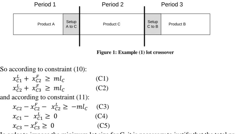
Example 1: Consider a demand for product A in period 1, for product B in period 3 and no demand in period 2. A minimum lot size is imposed on the use of shortcut product C. In this case there are two possibilities as now detailed below:
In the first possibility, setup A to C and C to B can both happen either in period two or, one setup can happen in period two and the other setup in period 1 or 3. So the minimum lot size will be enforced by constraint (11). In the second possibility, setup A to C happens in period 1 and setup C to B in period 3 while there is no setup in period 2 as shown in Figure 1.
Product A Setup Product C Product B
A to C
Setup C to B
[image:7.595.72.483.495.729.2]Period 1 Period 2 Period 3
Figure 1: Example (1) lot crossover
So according to constraint (10):
𝑥𝐶1𝐿 + 𝑥
𝐶2𝐹 ≥ 𝑚𝑙𝐶 (C1)
𝑥𝐶2𝐿 + 𝑥𝐶3𝐹 ≥ 𝑚𝑙𝐶 (C2)
and according to constraint (11):
𝑥𝐶2− 𝑥𝐶2𝐹 − 𝑥
𝐶2𝐿 ≥ −𝑚𝑙𝐶 (C3)
𝑥𝐶1− 𝑥𝐶1𝐿 ≥ 0 (C4) 𝑥𝐶3− 𝑥𝐶3𝐹 ≥ 0 (C5)
In order to impose the minimum lot size for C, it is necessary to justify that the total production of product C (at the end of period 1, in period 2 and at the beginning of period 3) is at least 𝑚𝑙𝐶:
To justify this, first constraints C1 and C2 are summed:
𝑥𝐶1𝐿 + 𝑥
𝐶2𝐹 + 𝑥𝐶2𝐿 + 𝑥𝐶3𝐹 ≥ 2𝑚𝑙𝐶 (C6)
Then constraints C3, C4 and C5 are summed:
𝑥𝐶1+ 𝑥𝐶2+ 𝑥𝐶3 ≥ 𝑥𝐶1𝐿 + 𝑥𝐶2𝐹 + 𝑥𝐶2𝐿 + 𝑥𝐶3𝐹 − 𝑚𝑙𝐶 (C7)
Finally combining constraints C6 and C7 concludes that the crossover lot of product C (𝑥𝐶1+ 𝑥𝐶2+ 𝑥𝐶3) is at least mlC and constraint (10) imposes mlC (not 2𝑚𝑙𝐶) for the whole crossover lot. Moreover this conclusion can be extended for more than one period with having no demand.
𝑥𝐶1+ 𝑥𝐶2+ 𝑥𝐶3 ≥ 𝑥𝐶1𝐿 + 𝑥𝐶2𝐹 + 𝑥𝐶2𝐿 + 𝑥𝐶3𝐹 − 𝑚𝑙𝐶 ≥ 2𝑚𝑙𝐶− 𝑚𝑙𝐶 ≥ 𝑚𝑙𝐶
Note that constraints (8) to (11) are more efficient than the conventional constraint: 𝑥𝑗𝑡 ≥
𝑚𝑙𝑗∑ 𝑦𝑖 𝑖𝑗𝑡, ∀ 𝑗, 𝑡, as used in other lot sizing and scheduling models (Clark and Clark 2000;
Fleischmann and Meyr 1997) to impose minimum lot size. The reason is that in the conventional constraint, the whole setup and the production of the minimum lot size should be carried out in a single period so the minimum lot size neither can crossover to the next period(s) nor can be produced in a period when the setup is ending at the end of previous period(s). All these restrictions are relaxed in the new constraints (8) to (11). Examples 2 and 3 in the section 2.4 show explicitly the difference of two types of constraints for imposing minimum lot size.
2.3Lot sequencing constraints
Here, the ATSP-related constraints are demonstrated for sequencing product lots. Conventional ATSP-based models restrict production to at most one lot per product per period, which may not be optimal when non-triangular setups exist. Non-triangular setups occur in industries such as food, animal feed, beverages and oil where there are intermediate “cleaning” or “shortcut” products. For example in the animal feed industry, some products can contaminate other products and lead to serious effects on animal’s health. To avoid this, machines must be cleaned, sometimes resulting in substantial setups that consume scarce production time. Alternatively, the production of a sufficient amount of an intermediate or cleaning product can clean the machines and reduce overall setup times (costs). In this situation, the setup to and from the cleaning or shortcut product (𝑘) is less costly and time consuming than a direct setup between two products (𝑖, 𝑗) means that 𝑠𝑡𝑖,𝑗 ≥ 𝑠𝑡𝑖,𝑘+ 𝑠𝑡𝑘,𝑗. Therefore the shortcut product may need to be produced more than once within a period.
1 2
13 12
3 4
15
Period t-1
S
B
C
5 6
B
8 9
7
A
16 11
10 17 18
D
Period t
Period t+1
14
A
[image:9.595.98.451.68.238.2]B
Figure 2: A main sequence (S) and different types of subtours (A, B, C, D)
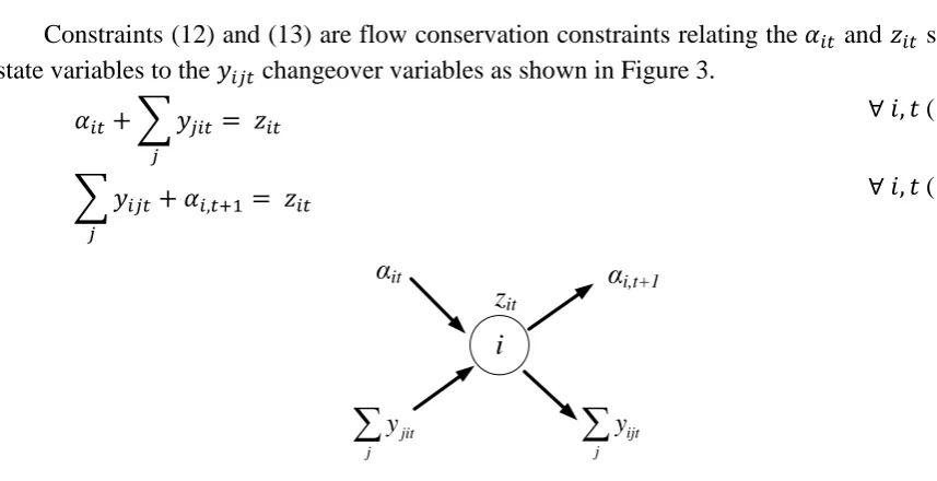
Constraints (12) and (13) are flow conservation constraints relating the 𝛼𝑖𝑡 and 𝑧𝑖𝑡 setup state variables to the 𝑦𝑖𝑗𝑡 changeover variables as shown in Figure 3.
∀ 𝑖, 𝑡 (12)
𝛼𝑖𝑡+ ∑ 𝑦𝑗𝑖𝑡
𝑗
= 𝑧𝑖𝑡
∀ 𝑖, 𝑡 (13)
∑ 𝑦𝑖𝑗𝑡
𝑗
+ 𝛼𝑖,𝑡+1 = 𝑧𝑖𝑡
αit
i
αi,t+1
zit
j ijt
y
j jit
y
Figure 1: Node flow modelled by constraints (12) and (13)
To make constraints (13) work for last period 𝑡 = 𝑇either set 𝑡 = {1, . . , 𝑇 + 1} is considered for 𝛼𝑖𝑡 or new constraints (13a) are added as follows:
∀ 𝑖, 𝑡 = 𝑇 (13a)
∑ 𝑦𝑗𝑖𝑇
𝑗
+ 𝛼𝑖,𝑇 ≥ ∑ 𝑦𝑖𝑗𝑇
𝑗
The optimal solution to the model specified so far is a sequence from product 𝑖|{𝛼𝑖𝑡 = 1} to 𝑘|{𝛼𝑘,𝑡+1 = 1} plus any disconnected subtours. The latter are excluded by imposing in every period t that there is so-called k-walk from (𝑖|{𝛼𝑖𝑡 = 1}) to all products k in the period’s sequence. From now on, 𝑝𝑡𝛼 denotes product 𝑖|{𝛼𝑖𝑡 = 1}.
Define additional binary variable 𝑎𝑖𝑗𝑡𝑘 as follows:
=1 if the arc 𝑖 → 𝑗 is on a k-walk from crossover product 𝑝𝑡𝛼 to product
k within period t’s sequence of lots, otherwise 0.
𝑎𝑖𝑗𝑡𝑘
The arc 𝑖 → 𝑗 has to exist, hence:
∀ 𝑖, 𝑗, 𝑘, 𝑡 (14)
𝑎𝑖𝑗𝑡𝑘 ≤ 𝑦
𝑖𝑗𝑡
[image:9.595.74.503.270.490.2]=1 if product i is ever in setup state in period t, otherwise 0.
𝑧𝑖𝑡𝑏𝑖𝑛
The required relationships 𝑧𝑖𝑡𝑏𝑖𝑛= 1 ⇔ 𝑧𝑖𝑡 ≥ 1 and 𝑧𝑖𝑡𝑏𝑖𝑛= 0 ⇔ 𝑧𝑖𝑡 = 0 are enforced by:
∀ 𝑖, 𝑡 (15)
𝑧𝑖𝑡 ≥ 𝑧𝑖𝑡𝑏𝑖𝑛
∀ 𝑖, 𝑡(16)
𝑧𝑖𝑡 ≤ 𝑍𝑈𝐵𝑖𝑧𝑖𝑡𝑏𝑖𝑛
Where 𝑍𝑈𝐵𝑖 is a fixed upper bound (UB) on 𝑧𝑖𝑡and greater than one. 𝑍𝑈𝐵𝑖 can be
estimated as the smaller of J (the number of products) and the size of the ordered set
{(𝑖, 𝑗)|𝑠𝑡𝑖𝑗 ≥ 𝑠𝑡𝑖𝑘+ 𝑠𝑡𝑘𝑗}, which is 1 for many non-shortcut products.
Constraints (17-19) below exclude disconnected subtours. Constraints (17) force the k -walk to reach product k and are enforced only when the setup state k exists for a time in the period (i.e, when 𝑧𝑘𝑡𝑏𝑖𝑛= 1), but not when this is never the case (when 𝑧𝑘𝑡𝑏𝑖𝑛= 0):
∀ k, t (17)
𝛼𝑘𝑡+ ∑ 𝑎𝑖𝑘𝑡𝑘
𝑖
= 𝑧𝑘𝑡𝑏𝑖𝑛
If there is no production of product k in a period, then 𝑧𝑘𝑡𝑏𝑖𝑛= 0, and by (17), 𝑎𝑖𝑘𝑡𝑘 = 0 ∀𝑖 (constraint (14) also forces this via 𝑎𝑖𝑘𝑡𝑘 ≤ 𝑦𝑖𝑘𝑡 = 0).
The k-walk corresponding to the variables {𝑎𝑖𝑗𝑡𝑘 |∀ 𝑖, 𝑗 } has to begin at 𝑝𝑡𝛼 and then pass
through other products to reach product k.
If 𝛼𝑘𝑡 = 1 then there is no need for a k-walk. If 𝛼𝑘𝑡 = 0, then by (17) ∑ 𝑎𝑖 𝑖𝑘𝑡𝑘 = 1, i.e., 𝑎𝑖𝑘𝑡𝑘 = 1 for precisely one product i, the penultimate on the k-walk. Then, by (18), 𝑎𝑗𝑖𝑡𝑘 = 1 for precisely one product j that is the 3rd last product on the k-walk, and so on, reversing along the
k-walk, requiring 𝑎𝑖𝑗𝑡𝑘 = 1 along the k-walk, finishing at the initially-setup product 𝑖 = 𝑝𝑡𝛼 (for which 𝛼𝑖𝑡 = 1).
∀ 𝑘, 𝑖 ≠ 𝑘, 𝑡(18)
𝛼𝑖𝑡+ ∑ 𝑎𝑗𝑖𝑡𝑘
𝑗
≥ ∑ 𝑎𝑖𝑗𝑡𝑘
𝑗
Constraint (19) forces the k-walk from 𝑝𝑡𝛼 to terminate at product k:
∀ 𝑘, 𝑗, 𝑡 (19)
𝑎𝑘𝑗𝑡𝑘 = 0
If there is no production of k in period t, then (19) requires 𝑎𝑘𝑗𝑡𝑘 = 0 which is not constraining as 𝑎𝑖𝑗𝑡𝑘 = 0 by (17).
The ML-SM model (Multiple Lot for Single Machine) is specified by expressions (1-19). It allows multiple production lots of shortcut products for a single machine while still not relaxing the limitations of a period’s physical separation.
2.4Period overlapping setup constraints
The last step is allowing setup operations to overlap periods, i.e., to permit a setup to begin in a period and end in the next period. The model is called MLOV-SM and relaxes all limitations of physical separation between the periods. The MLOV-SM is advantageous when capacity is tight and so lot sizing and sequencing decisions need more flexibility to reduce backlogs.
Consider the following additional decision variables:
=1 if the overlapping setup operation i to j begins in period t and finishes in period t+1, otherwise 0.
The amount of setup time that overlaps into period t+1, having begun at the end of period t.
𝑆𝑡
The value of 𝑆𝑡 must be zero if there is no overlapping last setup at the end of period t:
∀ 𝑡 (20)
𝑆𝑡 ≤ ∑ 𝑠𝑡𝑖𝑗𝑂𝐿𝑆𝑖𝑗𝑡
𝑖𝑗
The last setup and at most one setup in period t can overlap from period t to t+1:
∀ 𝑖, 𝑡 (21)
∑ 𝑂𝐿𝑆𝑗𝑖𝑡
𝑗
≤ 𝛼𝑖,𝑡+1
The value of 𝑂𝐿𝑆𝑖𝑗𝑡 must be zero if i to j is not a setup initiated in period t:
∀ 𝑖, 𝑗, 𝑡 (22)
𝑂𝐿𝑆𝑖𝑗𝑡 ≤ 𝑦𝑖𝑗𝑡
The capacity constraint (3) now becomes:
∀ 𝑡 (23)
∑ 𝑏𝑖𝑥𝑖𝑡
𝑖
+ ∑ 𝑠𝑡𝑖𝑗𝑦𝑖𝑗𝑡
𝑖𝑗
+ 𝑆𝑡−1− 𝑆𝑡+ 𝑠𝑙𝑘𝑡 = 𝐶𝑡
When the last setup is overlapping, 𝑂𝐿𝑆𝑖𝑗𝑡 = 1, then product j cannot be produced as it is
the last (crossover) lot in period t. Thus constraints (4) and (9) now become (24) and (25).
∀ 𝑗, 𝑡 (24)
𝑥𝑗𝑡 ≤ 𝑈𝐵𝑗𝑡× (𝑧𝑗𝑡− ∑ 𝑂𝐿𝑆𝑖𝑗𝑡
𝑖
)
∀ 𝑗, 𝑡 (25)
𝑥𝑗𝑡𝐿 ≤ 𝑈𝐵
𝑗𝑡 (𝛼𝑗,𝑡+1− ∑ 𝑂𝐿𝑆𝑖𝑗𝑡 𝑖
)
Thus model MLOV-SM is specified by expressions (1-2), (5-8) and (10-25) and restated completely in the Appendix A.
2.5Examples
Two examples now show the effectiveness of the new minimum lot constraints (8) to (11), in comparison with the conventional constraint (26) and also the solution’s improvement obtained by modelling setup overlapping features. The following examples are solved by three models, consisting of MLOV-SM (stated in Appendix A), ML-SM (Multiple Lot for Single Machine) which is specified by expressions (1-19), and the Conventional Model which has the same constraints as ML-SM but imposes minimum lot sizes by conventional constraint (26) rather than new imposing minimum lot sizes constraints (8) to (11).
∀ 𝑗, 𝑡 (26)
𝑥𝑗𝑡 ≥ 𝑚𝑙𝑗∑ 𝑦𝑖𝑗𝑡
𝑖
Note that in the ML-SM model, constraints (4) are valid but loose: the value of 𝑧𝑗𝑡 need
only be 1, and not ≥ 2. Thus constraints (4) can be tightened by replacing 𝑧𝑗𝑡 by 𝑧𝑗𝑡𝑏𝑖𝑛 (𝑥𝑗𝑡 ≤
𝑈𝐵𝑗𝑡× 𝑧𝑗𝑡𝑏𝑖𝑛).
Examples 2 and 3: The following data are used for both examples: 𝐶𝑡= 100, 𝑚𝑙𝑗 =
10, 𝑇 = 3, 𝐽 = 2, 𝑖0 = 1, 𝑠𝑡𝑖𝑗 = 20, 𝑏𝑗 = 1, ℎ𝑗𝑡 = 15, 𝑠𝑐𝑖𝑗 = 600, 𝑔𝑖𝑡 = 1000; and the
CPLEX 12.6 solver (CPLEX. 2014) on a computer with a 2.1 GHZ CPU and 2 GB of RAM. All models were solved in less than a second for both examples.
Table 1: Demand data for example 2 and 3.
Demand
𝑑𝒊𝒕
Example(2) Example(3)
t=1 t=2 t=3 t=1 t=2 t=3
i=1 75 0 90 75 0 90
i=2 0 90 0 0 95 0
The production diagram and the results of Example 2 are shown in Figure 4 and Table 2 respectively. Note how modelling of all necessary features of production improves the solution remarkably. As shown in Figure 4, the Conventional model cannot use the machine’s capacity efficiently and there are 5 units of idle or slack time in period 1 as the setup and minimum lot production has to be done totally in a single period (constraint (26)). This restriction is relaxed in the ML-SM model so the setup ends in period 1 and the minimum-sized lot is produced in period 2 that significantly results in a reduction of the number of inventory and backlogs as shown in Table 2. However there are still 10 units of slack time in period 2 as, in the ML-SM model, a setup cannot overlap, i.e., the setup begins in period 2 and ends in period 3. In the new lot sizing and scheduling model, MLOV-SM, all the limitations caused by previous models are relaxed and the production system is modelled realistically. Thus the scarce production capacity is used more efficiently.
Product 1 95
Product 2 80 Setup
1 to 2
Setup 2 to 1
Period 1 Period 2 Period 3
Product 1 80
Product 2 90
Product 1 80 Setup
1 to 2
Setup 2 to 1 Product 2
10 Product 170
Idle
time
Product 1 75
Product 2 90
Product 1 90 Setup
1 to 2
Setup 2 to 1
Conventional
ML-SM
MLOV-SM
Idle
time
Setup-overlapping New ml constraints
min lot
min lot
[image:12.595.114.504.387.585.2]New ml constraints
[image:12.595.71.514.652.746.2]Figure 4: Production diagram of Example 2 obtained by Conventional, ML-SM and MLOV-SM models
Table 2: Results of Example 2 obtained by Conventional, ML-SM and MLOV-SM models Example 2 Conventional ML-SM MLOV-SM
Slack capacity 5 10 0
Total Inventory 40 10 0
Backlogs 10 5 0
Total cost = Cost of
(Backlogs + Inventory +Setup)
11800 (10000+600+1200)
6350 (5000+150+1200)
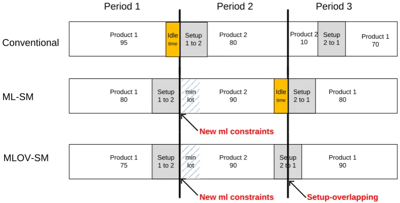
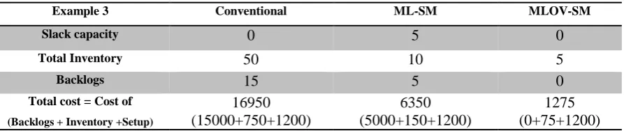
In Example 2 the optimal solution is obtained by the MLOV-SM model with no shortages or inventory. In order to tighten capacity even more, the demand of product 2 is increased to 95 in Example 3. The production diagram and the results of Example 3 are shown in Figure 5 and Table 3 respectively. Note that the Conventional model found a solution with high total inventories (50) and backlogs (15) while the optimal solution found by MLOV-SM has no backlogs and only 5 inventories.
Product 1 100
Product 2 80 Setup 1 to 2
Setup 2 to 1
Period 1 Period 2 Period 3
Product 1 80
Product 2 95
Product 1 80 Setup
1 to 2
Setup 2 to 1 Product 2
15 Product 165
Idle
time
Product 1 75
Product 2 90
Product 1 90 Setup
1 to 2
Setup 2 to 1
Conventional
ML-SM
MLOV-SM
Setup-overlapping New ml constraints
New ml constraints
P
ro
d
u
c
t2
=
5
[image:13.595.111.501.171.365.2]min lot
Figure 5: Production diagram of Example 3 obtained by Conventional, ML-SM and MLOV-SM models
[image:13.595.78.525.472.566.2]Furthermore, as shown in MLOV-SM’s production diagram in Figure 5, the minimum lot crosses over from period 1 to 2. Lot crossover is another feature which is modelled via the new minimum lot size (ml) constraints (8) to (11), improving the solutions and giving more flexibility to the lot sizing model.
Table 3: Results of Example 3 obtained by Conventional, ML-SM and MLOV-SM models
Example 3 Conventional ML-SM MLOV-SM
Slack capacity 0 5 0
Total Inventory 50 10 5
Backlogs 15 5 0
Total cost = Cost of
(Backlogs + Inventory +Setup)
16950 (15000+750+1200)
6350 (5000+150+1200)
1275 (0+75+1200)
Examples 2 and 3 showed how the new comprehensive mathematical formulation, SM, relaxes all limitations of physical separation between the periods. The MLOV-SM modelled the new features consisting of starting a setup in one period and ending it in the next period, ending a setup in a period and starting production in the next period(s), and crossing a minimum lot size over multiple periods.
3.
Computational tests
be a binary variable 𝑧𝑗𝑡 for a single machine. Thus constraints (15) and (16) disappear. The
tests also evaluated the impact of model MLOV-SM, on reducing demand backlogs, total inventory and cost in the case of tight production capacity. The models were implemented in the optimisation modelling software GAMS build 24.7.1 (Brooke et al. 1988) and solved using the CPLEX 12.6 solver (CPLEX. 2014) on a computer with a 2.1 GHZ CPU and 2 GB of RAM.
To obtain initial insights, the performance of the three models (1L-SM, ML-SM and MLOV-SM) was compared on two problem sizes: a small size with 10 products including 1 shortcut product, and a big size with 20 products including 2 shortcut products, whose lot sizes and sequences were to be scheduled over two horizons of T = 4 and T=8 demand periods.
The following data were used: 𝐶𝑡= 100, 𝑚𝑙𝑗 = 5, 𝑖0 = 1, 𝑏𝑗 = 0.5, ℎ𝑗𝑡 = 10, 𝑔𝑗𝑡 =
10000, ∀𝑗, 𝑡 for all instances. In (Clark et al. 2014) the setup times were initially set to be
𝑠𝑡𝑖𝑗 = (𝑗 − 𝑖) 𝑖𝑓 𝑗 ≥ 𝑖 otherwise (10 + 𝑗 − 𝑖), so the product 2 would normally be setup
immediately after product 1. However, product 5 was then made an extreme shortcut with zero setup times: 𝑠𝑡5𝑗 = 𝑠𝑡𝑖5 = 0. In this paper, to make setup times more tangible, particularly in
case of an overlapping setup, all setup times were increased by 3 so that 𝑠𝑡5𝑗 = 𝑠𝑡𝑖5 = 3 and
𝑠𝑡𝑖𝑗 = (3 + 𝑗 − 𝑖) 𝑖𝑓 𝑗 ≥ 𝑖 otherwise (13 + 𝑗 − 𝑖). Setup costs are proportional to setup times,
i.e.𝑠𝑐𝑖𝑗 = 50 × (𝑗 − 𝑖) 𝑖𝑓 𝑗 ≥ 𝑖, otherwise 50 × (10 + 𝑗 − 𝑖), and for shortcut products are:
𝑠𝑐5𝑗 = 𝑠𝑐𝑖5 = 50.
The periodic demand forecasts 𝑑𝑖𝑡 varied randomly over product i and period t to provoke non-uniform lot-sizes and avoid lot-for-lot production. To show the effectiveness of model MLOV-SM, the demands in two consecutive periods are set to be non-zero for different products for time horizon T=4. For example, if there are 10 products, then for period t, 5 random products have non-zero demand, with the other 5 having demand zero, while in period
t+1, those products with zero-demand in period t now have non-zero demand, with other 5 having zero demand. We also used another TBO-profile (time between orders) with different lengths 1, 2 and 3 for time horizon T=8. In this case, for each product a random TBO length (from 1 to 3) is chosen and then demands are generated for a product over 8 periods according to the TBO.
When capacity is loose, then there is much more flexibility about when setups can occur in an optimal solution, so we expect that period-overlapping setups will not make a difference. However, under tight capacity, there will be little such flexibility, so it is important to use scarce production capacity efficiently via relaxing all restrictions of physical separation between the periods. To simulate tight capacity the overall demand was adjusted so that setup times could take up to 20-25% of capacity. For loose capacity this was adjusted to 15%.
A similar procedure was applied for big size problems with 20 products. The machine capacity per period was doubled and setup times for products P11 to P20 simply replicate those for P1 to P10, with the two extreme shortcut products being P5 and P15.
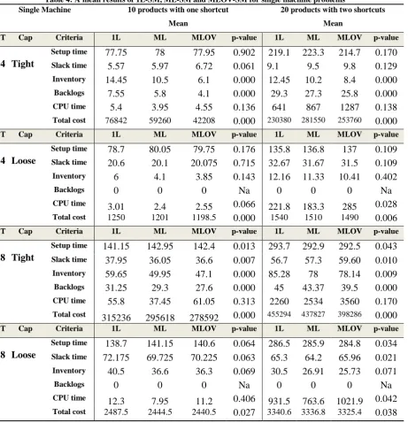
Table 4: A mean results of 1L-SM, ML-SM and MLOV-SM for single machine problems Single Machine 10 products with one shortcut
Mean
20 products with two shortcuts Mean
T Cap Criteria 1L ML MLOV p-value 1L ML MLOV p-value
4 Tight
Setup time 77.75 78 77.95 0.902 219.1 223.3 214.7 0.170 Slack time 5.57 5.97 6.72 0.061 9.1 9.5 9.8 0.129 Inventory 14.45 10.5 6.1 0.000 12.45 10.2 8.4 0.000 Backlogs 7.55 5.8 4.1 0.000 29.3 27.3 25.8 0.000 CPU time 5.4 3.95 4.55 0.136 641 867 1287 0.138 Total cost 76842 59260 42208 0.000 230380 281550 253760 0.000
T Cap Criteria 1L ML MLOV p-value 1L ML MLOV p-value
4 Loose
Setup time 78.7 80.05 79.75 0.176 135.8 136.8 137 0.109 Slack time 20.6 20.1 20.075 0.715 32.67 31.67 31.5 0.109 Inventory 6 4.1 3.85 0.143 12.16 11.33 10.41 0.402
Backlogs 0 0 0 Na 0 0 0 Na
CPU time 3.01 2.4 2.55 0.066 221.8 183.3 285 0.028 Total cost 1250 1201 1198.5 0.000 1540 1510 1490 0.006
T Cap Criteria 1L ML MLOV p-value 1L ML MLOV p-value
8 Tight
Setup time 141.15 142.95 142.4 0.013 293.7 292.9 292.5 0.043 Slack time 37.95 36.05 36.6 0.007 56.7 57.3 59.60 0.010 Inventory 59.65 49.95 47.1 0.000 85.28 78 78.14 0.009 Backlogs 31.25 29.3 27.6 0.000 45 43.37 39.5 0.000 CPU time 55.8 37.45 61.05 0.313 2260 2534 3560 0.170 Total cost 315236 295618 278592 0.000 455294 437827 398286 0.000
T Cap Criteria 1L ML MLOV p-value 1L ML MLOV p-value
8 Loose
Setup time 138.7 141.15 140.6 0.064 286.5 285.9 284.8 0.034 Slack time 72.175 69.725 70.225 0.063 65.3 64.2 65.96 0.021 Inventory 40.5 36.6 36.3 0.069 30.5 26.91 25.73 0.071
Backlogs 0 0 0 Na 0 0 0 Na
CPU time 12.3 7.95 11.2 0.406 931.5 763.6 1021.9 0.042 Total cost 2487.5 2444.5 2440.5 0.027 3340.6 3336.8 3325.4 0.038
Table 4 compare the performance of three models on 6 criteria calculated over the planning horizons 4 and 8:
Total time spent on setups = ∑ 𝑠𝑡𝑖𝑗 𝑖𝑗𝑦𝑖𝑗𝑡 Amount of unused (slack) capacity = ∑ 𝑠𝑙𝑘𝑡 𝑡 Inventory =∑ 𝐼𝑖𝑡 𝑖𝑡
Backlogs = ∑ 𝐵𝑖𝑡 𝑖𝑡 CPU time
Total cost = Backlogs + Inventory + Setup = ∑ 𝑔𝑖𝑡 𝑖𝑡𝐵𝑖𝑡+ ∑ ℎ𝑖𝑡 𝑖𝑡𝐼𝑖𝑡+ ∑ 𝑠𝑐𝑖𝑗𝑡 𝑖𝑗𝑦𝑖𝑗𝑡
For each criterion, the difference between the mean values for the three models was statistically tested using a balanced analysis of variance test. The test used the data instance (that is the run) as a random blocking factor. The null hypothesis is that the difference between the models’ means is zero.
Single Machine The paired T-test
10 products with one shortcut P-Value
20 products with two shortcuts P-Value
T Capacity Criteria 1L&ML ML&MLOV MLOV&1L 1L&ML ML&MLOV MLOV&1L
4 Tight
Setup time
0.296 0.467 0.384 0.053 0.324 0.062
Slack time 0.175 0.076 0.016 0.203 0.034 0.041 Inventory 0.005 0.049 0.003 0.006 0.038 0.001 Backlogs 0.000 0.000 0.000 0.028 0.000 0.000 CPU time 0.020 0.096 0.189 0.128 0.096 0.073 Total cost 0.000 0.000 0.000 0.000 0.000 0.000 T Capacity Criteria 1L&ML ML&MLOV MLOV&1L 1L&ML ML&MLOV MLOV&1L
4 Loose
Setup time
0.067 0.309 0.086 0.087 0.186 0.076
Slack time 0.291 0.478 0.245 0.087 0.181 0.067 Inventory 0.104 0.374 0.040 0.134 0.178 0.108
Backlogs Na Na Na Na Na Na
CPU time 0.052 0.093 0.048 0.122 0.028 0.015 Total cost 0.000 0.165 0.000 0.032 0.087 0.024 T Capacity Criteria 1L&ML ML&MLOV MLOV&1L 1L&ML ML&MLOV MLOV&1L
8 Tight
Setup time
0.011 0.009 0.046 0.008 0.006 0.012
Slack time 0.006 0.009 0.034 0.032 0.044 0.014 Inventory 0.000 0.003 0.000 0.012 0.002 0.000 Backlogs 0.001 0.000 0.000 0.002 0.000 0.000 CPU time 0.149 0.064 0.373 0.258 0.420 0.131 Total cost 0.001 0.000 0.000 0.000 0.000 0.000 T Capacity Criteria 1L&ML ML&MLOV MLOV&1L 1L&ML ML&MLOV MLOV&1L
8 Loose
Setup time
0.032 0.022 0.082 0.095 0.047 0.035
Slack time 0.033 0.032 0.078 0.033 0.016 0.024 Inventory 0.049 0.369 0.047 0.032 0.109 0.026
Backlogs Na Na Na Na Na Na
CPU time 0.135 0.034 0.393 0.183 0.045 0.023 Total cost 0.037 0.088 0.025 0.024 0.061 0.017
As expected, under loose capacity with no backlogs, due to greater flexibility in setups, period overlapping did not make a significant difference in inventory and slack time, although it significantly improved the total cost compared to the 1L model.
Not surprisingly, there were much longer solution times for 20 products than 10 products, and also for instances with T=8 periods compared to those with T=4. For 20 products and T=8 under tight capacity, 17 of the 20 instances of the MLOV model used the full 1 hour allowance of computing time (with median optimality gap of 3.7% for these 17), while none did for the 1L and ML model.
4.
Extensions to Parallel Machines and Flexible Flow Lines
In this section the Single Machine models are extended to Parallel Machines (PM) and Flexible Flow Lines (FFL). The data, variables and constraints of the Single Machine models are adapted to parallel machines by including an index m. The Multiple Lot model for Parallel Machines, denoted ML-PM, and Multiple Lot model with Setup-Overlapping for Parallel Machines, denoted MLOV-PM, are extensions of ML-SM and MLOV-SM respectively.
4.1
Parallel Machines
The input data required by the PM models are:
Demand for product i realised at the end of period t
𝑑𝑖𝑡
Available capacity time of machine m in each period t
𝐶𝑚𝑡
Time needed to setup from product i to product j on machine m
𝑠𝑡𝑖𝑗𝑚
Cost needed to setup from product i to product j on machine m
𝑠𝑐𝑖𝑗𝑚
Time needed to produce a unit of product i on machine m
𝑏𝑖𝑚
Cost of holding a unit of product i from period t to t+1
ℎ𝑖𝑡
Backlog cost per period for product i from period t to t+1
𝑔𝑖𝑡
Upper bound 𝐶𝑚𝑡⁄𝑏𝑖𝑚 on the quantity of product i produced in period t
on machine m
𝑈𝐵𝑖𝑚𝑡
The product setup at the end of period 0 on machine m, i.e., the starting setup configuration
𝑖0𝑚
The decisions variables by the PM model are represented by following variables:
Inventory level of product i at the end of period t.
𝐼𝑖𝑡
Backordered amount of product i at the end of period t.
𝐵𝑖𝑡
Production quantity of product i in period t on machine m.
𝑥𝑖𝑚𝑡
Number of unites of slack capacity of machine m in period t.
𝑆𝑙𝑘𝑚𝑡
The quantity produced in period t of the first (crossover) lot of product
i on machine m in period t if it was setup in period t-1, otherwise 0.
The quantity produced in period t of the last (crossover) lot of product i
on machine m in period t if its production continues into period t+1, otherwise 0.
𝑥𝑖𝑚𝑡𝐿
Number of times that production is to be changed over from product i to product j on machine m in period t, Integer non-negative.
𝑦𝑖𝑗𝑚𝑡
Number of times that product i is in a setup state on machine m in period
t, Integer non-negative.
𝑧𝑖𝑚𝑡
= 1 either because j-to-i is the last setup of machine m in previous periods to t or because j-to-i is the setup operation that overlaps from t-1 to
t.
𝛼𝑖𝑚𝑡
=1 if the arc 𝑖 → 𝑗 is on a walk from crossover product 𝑝𝑡𝛼 to product k
within period t’s sequence of lots on machine m, otherwise 0.
𝑎𝑖𝑗𝑚𝑡𝑘
=1 if product i is ever in setup state on machine m in period t, otherwise 0.
𝑧𝑖𝑚𝑡𝑏𝑖𝑛
=1 if the overlapping setup operation j-to-i on machine m begins in period t and finishes in period t+1.
𝑂𝐿𝑆𝑖𝑚𝑡
The amount of setup time that overlaps into period t+1 on machine m, having begun at the end of period t.
𝑆𝑚𝑡
For all the products, the initial inventory (𝐼𝑖0) and the backlogs (𝐵𝑖0) are set to be zero at
the start of the planning horizon. All the ML-PM and MLOV-PM’s constraints are similar to ML-SM and MLOV-SM respectively with the new adapted data and variables. The complete ML-PM and MLOV-PM models are presented in Appendix B and C.
Example 4: Consider 2 machines in parallel. The aim is to satisfy the demand shown in Table 6 for 10 products over the 4 planning periods with minimal backorders, inventory and setup costs. The capacity of each machine is 𝐶𝑚𝑡= 50, thus a total capacity of ∑ 𝐶𝑚 𝑚𝑡 = 100 is available for each period. The remaining PM data is the same as for the SM problem: 𝑚𝑙𝑗 =
5, 𝑖0𝑚 = 1, 𝑏𝑗𝑚 = 0.5, ℎ𝑗𝑡 = 10, 𝑔𝑗𝑡= 10000, ∀𝑗, 𝑡. Also the setup times and costs of each
machine replicate those for a single machine.
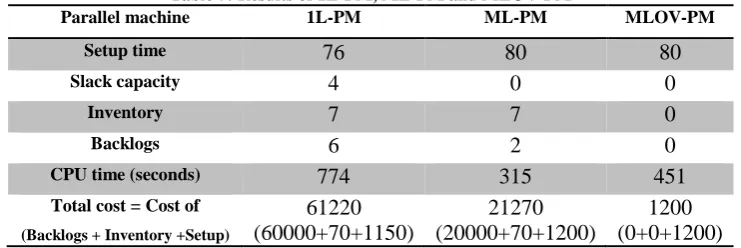
The production diagrams and the results obtained by solving the 1L-PM, ML-PM and MLOV-PM models are shown in Figure 6 and Table 7 respectively. Note that in Table 7, the 1L-PM and ML-PM model found the solution with the same amount 7 of inventory, and amounts 6 and 2 of backlogs respectively, while the optimal solution found by MLOV-PM has no backlogs or inventory.
Table 6: Demand data for PM and FFL.
𝒅𝒊𝒕 t = 1 t = 2 t = 3 t = 4
i = 1 33 0 34 0
i = 2 33 0 0 0
i = 3 31 0 33 0
i = 4 33 0 0 0
i = 6 0 33 30 33
i = 7 0 33 0 33
i = 8 0 24 32 33
i = 9 0 33 0 31
i = 10 0 31 0 33
M a c h in e 1 M a c h in e 2 1 L -P M
t = 1
10 30 9 33 8 21 8 6 5 5 3 33 1 34 8 21 7 33 6 30 10 33 9 31 8 12
t = 2 t = 3 t = 4
5 5 2 33 1 0 1 33 5 22 4 33 3 31 5 6 7 33 6 33 6 33 5 26 8 29 10 1 M a c h in e 1 M a c h in e 2
t = 1
1 24 5 25 4 33 5 5 3 31 2 33 1 11 8 12 7 33 6 33 10 31 9 33 8 10 6 33 5 29 8 26 8 8 5 5 3 33 1 32 8 21 7 33 6 30 10 33 9 31 8 12
t = 2 t = 3 t = 4
M L -P M M a c h in e 1 M a c h in e 2 M L O V -P M
t = 1
10 31 9 33 8 12 8 3 5 5 3 33 1 34 8 18 7 33 6 33 10 33 9 31 8 15
t = 2 t = 3 t = 4
[image:19.595.94.495.71.588.2]5 20 2 33 1 33 1 0 5 10 4 33 3 31 8 12 7 33 6 33 6 30 5 29 8 29
Figure 6: The production diagrams of 1L-PM, ML-PM and MLOV-PM
The solution is illustrated in Figure 6, where each node or circle shows the product at the top and its lot size at the bottom, and each arrow demonstrates a setup and an overlapped setup in bold as below:
product
Lot size
Setup Overlapped Setup
slack time. Furthermore, both the multiple lot models, ML-PM and MLOV-PM, took advantage of shortcut product 5 to reduce the backlogs, compares to the one lot model 1L-PM.
Table 7: Results of 1L-PM, ML-PM and MLOV-PM
Parallel machine 1L-PM ML-PM MLOV-PM
Setup time 76 80 80
Slack capacity 4 0 0
Inventory 7 7 0
Backlogs 6 2 0
CPU time (seconds) 774 315 451
Total cost = Cost of
(Backlogs + Inventory +Setup)
61220 (60000+70+1150)
21270 (20000+70+1200)
1200 (0+0+1200)
4.2
Flexible Flow Line
To model different machines at each stage e of an FFL, an index 𝑚𝑒 is used. There are E different stages e and 𝑀𝑒 different machines 𝑚𝑒 available for production at stage e. Apart from the inventory and backlogs variables, the FFL’s data and variables are similar to PM’s where index 𝑚 is replaced by index 𝑚𝑒. The new inventory and backlogs variables of FFL are as follows:
Inventory level of product i at stage e at the end of period t.
𝐼𝑖𝑒𝑡
Backordered amount of product i at the last stage E at the end of period t.
𝐵𝑖𝐸𝑡
Thus the new inventory balance constraints are:
∀ 𝑗, 𝑡(27)
𝐼𝑗𝐸,𝑡−1− 𝐵𝑗𝐸,𝑡−1+ ∑ 𝑥𝑗𝑚𝑒𝑡
𝑚𝐸
− 𝐼𝑗𝐸𝑡+ 𝐵𝑗𝐸𝑡= 𝑑𝑗𝑡
∀ 𝑗, 𝑡, 𝑒 = 1, … , 𝐸 − 1 (28)
𝐼𝑗𝑒,𝑡−1+ ∑ 𝑥𝑗𝑚𝑒𝑡 𝑚𝑒
− 𝐼𝑗𝑒𝑡 = ∑ 𝑥𝑗𝑚𝑒+1,𝑡+1
𝑚𝑒+1
∀ 𝑖, 𝑡(29)
𝐵𝑖𝑡𝐸 ≤ 𝐵𝑃 ∙ 𝑑𝑖𝑡
Constraints (27) and (28) express the material balance including backorders for end items and work in process respectively. Constraint (29) bounds backorders of end items in any period to be within a specified proportion of demand. This is the practiced assumptions in flexible flow shop manufacturing systems (Özdamar and Barbaroso lu 1999). Moreover the holding cost will be different at each stage so ℎ𝑖𝑡 now becomes ℎ𝑖𝑒𝑡 which is the cost of holding a unit of product i from period t to t+1 at stage e. The complete models for Multiple Lots for Flexible Flow Lines, denoted ML-FFL, and Multiple Lots with Setup-Overlapping for Flexible Flow Lines, denoted MLOV-FFL, are presented in Appendices D and E respectively. Apart from the inventory balance constraints, the FFL’s constraints are similar to PM’s substituting index 𝑚
with index 𝑚𝑒.
product i is 10 and for the subsequent stages, hite = VAP ∙ hit,e-1, 𝑒 ≥ 2. Thus the second
stage’s unit holding cost ℎ𝑖𝑡2 for product i is ℎ𝑖𝑡2 = 1.2 × 10 = 12.
To analyse the FFL in detail, it was solved by the three models 1L-FFL, ML- FFL and MLOV- FFL considering the demand of first and second period in Table 6. The production diagrams and the results of FFL for two periods are shown in Figure 7 and Table 8 respectively.
In order to simplify the FFL production diagram, the one-period-backward shifted demand is considered for intermediate stages (𝑒 < 𝐸), meaning that 𝑥𝑗𝑚𝑒+1,𝑡+1 in the right hand of
equation (28) changes to 𝑥𝑗𝑚𝑒+1𝑡. Thus for first stage, the inventory balance equation would be
𝐼𝑗1,𝑡−1+ ∑𝑚1𝑥𝑗𝑚1𝑡− 𝐼𝑗1𝑡 = ∑𝑚2𝑥𝑗𝑚2𝑡, ∀𝑗, 𝑡.
Table 8: Results of 1L-FFL, ML-FFL and MLOV-FFL for FFL problem with two periods Flexible Flow Line 1L-FFL ML-FFL MLOV-FFL
Setup time 78 86 86
Slack capacity 9 2 0
Inventory 3 0 0
Backlogs 6 2 0
CPU time (seconds) 623 662 656 Total cost = Cost of
(Backlogs + Inventory +Setup)
61236 (60000+36+1200)
21300 (20000+0+1300)
1300 (0+0+1300)
5 12
2 33
t = 1 t = 2
1 0 5 16 4 33 9 33 8 20 10 31 S ta g e 1 M a c h in e 1 M a c h in e 1 M a c h in e 2 7 33 6 33 5 5 9 33 8 20 10 31 1 33 1L-FFL 3 31 5 23 2 33 1 22 7 33 6 33 5 5 1 11 5 5 4 33 3 31 1 0 5 10 4 33 3 31
t = 1 t = 2
1 33 5 20 2 33 5 5 3 31 2 33 1 11 1 22 5 25 4 33 9 33 8 10 10 31 7 33 6 31 8 14 S ta g e 1 S ta g e 2 M a c h in e 1 M a c h in e 1 M a c h in e 2 M a c h in e 2 7 33 6 31 8 14 9 33 8 10 10 31 ML-FFL
t = 1 t = 2
5 14 3 31 2 33 1 0 1 33 5 16 4 33 9 33 8 10 10 31 7 33 6 33 8 14 S ta g e 1 M a c h in e 1 M a c h in e 1 M a c h in e 2 M a c h in e 2 7 33 6 33 8 12 9 33 8 12 10 31 5 16 3 31 2 33 1 0 1 33 5 14 4 33 MLOV-FFL S ta g e 2 S ta g e 2 M a c h in e 2
4.3
Computational tests
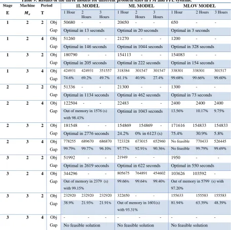
[image:23.595.87.544.165.620.2]To obtain some insight into the relative efficiencies of the three models in PM and FFL, a variety of problem sizes are solved in a three-hour time limit considering demand over 2 and 4 periods, similar to Table 6. The objective function and the CPLEX optimality gap of the models after every hour are shown in Table 9 for each problem size.
Table 9: Results of the three models for different problem sizes in PM and FFL systems.
Stage
E
Machine
𝑴𝒆
Period
T
1L MODEL ML MODEL MLOV MODEL
1 Hour 2 Hours
3 Hours
1 Hour 2 Hours
3 Hours
1 Hour 2 Hours 3 Hours
1 2 2 Obj Gap
50680 - - 20650 - - 650 - -
Optimal in 13 seconds Optimal in 20 seconds Optimal in 3 seconds
1 2 4 Obj Gap
51260 - - 21270 - - 1200 - -
Optimal in 146 seconds Optimal in 1044 seconds Optimal in 328 seconds
1 3 2 Obj Gap
180790 - - 154113 - - 154083 - -
Optimal in 205 seconds Optimal in 222 seconds Optimal in 154 seconds
1 3 4 Obj Gap
424931 424931 351557 318384 301547 301547 338301 338301 301517 74.6% 69.2% 49.7% 61.1% 40.9% 27.4% 99.68% 99.66% 99.60%
2 2 2 Obj Gap
51336 - - 21300 - - 1300 - -
Optimal in 1134 seconds Optimal in 462 seconds Optimal in 73 seconds
2 2 4 Obj Gap
122504 - - 22483 - - 2400 2400 2400
Out of memory in 1576 (s) with 98.43%
Optimal in 1043 seconds 13.56% 10.17% 9.75%
2 3 2 Obj Gap
181548 - - 154869 154869 - 171616 154833 154833
Optimal in 2776 seconds 24.2% 0% in 6123 (s) 75.4% 30.9% 5.8%
2 3 4 Obj Gap
778255 689670 686870 723328 673015 652960 No feasible 770433 526445 99.79% 99.77% 96.10% 97.77% 92.91% 90.36% No feasible 99.79% 99.69%
3 2 2 Obj Gap
51992 - - 21949 - - 1950 - -
Optimal in 2619 seconds Optimal in 622 seconds Optimal in 550 seconds
3 2 4 Obj Gap
344296 - - 805675 764891 454602 103626 103592 -
Out of memory in 2379 (s) with 99.15%
99.66% 99.64% 99.40% Out of memory in 5799 (s) with 97.20%
3 3 2 Obj Gap
232920 232920 232920 322650 - - 155633 155583 155583 38.9% 21.93% 21.91% Out of memory in 1601(s)
with 93.31%
81.94% 63.39% 48.39%
3 3 4 Obj Gap
- - - -
No feasible solution No feasible solution No feasible solution
The test results in Table 9 show, for all problem sizes, that the MLOV model obtains a better solution than the ML and 1L models after three hours and that ML is more efficient than 1L due to its use of the shortcut product. However in large instances, the models left large optimality gaps, particularly MLOV due to its extra binary variables
𝑂𝐿𝑆𝑖𝑗𝑚𝑒𝑡 for overlapping setups.
time limit, emphasizing the need for an efficient heuristic solution procedure for large problems.
5.
Final remarks
This paper presented new mix integer programming formulations for capacitated lot sizing and scheduling with non-triangular sequence-dependent setup times and costs, incorporating all the necessary features of setup carryover and overlapping on different machine configurations. These features relax all limitations of physical separation between the periods provide more flexibility to the lot sizing model.
To assess how effectively the multiple lot model with setup overlapping took advantage of shortcut products and setup overlapping features to reduce backlogs and inventory, three models 1L, ML and MLOV were compared for three production systems SM, PM and FFL. The computational results showed that the multiple-lots and setup overlapping features of the model enable more efficient production than when the formulation excludes setup overlapping or is restricted to single lot per product per product.
On a single machine the results showed highly significant decreases in backlogs, inventory and total costs for the MLOV-SM model compared to those for the ML-SM and 1L-SM models. Furthermore ML-1L-SM is more efficient than 1L-1L-SM due to its use of the shortcut product 5 to economise on setups and reduce backlogs and inventory.
The tests on the PM and FFL models also confirmed the effectiveness of the new formulation. However, because of the increased number of binary variables in large instances, CPLEX exhausted the available RAM before terminating the branch-&-cut search and leaving a large optimality gap.
To sum up, the test results above, although merely probing, and not conclusive, indicate that for all machine configurations the MLOV model obtains a better solution. Due to the importance of the number of binary variables in large instances, future research needs to develop efficient solution methods fordifferent machine configurations. Future work will also computationally compare different demand data patterns with variables sizes on the SM, PM and FFL models.
The High Multiplicity Travelling Salesman Problem (HMATSP) is a special type of the classical travelling salesman problem in which each node is visited multiple times. Sarin et al. (2011) incorporated the HMATSP model as a substructure to formulate lot-sizing problem involving parallel machines and sequence-dependent setup costs, also known as the Chesapeake Problem. The HMATSP can also be applied for scheduling family products with several identical items to be produced separately on a single machine. Modelling Multiple-Lot production per period based on the HMATSP formulations poses a very interesting challenge for future research.
While the multi-commodity flow (MCF) subtour elimination constraints do provide much tighter formulations, it is recognised that their inclusion can be increase computational time in larger-sized models. The challenge of improving computing times is left for future research.
to whether the quantity of cleaning product called minimum lot size is sequence dependent. This poses another research challenge about how to model the sequence-dependency of minimum lot sizes in lot sizing and scheduling problems.
References
Almada-lobo B, Klabjan D, carravilla MA, Oliveira J (2007) Single machine multi-product capacitated lot sizing with sequence-dependent setups International Journal of Production Research 45:4873-4894
Belo-Filho MrAF, Toledo FMB, Almada-Lobo B (2013) Models for capacitated lot-sizing problem with backlogging, setup carryover and crossover Journal of the Operational Research Society 65:1735-1747
Bitran GR, Yanasse HH (1982) Computational complexity of the capacitated lot size problem Management Science 28:1174-1186
Brooke A, Kendrick D, Meeraus A (1988) GAMS. General Algebraic Modeling System, A user guide. The Scientific Press, South San Francisco, CA
Clark A, Mahdieh M, Rangel S (2014) Production lot sizing and scheduling with non-triangular sequence-dependent setup times International Journal of Production Research 52:8:2490-2503
Clark AR, Clark SJ (2000) Rolling-horizon lot-sizing when set-up times are sequence-dependent International Journal of Production Research 38:2287-2307
Clark AR, Morabito R, Toso EAV (2010) Production setup-sequencing and lot-sizing at an animal nutrition plant through ATSP subtour elimination and patching Journal of Scheduling 13:111-121
Claus A (1984) A new formulation for the travelling salesman problem SIAM journal on algebraic and discrete methods 5:21
Copil K, Worbelauer M, Meyr H, Tempelmeier H (2016) Simultaneous lotsizing and scheduling problems: a classification and review of models Or Spectrum:1-64
CPLEX. (2014) Software package, CPLEX. 12.6. New York, USA
Desrochers M, Laporte G (1991) Improvements and extensions to the Miller-Tucker-Zemlin subtour elimination constraints Operations Research Letters 10:27-36
Eppen GD, Martin RK (1987) Solving multi-item capacitated lot-sizing problems using variable redefinition Operations Research:832-848
Fleischmann B (1990) The discrete lot-sizing and scheduling problem European Journal of Operational Research 44:337-348
Fleischmann B, Meyr H (1997) The general lotsizing and scheduling problem OR Spectrum 19:11-21 Gopalakrishnan M (2000) A modified framework for modelling set-up carryover in the capacitated
lotsizing problem International Journal of Production Research 38:3421-3424
Gopalakrishnan M, Ding K, Bourjolly JM, Mohan S (2001) A tabu-search heuristic for the capacitated lot-sizing problem with set-up carryover Management Science:851-863
Gopalakrishnan M, Miller DM, Schmidt CP (1995) A framework for modelling setup carryover in the capacitated lot sizing problem International Journal of Production Research 33:1973-1988 Günther H-O (2014) The block planning approach for continuous time-based dynamic lot sizing and
scheduling Business Research 7:51-76
Günther HO, Grunow M, Neuhaus U (2006) Realizing block planning concepts in make-and-pack production using MILP modelling and SAP APOآ© International Journal of Production Research 44:3711-3726