error-related potentials and their consequences for
classification
Mohammad Abu-Alqumsan1, Christoph Kapeller2,3,
Christoph Hinterm¨uller2,3, Christoph Guger2,3 and
Angelika Peer4
1 Chair of Automatic Control Engineering, Technical University of Munich
(TUM), Munich, Germany
2 Guger Technologies OG, Graz, Austria
3 g.tec medical engineering GmbH, Schiedlberg, Austria
4 Bristol Robotics Laboratory, University of the West of England, Bristol, UK
E-mail: [email protected]
Abstract.
Objective. This paper discusses the invariance and variability in interaction error-related potentials (ErrPs), where a special focus is laid upon the factors of (1) the human mental processing required to assess interface actions (2) time (3) subjects. Approach. Three different experiments were designed as to vary primarily with respect to the mental processes that are necessary to assess whether an interface error has occurred or not. The three experiments were carried out with 11 subjects in a repeated-measures experimental design. To study the effect of time, a subset of the recruited subjects additionally performed the same experiments on different days. Main results. The ErrP variability across the different experiments for the same subjects was found largely attributable to the different mental processing required to assess interface actions. Nonetheless, we found that interaction ErrPs are empirically invariant over time (for the same subject and same interface) and to a lesser extent across subjects (for the same interface). Significance. The obtained results may be used to explain across-study variability of ErrPs, as well as to define guidelines for approaches to the ErrP classifier transferability problem.
Keywords: EEG, BCI, Error-related Potentials, P300, invariance, classification
1. Introduction
Error processing and awareness mechanisms in the brain lead to reproducible brain activity patterns, which can be observed in scalp EEG time-locked to events of errors. In general, these patterns are referred to as error-related potentials (ErrPs) and are typically taxonomized into four types: response, observation, feedback and interaction ErrPs [1, 2]. This taxonomy basically reflects the variability in the error potentials with respect to changes in the tasks, in which they have been observed. Response ErrPs were found to be elicited after incorrect responses in speeded choice reaction time (RT) tasks [3,4]. ObservationErrPs, on the other hand, have been shown to be elicited after observing errors committed by other humans [5] or virtual devices [6,7] in different tasks including speeded choice RT. Feedback ErrPs are elicited after negative feedback (e.g. feedback of unfavorable results in time estimation tasks) [8–10]. Finally, interaction ErrPs were reported after feedback that indicates erroneous interface actions [11, 12], and therefore they can be thought of as a special case ofobservation andfeedback ErrPs.
The average difference waveform in the event-related potential (ERP) structure between the error and correct trials (error-minus-correct) is usually used to highlight the ErrP components. For instance, the difference waveform of response ErrPs has been characterized by Falkenstein et al. [3] with a negativity Ne (sometimes referred to as error-related negativity ERN) and a later, more extended positivity Pe. The sharp negative component, Ne, peaked at about 80 ms and was maximal at midline frontocentral scalp locations, whereas the positivity, Pe, peaked in the interval 200-500 ms after incorrect key presses [13]. The Pe was shown in a more recent study to have two subcomponents, with frontocentral and centroparietal distributions [14]. The negativity was also observed in correct trials, however with smaller amplitudes (referred to as correct-related negativity CRN). According to [13], the presence of CRN might indicate that the negativity Ne reflects the comparison process itself (between the correct and performed response) and not its outcome, and that the independent component Pe reflects a later aspect of the error processing, e.g. error awareness [14, 15].
In addition to the temporal (phase-locked) signature of errors in scalp EEG, spectral (phase- and
non-phase-locked) signatures were observed starting just before incorrect presses in speeded motor responses manifested as an increase in mid-frontal theta band activity accounting for 57% of ERN peak amplitude [16], and an increase in delta-power [4]. The respective temporal and/or spectral signatures may vary across the different types of ErrPs; nonetheless, independent of the specific type of error potentials and independent of the task performed, EEG and fMRI studies in humans [8, 13, 17–19] and single-unit studies in monkeys [20, 21] have suggested the anterior cingulate cortex (ACC), the supplementary motor Area (SMA), and/or pre-SMA (all in the posterior medial frontal cortex, pMFC) as candidates for a common neural generator. This in turn suggests that the different ErrP types are manifestations of similar performance monitoring systems [22–25]. Furthermore, errors, and more specifically, conscious errors, are accompanied by changes in autonomic activity, like heart rate deceleration, increase in pupil size, larger skin conductance responses and increased amygdala activity [15].
Schalk et al. [11] were the first to report that EEG signals that follow erroneous and correct selections by a computer interface differ significantly. The term interaction ErrPs has been coined later by Ferrez et al. [12] to refer to this type of ErrPs. Thereafter, there has been a special interest in interaction ErrPs within the field of brain-computer interfaces (BCIs), that concerns itself with providing users, particularly those living with disabilities, with control and communication abilities on the basis of their measurable brain neural activity. Hereby, the presence or absence ofinteraction ErrPs in scalp EEG can be used as a means to respectively invalidate or validate a first-stage BCI selection. The first selection can be mediated based on P300, SSVEP or motor-imagery (MI) signals, whose classification is known to be prone to errors due to the inherent presence of noise in scalp EEG. The amplitude of the noise (background activity in the brain and bodily artifacts) can be of several orders of magnitude above the amplitude of ERPs [26, 27].
rate in addition to the accuracy improvement. It can be shown, nonetheless, that if the interface parameters remain the same (i.e. with respect to the number of interface elements, time for a single selection, interaction paradigm, etc.) for both the selection and verification steps, a significant loss in achievable bit rates is then expected for almost all levels of single trial accuracies (see the supplementary material for more details). On the other hand, integrating the detection of ErrPs into different practical BCI systems [11,12,29–33] improved both the accuracy and the achieved bit rates. High false alarm (i.e. estimating trials as erroneous when they are not) rates, however, may degrade the achieved bit rate and interaction speed [32].
Typically, training sessions that contain a consi-derable amount of ErrP/noErrP examples are used to learn classification boundaries that separate the two classes. For the different types of BCIs, including those based on ErrPs, it is generally desirable to reuse previ-ously recorded sessions in training classifiers that can be used across different tasks, on different days, or/and with different subjects [34]. This is, however, made difficult, with the considerable (between and within-subjects) fluctuations in the underlying statistics of the brain patterns under consideration [35, 36]. Fluc-tuations, due to the non-stationarity dynamics of the brain, may result in trial-to-trial variability [37] and latency jitter of the ERP components on session-to-session basis [38] and may lead to reduced accuracy levels when going from the calibration (i.e. training) phase of classifiers to their online usage, even with the same subjects, on the same days and with the same interfaces/tasks [36, 39].
However, and apart from the EEG non-stationarity, there exist invariant features that make ErrPs visible and reproducible in the first place. In the present work, it is investigated whether there are invariants of interaction ErrPs and the consequences these invariants, if any, might have for their classifica-tion. Our main focus was to check possible invariants with respect to: (1) human mental processes that are required after feedback onset (2) time (3) subjects.
The variability in interaction ErrPs across the different levels of a certain experimental factor is expressed hereby in terms of the observed differences in the temporal evolution and morphology of the average ErrP waveforms. The notion of invariance, on the other hand, is used throughout this work as underlying this very notion of variability. Hereby, the association between the two terms is similar to that in studies of speech processes (e.g. [40]), where despite the existing between and within-talker variability with respect to speech signals (e.g. vocal pitch, volume, fluency), there are invariant features that allow their listeners
to recognize the intended meaning. By analogy, it is reasoned here that should there exist some statistically invariant features of interaction ErrPs across the different levels of a certain experimental factor, then data obtained at a certain level can be used reliably to draw a linear plane separating error and correct trials obtained at different level(s). Invariance with respect to a specific factor is hereby measured with the accuracy of classifier transfer across the different levels of this factor. Classification accuracies are quantified by the normalized mutual information (NMI), which is used to summarize the classification sensitivity and specificity with a single metric [2].
In order to answer the questions raised above, three different experiments and tasks were designed and conducted with different subjects. The first ex-periment is quite similar to the keyboard-based cursor movement in [12] and the other two experiments, simi-lar to [30], were based on P300-mediated interaction. Some closely related work to ours exists in [41] for ob-servation ErrPs and [42] for different types of errors. The main result of this work is that we show that in-teraction ErrPs (1) are highly sensitive with respect to the mental processing required to assess interface acti-ons (2) are quite empirically invariant over time for the same interface (3) have invariant features across subjects for the same interface. It is also observed that ErrPs are sensitive to the details of the EEG pre-processing pipeline. This may explain the ErrP vari-ability across studies of similar nature regarding the mental processes of the interface actions.
Prior research on ErrPs have partially tackled some of these issues at separate occasions (see Section 2), which helped to formulate first hypot-heses and guided the design of the three interfa-ces/experiments. With this work, the aim is to ground irrelevant factors in the experimental design and in the pre-processing pipeline so that concrete conclusi-ons can be drawn with respect to the different sources of invariance and variability under consideration. To the best of our knowledge, this is the first work that tackles such sources from a unified perspective.
This paper is structured as follows. Section 2 provides a short review on related work and similar experiments to ours. Section 3 reports the materials and the design of the different experiments conducted in this work. Experimental results are presented in section 4 followed by a discussion in section 5. This paper concludes with section 6.
2. Related work
Across these studies, one can observe that many aspects remained invariant whereas many others have shown great variability. The current work builds on findings from these studies and tries to extend our understanding of the sources of variability and invariance ininteraction ErrPs.
2.1. Invariance with respect to human mental processes consequent to the feedback onset
In one-dimensional cursor control using MI-based BCI (based on modulation of µ and β rhythms) [11], it has been shown that the difference waveform (error-minus-correct) is characterized by a positive potential centered at the vertex peaking around 180 ms. Despite that the cursor was required to be moved incrementally towards the goal, the error and correct trials were defined solely based on the correctness of the final destination. In quite similar experiments [12], the MI-based interface was simulated by keyboard presses and each intermediate step towards the goal was labeled either as a correct or erroneous trial. The difference waveform time-locked to cursor movements (i.e. feedback onset) was shown to have a sharp negative peak after 250 ms (N2) followed by a positive peak after 320 ms (P3) and a second broader negative peak after 450 ms (N4). These peaks clearly differ from the positive potential in [11], and this discrepancy can be attributed to the different mental processes required to evaluate whether or not a cursor arrives at the target goal and whether or not it just moves towards it [29].
Similarly, in experiments where subjects observed and evaluated the movements of a virtual device towards cued goals, Iturrate et al. [41] have shown that slight changes in the performed tasks lead to significant differences in the peak latency of N2, P3 and P4 in observation ErrPs. The tasks differed only in the way the virtual device moved with respect to the cued goals (either with incremental steps in a horizontal and vertical grids or with a single jump). The observed signal variations were shown additionally, to make it difficult for a classifier trained with data from one task to straightforwardly transfer to other ones. Yet, recalibration and adaptation of the learned classifier (by adapting the means of correct and incorrect trials to the new task) provided fairly good results when a few training examples for the new task were available [41]. Further, using three different experimental protocols in [43], where users evaluated the movements of a virtual square, a simulated robotic arm and a real robot arm, differences in peak latencies of P3 and N4 in observation ErrPs across these experiments were reported to be significant, whereas differences in peak amplitudes were not. As the average waveforms of correct and error trials were observed to be similar with respect to the general shape
across experiments, correcting single trial data for the observed latency differences was shown to enhance classifier generalizability across tasks.
Furthermore, in a simple video game task with continuous feedback, where users used a gamepad to control a cursor to avoid collisions with blocks dropping from the top of the screen with constant speeds, different kinds of errors were found to produce different and distinguishable ErrP waveforms with different spectral contents [2, 42]. The examined errors were either due to inaccurate feedback (i.e. cursor moved deliberately in directions that differ from the user input) or due to failing to achieve target goals (i.e. user input led to collisions with the moving objects). The two errors were respectively referred to by the authors asexecution andoutcome errors. Our thinking is that such differences in the morphology of the difference waveforms across the two types of errors stem from the different mental processes required to assess the feedback stimuli. In particular, the shape and the scalp topography of execution errors are reported to have N2, P3 and N4 components, similar to those reported in interaction ErrPs [12] and observation ErrPs [41], where judging the correctness of interface actions is achieved by mentally evaluating whether a cursor moved as signaled/expected or not.
On a different vein, some variability in the ErrP waveforms can be observed across hybrid P300-ErrP systems, where different feedback presentation methods have been deployed. For instance, authors in [29, 44, 45] adopted a central feedback presentation, whereby the selected character was shown overlaid at the center of the spelling matrix, 1 second or more after the row-column flashing is stopped. The central feedback strategy was also employed in a modified way in [30], where the character presentation is preceded by a presentation of an empty square at the center of the display aiming at attracting the user visual attention to that spot before the estimated character is presented at the same location on the display. This way, ocular artifacts can be reduced. The observed grand average difference waveform at Cz for a group of healthy subjects was characterized by a negativity at around 348 ms and a later positivity at around 465 ms [30]. Alternatively, the feedback in [46] was done by replacing all the matrix elements with the estimated one.
signals vary as a byproduct. For instance, the central feedback, when used in language spelling tasks, requires that the users remember (though for a very short time) the last character, to which they attended, and compare it with the estimated one. Users may not need to perform this comparison (or even memorization) when the replacement feedback in [46] is used, since in this case a visual change of the character at the attended place in the P300 matrix simply means that the interface made an error. Consequently, one can observe a great discrepancy in the two ErrP waveforms in [30] and [46] (polarities of the different peaks in the two signals appear to be reversed).
2.2. Invariance with respect to user input
In an attempt to reduce the time required to collect ErrP/noErrP training data, Schmidt et al. [32] have designed a calibration keyboard-based experiment for the P300 center speller [47], in which the post-feedback behavior of the interface is identical to that in the P300 case. This way, authors make sure that the mental processes required to assess the feedback as correct/erroneous are identical across the keyboard-calibration and P300-online conditions. Herein, visual inspection of the grand averages of the erroneous and correct trials reveals a great similarity across the two tasks with respect to the general shape. However, the error negativity (Ne) and positivity (Pe) of the difference waveform were observed with stronger amplitudes and earlier in time in the online condition compared to calibration. A linear discriminant analysis (LDA) classifier for interaction ErrPs trained with data from the calibration experiments was shown to transfer, however with a reduced performance, to the P300-based online sessions.
Furthermore, Kim and Kirchner [7] designed a task to compareobservationErrPs (users observed the movement of a cursor with no input whatsoever) and interaction ErrPs (users controlled the movement of a cursor with a noisy keyboard). Hereby, interaction ErrPs appeared after cursor movements in directions that do not match the user’s keyboard presses, while observation ErrPs appeared when an observed agent moved in directions that deviate from a hard-coded path. It was observed that the grand average difference waveforms of the two ErrP types have similar shapes in the early time region 0.16-0.4 s, but exhibit different shapes in the late time region 0.4-0.8 s. Arguably, this discrepancy might be attributed to the overlap of errenous and correct trials as a result of the used experimental paradigms, and/or the fact that the two tasks differed in that key presses were self-paced in the interaction task and hard-coded within predefined intervals in case of the observed agent. The authors
have shown that a linear support vector machine (SVM) classifier learned from the observation ErrPs can successfully transfer to interaction ErrPs. The classifier transfer in the reverse direction (i.e. from interaction to observation) was also successful but with a reduced performance.
Taking advantage of these results, it may be assumed that if two tasks differed with respect to the type of the user input, and a sufficient time gap was introduced between the arrival time of the user input and the onset time of the feedback stimulus, then any observed variability in the ErrP waveforms consequent to the feedback onset across the two tasks is most likely caused by other factors than the discrepancy in user input.
2.3. Invariance with respect to time
Ferrez et al. [12] have shown interaction ErrPs to be stable over time as the average difference waveforms and scalp topographies remained similar for two recordings spaced about three months apart. Additionally, a Gaussian classifier trained with data from the first recording was reported to produce relatively high accuracy levels (about 80%) when applied on the data from the second recording.
2.4. Invariance with respect to subjects
It is argued in [48] that ERN is a subjective response that is influenced by individual differences in cognitive modeling of what is being correct/incorrect. This is supported by evidences from different studies which show e.g. that the magnitude of ERN is correlated with the level of academic performance of subjects [24] and that the level of ACC and pre-SMA activation and magnitude of ERN is correlated with age [49, 50].
However, despite this inter-subject variability, no significant difference in peak latency or peak-to-peak amplitude of interaction ErrPs has been observed across the groups of healthy and motor-impaired subjects [30]. Further, it has been shown in [7, 51] that a classifier learned from examples of interaction ErrPs obtained from the EEG of several subjects time-locked to erroneous/correct interactions can transfer to new subjects performing the same task with relatively good accuracy (75% on average). The across-subjects classifier transfer, for most subjects, performed worse than a classifier transfer among different types (observation to interaction and vice versa) of ErrPs within the same subjects [7].
3. Material and methods
subjects and over time, which was also confirmed with the possible classifier transfer across these factors. In this work, we argue that the discrepancy in the mental processes required to assess interface actions accounts for much of the variability observed across different studies. This hypothesis is tested in the present work using a repeated-measures experimental design, where the same subjects performed three experiments on different days. The tasks in two experiments are designed to be exactly the same, except for the way the visual feedback is provided to users. Additionally, to ground the effect of time, a small sample of the recruited participants performed the same experiments, for multiple times on different days.
3.1. Subjects
A total of 11 healthy adults (7 male, 4 female) aged 27.4±5.7 (range 19−39) served as paid volunteer subjects in this study. S10 was left-handed and all subjects except S2 had normal or corrected-to-normal vision. Subject S2 had extreme hyperopia in the left eye. All subjects were na¨ıve as to the purposes of the experiments. Subject S11 was excluded from the study for not being able to use the P300 speller.
3.2. Data recording
During the different experiments, the participants were seated 0.7 m away from an LCD monitor on a comfortable armchair in a slightly dimmed room. All participants gave their written informed consent. Participants were additionally asked to fill in pre-and post-questionnaires, that were meant to collect data about the level of tiredness before and after the experiment in addition to some demographical data. This data, however, was not used for the purposes of this study.
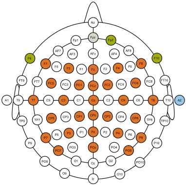
Scalp EEG signals were recorded from 28 electrodes positioned according to the international extended 10/20 electrode system at F7, F3, Fz, F4, F8, FC5, FC1, FCz, FC2, FC6, T7, C3, Cz, C4, T8, CP5, CP1, CPz, CP2, CP6, P7, P3, Pz, P4, P8, PO7, POz and PO8 as shown in figure 1. Similar to [52, 53], Electrooculogram (EOG) traces were obtained from electrodes F9, F10, FP2 and an additional electrode placed directly below the right eye. EEG and EOG electrodes were referenced to the right earlobe and the ground electrode was positioned at FPz. The horizontal bipolar EOG (HEOG) signal was computed from the raw data of electrodes F9 and F10. Similarily, vertical bipolar EOG (VEOG) was computed from FP2 and the electrode placed below the right eye.
EEG and EOG data were measured with sampling rate of 256 Hz at full DC using g.USBamp
Nz
CPz Fpz
AFz
Fz
FCz
Cz
Pz
POz
Oz
Iz
Fp1 Fp2
AF3 AF4
AF7 AF8
F7
F5 F3 F1 F2 F4 F6 F8 F9
FT9 FT7 FC5 FC3 FC1 FC2 FC4 FC6 FC8 F10
FT10
A1 T9 T7 C5 C3 C1 C2 C4 C6 T8 T10 A2
TP10
P10 TP8
P8
PO8
O2 PO4 P2 P4 P6 CP2 CP4 CP6 TP9 TP7 CP5 CP3 CP1
P9 P7 P5
P3 P1
PO7 PO3
O1 PO9
O9
PO10
[image:6.612.333.524.62.252.2]O10
Figure 1: EEG/EOG electrode placement.
acquisition system (g.tec medical engineering GmbH, Schiedlberg, Austria). All electrodes were filled with highly conductive gel in order to reduce impedance. Participants were free to move their eyes during the recordings, but were instructed to reduce all unnecessary muscular activity.
3.3. Experimental paradigms
g.USBamp Acquisition System
Recording & Processing Computer
Stimuli Visualization
[image:7.612.316.551.62.173.2]Computer
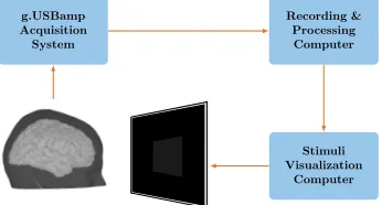
Figure 2: System overview showing the main modules. Recording and stimulation were done on the same machine for Exp. I. Visual stimuli were presented on a 60 Hz LCD monitor.
sessions and trials varied across subjects.
In all experiments, participants were instructed to mentally evaluate the interface actions as correct or erroneous. Figure 2 shows the main modules used for the experimental setup in all three experiments, where the acquisition of the data and offline processing were facilitated with Simulink/MATLAB software (MathWorks, Massachusetts, United States). The experimental design for each of the experiments is described in the following subsections, and a summary that relates the respective tasks and explains the reasons behind their choice will be presented in subsection 3.3.4.
3.3.1. Experiment I: Keyboard-mediated ball game task Very similar to [12], participants were instructed to use the left and the right arrow keyboard keys in order to move a ball towards a hole (respectively the sphere and the rectangle in figure 3), where both were aligned to the same horizontal line at the middle of the display. Each game run started with the ball randomly placed 5 steps away from the hole, either to the right or to the left with equal probabilities. In this work, we refer to all trials that are recorded while the hole is being to the right of the ball as right trials and otherwise as left trials. Following each key press issued by the participant, the ball moved one step in the direction of the pressed key with a probability of 80% and in the opposite direction with the remaining probability. In order to isolate motor-related potentials due to key presses from potentials following the feedback presentation, the ball appeared in the new location
τ s after each key press, where τ is uniformly drawn in the interval [0.9,1.1] s. Immediately after key presses, the color of the ball turned from green into red, indicating that further key presses will be ignored and the ball remained red for a period of 2 s. Subjects were instructed not to try to interact with the ball during this time. Once the ball reached the hole, a new game run was started after 2 s. Each subject finished
t t1
t2
t3
t4
Figure 3: Key events in the keyboard-based interaction experiment. At timet1, the user presses the key which brings the ball towards the hole (left key in the shown case). In the next display frame, the ball turns red and stays in place for a duration randomly drawn from the interval [0.9,1.1] s. Afterwards at t3, the ball moves one step either to the right or the left according to user input and the error random generation. The ball remains inactive (red) after this movement till t4. Shown is the correct case here and therefore EEG data time-locked tot3is considered a correct trial (noErrP). Note thatt4−t1= 2 s.
multiple sessions and depending on the individual interaction pace, each session consisted of a varying number of runs and consequently a varying number of ErrP/noErrP trials.
3.3.2. Experiment II: P300-based interaction with central feedback
A P300 training session was first performed in copy spelling row-column flashing mode using a 6x6 spelling matrix containing the alphanumerals. This session, which lasted around 4 minutes, started with one character briefly highlighted in green on the P300 matrix. Participants were instructed to attend to the cued character during the flashing sequence that followed and consisted of 16 repetitions. In a single repetition, all rows and columns were flashed in a random order, where in each flashing, a row or a column was highlighted on the screen for 100 ms and the time between the onset of two consecutive flashes was set to 183.34 ms. Following the end of the complete flashing sequence, a different character was highlighted in green, followed by another complete flashing sequence. This procedure was repeated till 5 characters were cued, each followed by a complete flashing sequence. As such, during this session, participants did not actively produce any spelled character.
[image:7.612.100.273.63.156.2]examples in the online P300 sessions, we have designed a simple mathematical task, wherein participants were instructed to attend to the maximum number in a 5x5 P300 matrix (example is shown in figure 4). The P300 matrix in every new trial was filled with new random numbers, generated so all of them except one, were either 1 or 2-digit numbers. The remaining number, which was the maximum, consisted of 3 digits. Participants were informed about the fact that only one number consisted of 3 digits. This renders the mathematical task very simple or rather reduced to a simple visual search task, where the possibility a user makes a mistake by him/herself is minimized. Every ErrP/noErrP trial started with a new set of numbers randomly drawn and distributed within the P300 matrix, so that the location of the target maximum number was changed with every new trial. The update of the P300 matrix was facilitated by the XML interface described in [54]. In order to collect as many labeled ErrP and noErrP trials as possible, the flashing sequence in each trial was restricted in most cases to two repetitions. The accuracy of spelling, however, was monitored throughout the different sessions and the number of repetitions was sometimes modified to keep a relatively balanced number of ErrP and noErrP trials for each subject. Precisely, when a subject made many errors during a specific session, the number of repetitions per trial was increased in subsequent sessions so that the error rate could be reduced. In contrast, the number of repetitions was reduced following low error rates. The number of repetitions was never below 2 and error rates in the range 40-60% did not imply any change in the used number of repetitions.
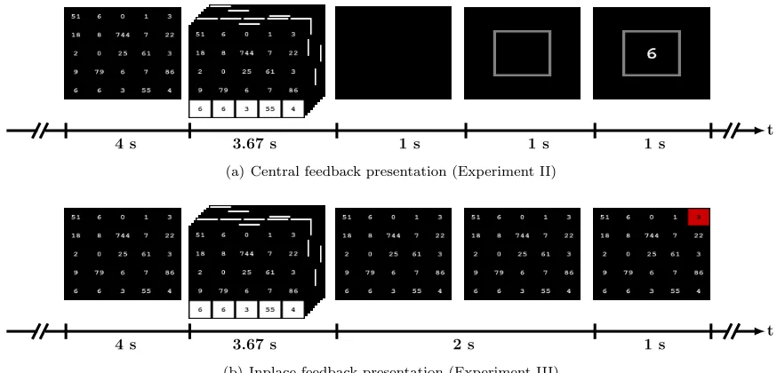
After a decision was made about the user intent in the online P300 sessions, flashing was stopped and the mask was completely emptied for a duration of one second. Then, an empty square was shown at the center of the display for one second, aiming at directing the user’s gaze to this location [30]. The estimated user intent (number) was shown afterwards inside the square for another second. The time between the end of the last flash and the presentation of the estimated number was therefore 2 seconds. Figure 4(a) shows the key events in a single ErrP/noErrP trial. Each subject underwent a different number of sessions, each consisted of a different number of ErrP/noErrP trials. It is noteworthy here that the P300 training and online sessions differ with respect to the task (spelling vs. finding maximum number) and the matrix size (6x6 vs. 5x5). Hereby, the straightforward classifier transfer across these sessions confirms previous findings that P300-based BCIs generalize across different operational tasks [39, 41, 55, 56], and across different matrix sizes [57].
3.3.3. Experiment III: P300-based interaction with inplace feedback
This experiment shared all details of Exp. II except the way the feedback was shown to users. Hereby, the mask remained displayed after flashing was stopped for 2 s and the estimated number was then highlighted for 1 s with a red square as shown in figure 4(b). After highlighting the estimated number, the P300 matrix was updated with a new set of random numbers.
3.3.4. Interrelation among experiments
Exp. II and III differ only with respect to the style of feedback presentation. On the one hand, should the central method be used for feedback presentations as in Exp. II, subjects need to test whether the presented number is a 3-digit number or not. On the other hand, to assess the correctness of interface actions in case of Exp. III, no comparison is necessary, as noticing that the visual feedback is shown on the P300 matrix over a place that does not match the previously attended one is sufficient to realize that an error has occurred. Thus, the feedback presentation in erroneous trials in this case is expected to be the target of a rapid eye movement (i.e. saccade). About 200 ms [58] are typically required for the eye to make such a movement. For correct trials, the feedback is shown overlaid on the previously fixated number, and therefore no saccades are expected to take place. It can be argued for Exp. III, therefore, that the processing of the feedback stimuli in case of erroneous trials starts at a later point in time compared to correct ones.
Obviously, the two feedback strategies in Exp. II and III require different mental processes to arrive at a decision whether the estimated number is correct or not. As such, these two experiments in particular enable us to examine invariance/variability ofinteraction ErrPs during P300-mediated interaction with respect to the required mental processing.
1 s 1 s
1 s 3.67 s
4 s t
(a) Central feedback presentation (Experiment II)
1 s 2 s
3.67 s
4 s t
[image:9.612.83.520.61.271.2](b) Inplace feedback presentation (Experiment III)
Figure 4: Key events in experiments II and III. The flashing time (3.67 s) is shown as an example for the case when two flashing repetitions were used.
respect to the user input (keyboard vs. P300), where we also introduced about 1 s delay between the user input and the feedback onset in Exp. I and 2 s in Exp. II and III. The 1 s delay in Exp. I and the 2 s delay in Exp. II are sufficient to respectively isolate hand-movement and eye-movement-related potentials. The 2 s delay in Exp. III was chosen to match that of Exp. II. Supported by the remarks from subsection 2.2, the main difference in our understanding between the different experiments, is the mental processing required to assess the movement of the ball in Exp. I compared to the processing of the central and inplace feedback in the P300-based interaction experiments. Furthermore, the presence of EOG artifacts that accompany feedback onset in Exp. I will be useful to understand the effect of these artifacts in Exp. I and III.
3.4. Classification
Two binary classification problems are encountered within this work with the goal of discriminating between target and nontarget flashes (in Exp. II and III) and between single trial ErrP and noErrP (in all experiments). In both cases, the goal is to find a mapping function h : X → Y, that maps from the domain of thed-dimensional feature spaceX =Rd to
the range of class labelsY ={ω1, ω2}.
In supervised classification methods,h is learned from a training dataset (D) containing n = n1+n2 tuples of observations and their labels, i.e.
D={(x(1), h(x(1))),(x(2), h(x(2))),
· · ·(x(n), h(x(n)))
},
where h(x(i)))
∈ {ω1, ω2} ∀i, and n1 and n2 are the number of available examples for class ω1 and ω2, respectively. LDA assumes two normal distributions for the two classes, such that x|ω1 ∼
N(µ1,Σ1),x|ω2 ∼ N(µ2,Σ2), and that the two classes share a common covariance matrix (i.e. Σ1 =
Σ2 =Σ). The LDA-based mapping function can be computed with hLDA = sign(wTx+b), wherew and b to be learned from D with class labels mapped to
ω1 = 1, ω2 = −1. The weighting vector can be computed with w =Σ−1(µ
1−µ2) and the bias with
b=−1
2 (µ1+µ2)Tw.
Since the true means and covariance matrices for each class are unknown, estimates thereof are substituted for the computations of w and b. The sample means are computed with ˆµ1 = 1
n1 Pi=n1
i=1 x (i) and ˆµ2 = 1
n2 Pi=n
i=n1+1x
(i), and the pooled sample covariance matrix is computed with
ˆ
Σ = 1
n−2
h
(n1−1) ˆΣ1+ (n2−1) ˆΣ2
i
, where ˆΣ1 and ˆ
Σ2 are the within-class sample covariance matrices, which can be estimated with
ˆ
Σ1 = n1−11P
i=n1
i=1 (x (i)
− µˆ1)(x(i)
− µˆ1)T and
similarly for ˆΣ2. These estimates of the covariance matrices are known as the maximum likelihood (ML) estimates, which fail to provide invertible ˆΣ when
shrinkage-LDA. The former is used to classify P300 trials (since
n1, n2> d) and the latter is used to classify ErrP trials (as fewer number of trials were acquired especially for Exp. II and III).
3.5. Pre-processing and feature extraction pipeline
Pre-processing and feature extraction of P300 and ErrPs differ fundamentally as a result of differences in their spatial, temporal and spectral characteris-tics. The P300 pipeline used here is based on pre-vious works [62, 63] that have shown good classifica-tion/spelling accuracies with LDA classifiers, and was decided upon before our recordings took place to fa-cilitate discriminating target and nontarget trials in online P300 sessions. The ErrP pipeline was, on the other hand, adopted post hoc to facilitate our offline analysis.
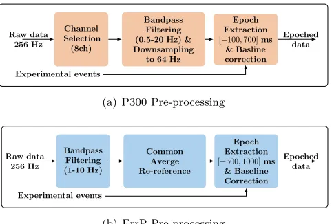
3.5.1. P300 pre-processing and feature extraction Only a subset of the EEG electrodes (Fz, Cz, P3, Pz, P4, PO7, POz and PO8) were used for P300 classification during experiments II and III, since P300 is believed to have a central and parietal distribution. Additionally, EEG data from these electrodes were shown to lead to relatively good P300 classification accuracies [64]. The continuous raw data from these 8 electrodes were notch-filtered at 50 Hz, bandpass-filtered with a 4thorder butterworth filter in the range
0.5 −20 Hz (since P300 is believed to be composed of phase-locked delta, theta and alpha oscillations [65– 68]) and downsampled to 64 Hz.
Event-locked EEG epochs of 800 ms duration were extracted from the pre-processed continuous data about the onset of each target/nontarget flash, i.e. a baseline of 100 ms pre-stimulus and 700 ms post-stimulus. The temporal mean of the baseline at each electrode was then subtracted from the post-stimulus data. A schematic of this pre-processing pipeline is depicted in figure 5(a).
Features per electrode were obtained by downsam-pling the epoched data with a factor of 3, and features from the 8 electrodes were finally concatenated to form the labeled feature vectors (with a resulting dimensio-nality of 8× d0.7×64/3e = 120). Each training ses-sion produced respectively around 160 and 800 target and nontarget training trials, which were used to train an ML-LDA classifier. In online sessions, feature vec-tors were obtained with the same pre-processing and feature extraction pipeline, where the unknown label of each feature vector was estimated with the learned ML-LDA classifier. Noteworthy here is that we did not aim at optimizing the accuracy of the P300-based in-teraction during the performed experiments (e.g. by using shrinkage-LDA to classify target/nontarget flas-hes [37] or by optimizing the number of repetitions),
Channel Selection
(8ch)
Bandpass Filtering (0.5-20 Hz) & Downsampling
to 64 Hz
Epoch Extraction [−100,700]ms
& Basline correction
Experimental events Raw data
256 Hz
Epoched data
(a) P300 Pre-processing
Bandpass Filtering (1-10 Hz)
Common Averge Re-reference
Epoch Extraction [−500,1000]ms
& Baseline Correction Raw data
256 Hz
Experimental events
Epoched data
[image:10.612.313.554.59.222.2](b) ErrP Pre-processing
Figure 5: The different pre-processing and epoch extraction pipelines for P300 and ErrP. Feature extraction is performed on the epoched data.
but rather at collecting as many ErrP and noErrP single trials as possible, with a reasonable number of flashing repetitions.
3.5.2. ErrP pre-processing and feature extraction The continuous EEG data from all 28 electrodes were first bandpass-filtered with a 4th order butterworth
filter in the range 1−10 Hz (since ErrP is believed to be relatively slow cortical potentials [12,42,69]) and then re-referenced to the common spatial average (i.e. the spatial mean was subtracted from each channel) to enhance SNR. EEG epochs in the period [−0.5,1.0] s time-locked to the feedback onset were extracted from the pre-processed EEG data and corrected for the 500 ms pre-stimulus baseline (i.e. the temporal mean of the baseline data was subtracted from the post-stimulus data). This pipeline is schematically shown in figure 5(b).
Features per electrode were obtained by downsam-pling the epoched data by a factor of 8. Feature vectors were then obtained by concatenating features in the time region [0.15,1] s following the feedback onset from the 5 midline electrodes (Fz, FCz, Cz, CPz and Pz), re-sulting in a dimensionality of 5× b0.85×256/8c= 135. Hereby, the selection of the midline channels is sup-ported by the fact that ErrPs exhibit a fronto-central distribution along the midline [12] and that features from the central brain regions result in superior clas-sification accuracy when compared to the peripheral regions [51].
3.6. Analysis of interaction ErrP invariance and variability
from EEG epochs of 1.5 s duration extracted about the feedback onset consisting of 0.5 s pre-stimulus and 1 s post-stimulus data. We base our analysis hereby mainly on the grand EEG average (i.e. the average over subjects) of the correct and error trials, to which we will refer respectively as the GAC, GAE. The grand average difference waveform (i.e. GAD) is simply the difference between GAE and GAC. All waveforms will be shown for either the frontocentral electrode FCz or the vertex (i.e. Cz), since several studies have poin-ted out a strong role of the ACC and adjacent fronto-central brain areas in monitoring errors [70].
Epochs, which contained, within the first post-stimulus second, EEG potentials outside the range
±50µV or EOG potentials outside the range ±200µV were excluded from the average computation, aiming at preventing strong ocular (e.g. eye blinks) artifacts from appearing in the average signals.
Statistical analysis of the difference between GAE and GAC signals within each experiment is performed using the adaptive factor adjustment procedure described in [71], controlling for the false discovery rate (FDR) at the 0.05 level. To this end, the functionerpfatestfrom RERPpackage is used.
Additionally, the signed r2 discriminability test [41, 72] is performed on correct and error trials of each subject in order to highlight the major spatial and temporal sources of variance among them within the different experiments. Intuitively, the unsignedr2 quantifies the proportion of the total amplitude vari-ance that is explained by the ground truth labels of the acquired sample data. Formally, it is computed for a certain feature with
r2k=
cov(xk,ω)2
var(xk) var(ω), (1)
where the vectorωis constructed from all the sample labels, i.e. ω= [h(x(1)), h(x(2)),
· · ·h(x(n))]T andxk is
constructed by concatenating thekthelement of thed
-dimensional feature vectors. The signedr2is computed withr2
·sign (cov (xk,ω)). Similar to [11],r2is used to assess the signal-to-noise ratio (SNR) of the different ErrP peaks.
3.6.2. ErrP classification: A 10-fold cross-validation was used to evaluate the performance of the shrinkage-LDA classifier in predicting the correct (noErrP) and incorrect (ErrP) trials obtained during the different experiments. In order to better estimate the classification accuracy in online sessions, all extracted trials, including the ones with strong ocular artifacts, were used for the classifier training and testing. Accuracy is reported in terms of the true positive rate (TPR or sensitivity) and true negative rate (TNR or specificity), which respectively reflect the rate of correct decoding of erroneous and correct
trials. The different experimental tasks produce imbalanced data sets (i.e. numbers of ErrP and noErrP trials are different), typically resulting in biased classification towards the majority class [51]. As a remedy, the normalized mutual information (NMI) [2] was additionally adopted as a single metric that incorporates both sensitivity and specificity. The reader is referred to [2] for the exact definition of NMI and its computation procedure, but it is important to note that NMI lies between 0 and 1, with the values 0 and 1, respectively reflecting chance-level (i.e. no class structure is found by the classifier) and perfect classification accuracy.
Furthermore, in order to quantify the invariance in ErrPs with respect to the different experimental factors (subjects, time and mental processes required to assess interface actions), the accuracy of classifier transfer across the different levels of these factors are reported. In particular, with respect to subjects, we choose to use per-experiment leave-one-subject-out cross validation method, where data from all subjects but one are used to train a classifier, which is then applied on the data of the left-out subject. The procedure is repeated separately for each experiment. On the other hand, with respect to time, we choose to use per-experiment and per-subject cross-day validation method, where the data from a specific subject/recording is used to test a classifier that is trained using data acquired from a previous recording of the same experiment. Finally, with respect to the mental processing, per-subject leave-one-experiment-in cross validation [73] is used. Hereby, the data from each experiment is used to train a classifier which is then applied on the data from each other experiment. This procedure is repeated for each subject.
In order to assess the significance of the obtained accuracies (quantified with NMI), p-values were obtai-ned using the label randomization test procedure [74], where 1000 permutations were performed in total. P-values below 0.05 are considered to be statistically sig-nificant, i.e. rejecting the null hypothesis that the data and class labels are independent, that is, there is no difference between the classes [74].
4. Experimental results
4.1. Datasets
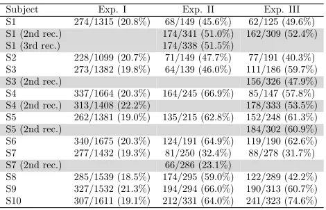
Table 1: Number of extracted trials written in the form (Number of ErrP trials/Total number of trials). Percentage of ErrP to total trials is shown in parentheses.
Subject Exp. I Exp. II Exp. III
S1 274/1315 (20.8%) 68/149 (45.6%) 62/125 (49.6%)
S1 (2nd rec.) 174/341 (51.0%) 162/309 (52.4%)
S1 (3rd rec.) 174/338 (51.5%)
S2 228/1099 (20.7%) 71/149 (47.7%) 77/191 (40.3%)
S3 273/1382 (19.8%) 64/139 (46.0%) 111/186 (59.7%)
S3 (2nd rec.) 156/326 (47.9%)
S4 337/1664 (20.3%) 164/245 (66.9%) 85/147 (57.8%)
S4 (2nd rec.) 313/1408 (22.2%) 178/333 (53.5%)
S5 262/1381 (19.0%) 135/215 (62.8%) 152/248 (61.3%)
S5 (2nd rec.) 184/302 (60.9%)
S6 340/1675 (20.3%) 124/191 (64.9%) 119/190 (62.6%)
S7 277/1432 (19.3%) 81/250 (32.4%) 88/278 (31.7%)
S7 (2nd rec.) 66/286 (23.1%)
S8 285/1539 (18.5%) 174/295 (59.0%) 122/289 (42.2%)
S9 327/1532 (21.3%) 194/294 (66.0%) 190/313 (60.7%)
S10 307/1611 (19.1%) 212/331 (64.0%) 241/323 (74.6%)
4.2. Neurophysiological analysis
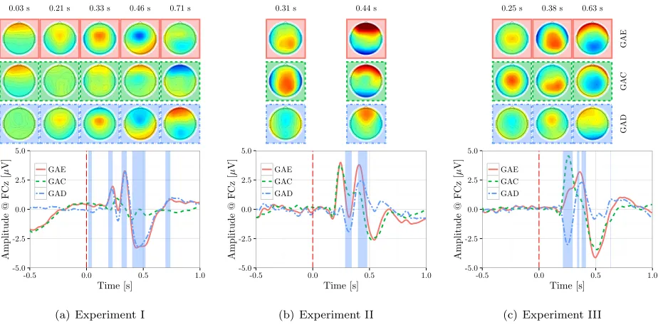
4.2.1. Experiment I: The GAC, GAE and GAD for Exp. I are shown in figure 6(a). The GAD exhibits an early positivity around 220 ms (P2), early negativity around 280 ms (N2) followed by a positivity around 340 ms (P3) and a later wider negativity around 460 ms (N4). Following the adaptive factor adjustment procedure [71], the difference was found to be significant around all the observed peaks except for the N2. Visual inspection of the GAE and GAC waveforms reveals that the P3 and N4 deflections are specific to error trials. The SNR value and the peak latency of these GAD peaks for each subject/recording are reported in table 2.
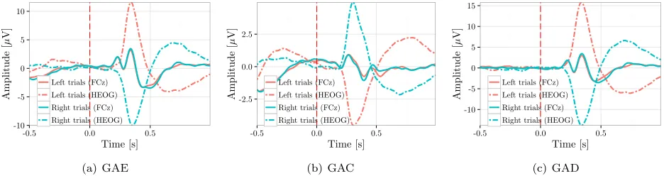
Furthermore, since the correct direction of the ball movement in Exp. I was randomly alternating between the right and the left direction with each new run, correct and incorrect trials for these two conditions obviously result in different HEOG traces. This can be seen in figure 7, where the average HEOG traces were plotted separately for the right and left trials alongside the GAC, GAE and GAD waveforms. Hereby, all average waveforms are computed by averaging an equal number of left and right trials for each subject. The observed discrepancy in the HEOG traces, did not propagate to the electrode site FCz, as one can hardly observe any difference in the GAC, GAE, GAD waveforms computed separately for the two directions. These results are in agreement with [12] and find support in [75], where it is argued that horizontal eye movement have no effect on the central sites.
4.2.2. Experiment II: The GAD waveform at FCz, plotted in figure 6(b), is characterized with a negative peak (N) at around 330 ms and a later positive peak (P) at around 430 ms. Visual inspection of the GAC
and GAE waveforms reveals that these two deflections are particularly present in error trials. Further, the time regions around these peaks are identified to be statistically significant following the adaptive factor adjustment procedure [71]. Per subject SNR and peak latency of the two peaks are presented in table 2.
4.2.3. Experiment III: The GAD waveform at FCz, plotted in figure 6(c), is characterized by a negative peak (N) at around 260 ms and a later positive peak (P) at around 380 ms. The peak amplitudes and latencies of the two peaks are reported for each subject/recording in table 2. Visual inspection of the GAE and GAC shows that both waveforms are characterized with a positivity and a later negativity. A Wilcoxon paired rank sum test (p= 0.064) revealed a trend toward a difference in the latency of the positivity between the GAE and GAC. This difference is estimated to be around 0.05 s and might be attributed to the extra time required to notice the flash on the screen in case of error trials. As such, this delay is likely to be, as well, the source of the two deflections in the GAD waveform.
Arguably, the activity at the FCz site in case of errors after t = 0 cannot be explained by the ocular artifacts (or saccades) that accompany these errors, since similar activity, yet with a different peak latency, is observed in correct trials where no eye movement is required.
4.3. Within-experiments Classification Results
-5.0 -2.5 0.0 2.5 5.0
-0.5 0.0 0.5 1.0
Time [s]
Amplitude
@
F
Cz
[
µ
V] waveformGAE
GAC GAD
0.03 s 0.21 s 0.33 s 0.46 s 0.71 s
(a) Experiment I
-5.0 -2.5 0.0 2.5 5.0
-0.5 0.0 0.5 1.0 Time [s]
Amplitude
@
F
Cz
[
µ
V] waveformGAE GAC GAD
0.31 s 0.44 s
(b) Experiment II
-5.0 -2.5 0.0 2.5 5.0
-0.5 0.0 0.5 1.0
Time [s]
Amplitude
@
F
Cz
[
µ
V] waveformGAE GAC GAD
0.25 s 0.38 s 0.63 s
GAE
GA
C
GAD
[image:13.612.74.536.65.295.2](c) Experiment III
Figure 6: The GAC, GAE and GAD waveforms were computed from the average of all subjects and recordings for all experiments. The shaded areas represent significant time regions in GAD as identified with the adaptive factor adjustment procedure described in [71]. Scalp topographies of voltage amplitudes (averaged over the significant time regions) are plotted in the upper panel.
Table 2: Per-subject SNR (r2) and latency values for the different peaks of the GAD waveform in the three experiments. Shaded rows highlight the second and third recordings of subjects who perfomed one experiment (or more) mutliple times. The coefficient of variation (CV) of each column is tabulated in the last row.
Experiment I Experiment II Experiment III
P3 N4 N P N P
Subject SNR (r2) Latency SNR (r2) Latency SNR (r2) Latency SNR (r2) Latency SNR (r2) Latency SNR (r2) Latency
S1 0.259 0.36 0.157 0.46 0.289 0.31 0.230 0.39 0.251 0.27 0.208 0.35
S1 (2nd rec.) 0.057 0.31 0.131 0.38 0.234 0.25 0.058 0.37
S1 (3rd rec.) 0.073 0.32 0.096 0.38
S2 0.218 0.34 0.182 0.44 0.039 0.33 0.084 0.43 0.058 0.25 0.241 0.37
S3 0.037 0.34 0.029 0.42 0.159 0.30 0.252 0.39 0.420 0.25 0.263 0.39
S3 (2nd rec.) 0.277 0.25 0.167 0.38
S4 0.003 0.39 0.007 0.52 0.190 0.35 0.206 0.46 0.231 0.25 0.163 0.40
S4 (2nd rec.) 0.007 0.33 0.009 0.57 0.154 0.25 0.087 0.40
S5 0.091 0.37 0.049 0.47 0.010 0.37 0.013 0.50 0.039 0.24 0.002 0.37
S5 (2nd rec.) 0.048 0.25 0.029 0.35
S6 0.013 0.32 0.135 0.44 0.021 0.34 0.173 0.54 0.009 0.26 0.081 0.42
S7 0.029 0.36 0.057 0.45 0.015 0.32 0.101 0.40 0.089 0.30 0.109 0.38
S7 (2nd rec.) 0.051 0.32 0.204 0.38
S8 0.074 0.34 0.064 0.43 0.099 0.35 0.159 0.45 0.131 0.27 0.027 0.34
S9 0.086 0.35 0.087 0.49 0.050 0.34 0.112 0.47 0.153 0.27 0.007 0.33
S10 0.308 0.34 0.256 0.45 0.016 0.29 0.009 0.39 0.050 0.27 0.103 0.43
mean±std 0.102±0.11 0.35±0.02 0.094±0.08 0.47±0.04 0.082±0.08 0.33±0.02 0.136±0.08 0.43±0.05 0.153±0.12 0.26±0.01 0.110±0.09 0.38±0.03
CV 1.06 0.06 0.85 0.10 1.01 0.07 0.56 0.12 0.76 0.06 0.78 0.08
4.4. Invariance and variability in ErrPs with respect to subjects
Figure 8 shows per-subject average difference waveform separately for each experiment. The variability across subjects is also shown with the shaded area, representing the standard error of the mean. From these plots and the results in table 2, one can observe inter-subject variability with respect to the amplitudes and SNR of the different deflections. The timing of the different deflections, however, seems to be more consistent across subjects as indicated by the values of the coefficient of variation (i.e., the standard deviation
divided by the mean) reported in the last row of table 2. As in [51], it can be argued that the high variance of classification accuracy across subjects, reported in table 3, can be attributed to the fact that these subjects have different concentration levels on the performed tasks.
-10 -5 0 5 10
-0.5 0.0 0.5
Time [s]
Amplitude
[
µ
V]
Left trials (FCz) Left trials (HEOG)
Right trials (FCz) Right trials (HEOG)
(a) GAE
-2.5 0.0 2.5
-0.5 0.0 0.5
Time [s]
Amplitude
[
µ
V]
Left trials (FCz) Left trials (HEOG)
Right trials (FCz) Right trials (HEOG)
(b) GAC
-10 -5 0 5 10 15
-0.5 0.0 0.5
Time [s]
Amplitude
[
µ
V]
Left trials (FCz) Left trials (HEOG)
Right trials (FCz) Right trials (HEOG)
[image:14.612.70.538.67.191.2](c) GAD
Figure 7: The GAE, GAC and GAD waveforms computed from equivalent number of left and right trials per subject in Exp. I at the electrode site FCz and for HEOG.
-6 -3 0 3 6
0.00 0.25 0.50 0.75 1.00 Time [s]
Amplitude
@
F
Cz
[
µ
V]
(a) Experiment I
-3 0 3 6
0.00 0.25 0.50 0.75 1.00 Time [s]
Amplitude
@
F
Cz
[
µ
V]
(b) Experiment II
-4 0 4
0.00 0.25 0.50 0.75 1.00 Time [s]
Amplitude
@
F
Cz
[
µ
V]
(c) Experiment III
Figure 8: The average difference (error-minus-correct) waveform plotted for each subject in Exp. (a) I, (b) II and (c) III. Shaded area represents the standard error estimate across the different subjects.
all subjects Exp. I and 70% of all subjects in Exp. II and III. However, it can be easily seen that the obtained NMI values are inferior to the cross-validation accuracies obtained for each subject/experiment listed in table 3. The differences were observed to be 0.09, 0.2 and 0.22, respectively for Exp. I, II and III. These differences were revealed to be significant with Wilcoxon paired rank sum tests, applied separately for each experiment on the data tabulated in table 3 and table 4, and corrected for multiple tests using the Benjamini-Hochberg false discovery rate control procedure [76]. Corrected p-values were (p = 0.002) for all experiments.
Altogether, these results suggest that despite inter-subject variability that negatively affects classi-fier transfer performance, invariant features across sub-jects can be obtained.
4.5. Invariance and variability in ErrPs over time
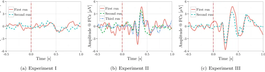
Figure 9 shows the GAD waveforms computed for the participants S4, S1 and S3 who completed multiple recordings for experiments I, II and III, respectively. Visual inspection of these plots shows that the shapes of the ErrPs are empirically invariant over time for the
same experiment/interface/subject. This observation which is valid for all our three interfaces agrees with [12], where the same is shown using an interface very similar to the one in Exp. I. Combined with the results in table 2, it can be observed that the SNR, amplitude and latency of the different peaks are quite stable over time.
[image:14.612.79.537.247.373.2]-6 -3 0 3 6
-0.5 0.0 0.5 1.0
Time [s]
Amplitude
@
F
Cz
[
µ
V] dayFirst run
Second run
(a) Experiment I
-6 -3 0 3 6
-0.5 0.0 0.5 1.0
Time [s]
Amplitude
@
F
Cz
[
µ
V]
day First run Second run Third run
(b) Experiment II
-6 -3 0 3 6
-0.5 0.0 0.5 1.0
Time [s]
Amplitude
@
F
Cz
[
µ
V] dayFirst run
Second run
[image:15.612.77.539.66.192.2](c) Experiment III
Figure 9: Examples of the GAD waveforms computed for the different experiments for some subjects who performed one experiment or more on multiple occasions.
than over subjects for the same experiment/interface, which is also supported by the similar GAD waveforms obtained for the different days.
4.6. Invariance/variability with respect to human mental processing of interface actions
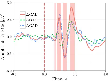
In section 4.2, we have compared the GAE and GAC waveforms to reason about the observed components in the GAD waveform for each experiment. In the follo-wing, we compare the GAE and GAC waveforms across experiments to reason about the variability/invariance in the computed GAD waveforms with respect to the mental processing required to assess the interface acti-ons. To this end, figure 10 rearranges the GAE, GAC and GAD waveforms from figure 6 and plots them over experiments.
4.6.1. Experiment II vs. III
As can be seen from figure 10(c) and table 2, both the GAD waveforms of Exp. II and III are characterized by a negativity and a later positivity. Further, from figure 6 and other results in section 4.2 ,we have seen that not only the timing of the two deflections varied across experiments, but also their relation to the time course of the GAC and GAE waveforms. In Exp. II, the two ErrP deflections in the GAD were primarily present in error trials, whereas in Exp. III, the deflections might have appeared as a result of the time delay in processing the error trials relative to the correct ones. The different mental processes required to evaluate the interface actions, as has been discussed in 3.3.4, might provide a plausible explanation to this variability. It can be seen from figures 10 and 11 that the difference in the GAE waveforms across experiments is larger than that in the GAC waveforms. This additionally might hint at a role of the mental processing in the observed variability.
4.6.2. Experiment I vs. II
The discrepancy in the GAD waveform between Exp. I and Exp. II has been already observed in the literature, e.g. Sp¨uler and Niethammer note that the first positive peak and the N4 is not visible in interaction ErrPs for all BCI tasks [42]. In the current work, and by analyzing figure 6, we have additionally seen that the P3 and N4 deflections in the GAD waveform of Exp. I and the N and P deflections of Exp. II stem from their particular presence in error trials.
4.6.3. Per-subject across-experiments classifier trans-fer
The classification accuracies for the classifier transfer across the different experiments are listed in table 6. These results show that the classifier transfer between Exp. I and II, and between Exp. I and III provide in-significant and low accuracies for most subjects. The accuracies of the classifier transfer between Exp. II and III show significant results for almost half of the subjects.
5. Discussion
5.1. Significance of the results
-5.0 -2.5 0.0 2.5 5.0
-0.5 0.0 0.5 1.0
Time [s]
Amplitude
@
F
Cz
[
µ
V] expExp. I Exp. II Exp. III
(a) GAE
-5.0 -2.5 0.0 2.5 5.0
-0.5 0.0 0.5 1.0
Time [s]
Amplitude
@
F
Cz
[
µ
V] expExp. I Exp. II Exp. III
(b) GAC
-5.0 -2.5 0.0 2.5 5.0
-0.5 0.0 0.5 1.0
Time [s]
Amplitude
@
F
Cz
[
µ
V] expExp. I Exp. II Exp. III
[image:16.612.78.540.66.193.2](c) GAD
Figure 10: The GAE, GAC and GAD waveforms for the three experiments.
-5.0 -2.5 0.0 2.5 5.0
-0.5 0.0 0.5 1.0
Time [s]
Amplitude
@
F
Cz
[
µ
V]
waveform
∆GAE ∆GAC ∆GAD
Figure 11: The difference in GAE, GAC and GAD waveforms across Exp. II and III.
significant results for almost half of the subjects, where the results also show that the rate of correct detection of correct trials (TNR) is higher than that of incorrect trials (TPR). The later observation suggests that the similarity of the GAC waveforms in both experiments (i.e., II and III) may have contributed to these results. Furthermore, the relative invariance of ErrPs over time, and the identical pre-processing pipeline used for all experiments rule out their possible involvement in producing the observed variability across the different experiments. Conversely, it can be argued that should there be a considerable difference in the shape of the grand average error and correct trials across experiments/studies with the same tasks, different mental processes are expected to underly this difference. It cannot be said with certainty, however, that the observed variability in ErrPs can be fully accounted for by these factors. Variables like the structure/modality of the feedback, the pre-processing pipeline, the rarity/frequency of error occurrences [12], the severity of the error (i.e., the degree of mismatch between the actual outcome and user expectation) [77] and possible ocular and muscular artifacts may contribute as well to such variations, and
such contribution should be reduced as much as the experimental paradigms might allow.
Our results emphasize that different ErrP studies and the results obtained therefrom should be carefully compared, and a similarity in the GAD waveform should be always confirmed with respect to the separate averages of error and correct trials. For instance, the apparent similar shapes of the GAD waveforms in Exp. II and III might hint at a mere difference in latency between the peaks of the two signals. The larger signal difference in GAE between the experiments, as can be seen in figure 11, may rule out such explanation and instead, suggests a role of the different mental processing of the feedback stimuli. Furthermore, visual inspection of the average waveforms in Exp. II and III reveals the presence of the N4 component in both GAC and GAE waveforms, which was clearly absent in the GAD waveforms. Therefore, it would have been certainly misleading to just show the similarity of GAD waveforms in experiments II and III, or to claim that the late N4 component is specific to Exp. I.
In this work, we have investigated the invari-ance/variance of ErrPs mainly at the FCz electrode. Furthermore, despite the fact that ErrPs can be eva-luated in both the spectral and temporal domains, the focus of this study was laid upon the temporal domain and therefore no claim whatsoever about the spectral variability is made. Some evidence exists in the litera-ture, however, suggesting that the spectral responses to errors may vary as well with respect to different types of errors, e.g. between execution and outcome errors [42].
5.2. Comparison with relevant studies
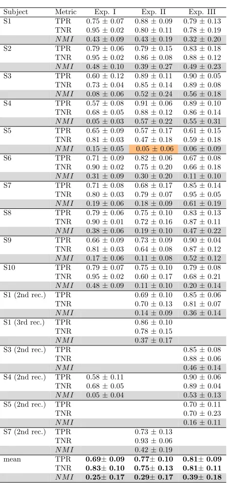
[image:16.612.85.275.236.378.2]Table 3: 10-fold cross-validation classification accuracy. Accuracy is reported in terms of TPR, TNR and NMI. All results were significant except for subject S5 in Exp. II.
Subject Metric Exp. I Exp. II Exp. III S1 TPR 0.75±0.07 0.88±0.09 0.79±0.13
TNR 0.95±0.02 0.80±0.11 0.78±0.19 N M I 0.43±0.09 0.43±0.19 0.32±0.20 S2 TPR 0.79±0.06 0.79±0.15 0.83±0.18 TNR 0.95±0.02 0.86±0.08 0.88±0.12 N M I 0.48±0.10 0.39±0.27 0.49±0.23 S3 TPR 0.60±0.12 0.89±0.11 0.90±0.05 TNR 0.73±0.04 0.85±0.14 0.89±0.08 N M I 0.08±0.06 0.52±0.24 0.56±0.18 S4 TPR 0.57±0.08 0.91±0.06 0.89±0.10 TNR 0.68±0.05 0.88±0.12 0.86±0.14 N M I 0.05±0.03 0.57±0.22 0.55±0.31 S5 TPR 0.65±0.09 0.57±0.17 0.61±0.15 TNR 0.81±0.03 0.47±0.18 0.59±0.18 N M I 0.15±0.05 0.05±0.06 0.06±0.09 S6 TPR 0.71±0.09 0.82±0.06 0.67±0.08 TNR 0.90±0.02 0.75±0.20 0.66±0.18 N M I 0.31±0.09 0.30±0.20 0.11±0.10 S7 TPR 0.71±0.08 0.68±0.17 0.85±0.14 TNR 0.80±0.03 0.79±0.07 0.95±0.05 N M I 0.19±0.06 0.18±0.09 0.61±0.19 S8 TPR 0.79±0.06 0.75±0.10 0.83±0.13 TNR 0.90±0.01 0.72±0.16 0.87±0.11 N M I 0.38±0.06 0.19±0.10 0.47±0.22 S9 TPR 0.66±0.09 0.73±0.09 0.90±0.04 TNR 0.81±0.03 0.64±0.08 0.87±0.12 N M I 0.17±0.06 0.11±0.08 0.52±0.12 S10 TPR 0.79±0.07 0.75±0.10 0.79±0.08 TNR 0.95±0.02 0.60±0.17 0.68±0.21 N M I 0.48±0.09 0.11±0.10 0.20±0.14 S1 (2nd rec.) TPR 0.69±0.10 0.85±0.06 TNR 0.70±0.13 0.81±0.07
N M I 0.14±0.09 0.36±0.14
S1 (3rd rec.) TPR 0.86±0.10
TNR 0.78±0.15
N M I 0.37±0.17
S3 (2nd rec.) TPR 0.85±0.08
TNR 0.88±0.06
N M I 0.46±0.14
S4 (2nd rec.) TPR 0.58±0.11 0.90±0.06 TNR 0.68±0.05 0.89±0.04
N M I 0.05±0.04 0.53±0.13
S5 (2nd rec.) TPR 0.70±0.11
TNR 0.70±0.23
N M I 0.16±0.11
S7 (2nd rec.) TPR 0.73±0.13
TNR 0.93±0.06
N M I 0.42±0.19
mean TPR 0.69±0.09 0.77±0.10 0.81±0.09
[image:17.612.61.296.110.608.2]TNR 0.83±0.10 0.75±0.13 0.81±0.11 N M I 0.25±0.17 0.29±0.17 0.39±0.18
Table 4: Leave-one-subject-out cross validation accuracies for each subject. Accuracies were significant except for the cells highlighted in orange.
Experiment I Experiment II Experiment III Sub. ErrP noErrP NMI ErrP noErrP NMI ErrP noErrP NMI
[image:17.612.313.544.301.408.2]S1 0.79 0.84 0.28 0.84 0.51 0.09 0.85 0.37 0.04 S2 0.82 0.84 0.32 0.87 0.53 0.13 0.77 0.75 0.19 S3 0.48 0.80 0.06 0.61 0.91 0.22 0.80 0.89 0.38 S4 0.44 0.75 0.03 0.63 0.88 0.20 0.82 0.68 0.19 S5 0.38 0.87 0.06 0.50 0.53 0.00 0.57 0.53 0.00 S6 0.38 0.95 0.14 0.81 0.27 0.00 0.93 0.15 0.01 S7 0.78 0.51 0.06 0.65 0.66 0.07 0.74 0.90 0.33 S8 0.80 0.70 0.16 0.65 0.73 0.10 0.54 0.86 0.13 S9 0.51 0.90 0.15 0.77 0.49 0.05 0.93 0.67 0.32 S10 0.83 0.85 0.33 0.54 0.58 0.01 0.80 0.49 0.07 mean 0.62 0.80 0.16 0.69 0.61 0.09 0.78 0.63 0.17
Table 5: Classification accuracies computed for the classifier transfer over time (NMIt) compared to the
10-fold cross validation NMI values from table 3. All results were identified as significant by the permutation test. The time gap (in days) between the different recordings is listed under ∆d.
Exp. Sub. Train w/ Test w/ ∆d NMI NMIt I S4 1st rec. 2nd rec. 3 0.05±0.04 0.04 II S1 1st rec. 2nd rec. 33 0.14±0.09 0.13 S1 1st rec. 3rd rec. 38 0.37±0.17 0.18 S1 2nd rec. 3rd rec. 5 0.37±0.17 0.19 S7 1st rec. 2nd rec. 6 0.42±0.19 0.30 III S1 1st rec. 2nd rec. 17 0.36±0.14 0.15 S3 1st rec. 2nd rec. 30 0.46±0.14 0.43 S4 1st rec. 2nd rec. 47 0.53±0.13 0.25 S5 1st rec. 2nd rec. 14 0.16±0.11 0.06
mean 0.32 0.19
the results from relevant studies in the literature. In particular, the interfaces in Exp. I and Exp. II have been previously used in the literature, and similar GAD waveform have been reported. Fig 12(a) compares the GAD obtained for Exp. I (solid line) and that in [12] (sparsely dashed line). We observe that the two waveforms exhibit high similarity with respect to their general shape, yet with a considerable variability with respect to the observed peak amplitudes and latencies. The shift in P3 latency was found to be significant;