Annual mean SST zonal section for the 2oN-2oS equatorial strip, for observations (GISST3) and for the CGCMs with no tropical flux adjustment(page 21).
More results of the CLIVAR Study of Tropical Oceans Intercomparisons Project (STOIC) can be found in the article by M. Davey et al. on page 21.
Note, that there are also results from the Coupled Model Intercomparison Project (CMIP) and the Paleo Climate Modelling Intercomparison Project (PMIP) in this issue.
Exchanges No. 17
The challenge of climate research: linking observations and models
Part 1: Ocean data assimilation and state estimation
Volume 5, No. 3
September 2000
Exchanges
Annual mean 2
o
N 2
o
S SST without flux correction
20
o60
o100
o140
o180
o220
o260
o300
o340
o380
oLongitude
20
25
30
35
Mean SST (Celcius)
GISST 1961 90 BMRC CCSR CERFACS
COLA ATL
COLA PAC
IPSL HR IPSL LR IPSL TOGA JMA
METO CM3
MPI
NCAR CSM ATL NCAR CSM PAC NCAR WM
Preliminary Announcement of Job Vacancies in the International CLIVAR Project Office (ICPO)
In September we expect to advertise internationally for staff scientists to work in the ICPO.
The staff appointed will work as members of the small team of scientists that supports the activities of CLI-VAR's panels and working groups and of its Scientific Steering Group. We will be seeking applications from sci-entists with relevant post-doctoral experience in atmos-pheric and/or ocean science and from those involved in the study of climate.
Duties will involve
• Developing, implementing and promoting CLIVAR sci-ence
• Working with national CLIVAR programmes to assess progress towards (and obstacles to) attaining CLIVAR objectives
• Helping to develop appropriate CLIVAR infrastructure particularly that needed for the effective management and distribution of CLIVAR-relevant data and prod-ucts
• Identifying and exploiting funding opportunities • Interacting with related research and operational
pro-grammes (e.g. IGBP, GCOS, GOOS, IHDP)
• Providing advice to the Director ICPO in the candidate's area of scientific expertise.
Note - It is expected that the staff appointed will be able to spend up to 20% of their time continuing their own CLIVAR-relevant research activity.
Conditions of employment
A successful candidate will become an employee of the University of Southampton on a salary scale depend-ing on qualification and relevant experience for an initial period of 3 years with the possibility of renewal.
The office is international and therefore candidates from outside the UK are encouraged to apply. Candidates should be able to write and speak English at an adequate level. The job will involve periods of overseas travel.
The ICPO is in the Southampton Oceanography Centre - a modern waterfront laboratory with a vibrant academic research atmosphere.
See http://www.soc.soton.ac.uk/ for more information. Please contact the Director ICPO ([email protected]) if you are interested in working in the ICPO and wish to receive further information.
Editorial
Dear CLIVAR community,
CLIVAR has global scope. Its complexity is increased by its synthesis of work from several disciplines, notably -meteorology, oceanography, hydrology, paleoclimatology and glaciology. Obervationalists, analysing instrumental as well as proxy data sets, are extending the climate record to provide new insights into today's climate and its rela-tionship to the past. Increasingly realistic climate models enable us to study mechanisms of natural climate variabil-ity as well as providing tools for short-term climate pre-dictions and projections of the human influence on climate. Observationalists and modellers depend on each other and on effective co-operation and communication across the disciplines. Without high quality observations model simulations and climate predictions are of limited use. However observations of all types are sparse and thus CLIVAR requires sophisticated data assimilation and syn-thesis techniques to bring observations and model simulations together.
Huge reanalysis efforts have already been under-taken and continue to improve our knowledge of the state of the atmosphere over the past decades. In the ocean how-ever such synthesis activities on a global scale are only just beginning. The triggers have been the large amount of in situ data that has been collected throughout the last dec-ades (e.g. under the auspices of WOCE), the availability of global satellite data sets (particularly altimetry) and the development of data assimilation techniques for ocean models. The Global Ocean Data Experiment (GODAE) part of the Global Ocean Observations System (GOOS) and WCRP-CLIVAR is one of the key projects in this context.
We invited the submission of brief articles on the syn-thesis of data and models to be published in Exchanges. There was an extremely encouraging response that clearly indicated a high level of interest and activity. Indeed the response was so great that we have been unable to include all contributions in a single issue. So we have split the con-tributions in a thematic way. This issue will mostly cover topics related to the ocean and the next one to be published in December will provide a more atmospheric view. Al-though this goes against our usual practice of integrating atmosphere and ocean as much as possible it seemed to be the only practical compromise I hope that you will enjoy these two issues.
Finally, I invite you to visit our re-designed web-site at http://www.clivar.org. We believe we have developed a much more user-friendly structure, containing more sci-ence and providing useful information for those who are new to CLIVAR as well as to those who are looking for detailed information. We hope that you will enjoy.
Detlef Stammer for the ECCO Consortium1
Scripps Institution for Oceanography, La Jolla, CA, USA [email protected]
1 D. Stammer (PI), R. Davis, L.-L. Fu, I. Fukumori, R.
Giering, T. Lee, J. Marotzke, J. Marshall, D. Menemenlis, P. Niiler, C. Wunsch, V. Zlotnicki
1. Introduction
The ocean is changing vigorously on a wide range of time and space scales. This variability leads to substan-tial problems in observing and modelling (simulating) the rapidly changing flow field, the ocean’s temperature dis-tribution, and more generally the consequences of those changes for climate. Prototype ocean observing systems, which are now in place as a legacy of programmes such as the World Ocean Circulation Experiment (WOCE) and the Tropical Ocean Global Atmosphere Programme (TOGA), aim at measuring and detecting large-scale changes of vari-ous quantities in the ocean, such as temperature, salinity, velocity, nutrients, tracers, etc. The present coverage of in-terior temperature and salinity measurements will signifi-cantly increase with the launch of the global ARGO float programme, which in combination with the complemen-tary high-quality altimetric satellite data will be the back-bone of a climate observing system. However, in spite of those unprecedented data, the interior of the ocean will remain fairly undersampled, and much of our understand-ing and inferences about the ocean’s role in shapunderstand-ing our climate will come from the additional information provided by numerical ocean general circulation models.
Among the goals of the present ocean and climate research are therefore to measure, understand, and even-tually predict these variations by combining ocean data and ocean models. Today high-resolution simulations of the ocean are performed on a routine basis with realistic coast-lines, bottom topography, and surface forcing. By combin-ing ocean observations with those state-of-the-art models, one can obtain an analysis of the time-varying ocean that, when taking into account errors in data and models, must necessarily be more complete and better than the informa-tion from either of them alone. This is the heart of ocean state estimation (often referred to as “data assimilation”) which has at its goal to obtain the best possible description of the changing ocean by forcing the numerical model so-lutions to be consistent with the observed ocean conditions. This by itself is a very cost-effective way to obtain a fairly complete description of the changing ocean from a limited set of observations. But at the same time it also identifies model components that need improvement, including sur-face forcing fields, and guides us as to where we need to extend the observing system to improve the estimated ocean state.
2. Ongoing Activities
Because of the fundamental importance of under-standing the present and future states of the ocean, two consortia on ocean modelling and state estimation were supported recently through the US National Ocean Part-nership Program (NOPP) with funding provided by the National Aeronautics and Space Administration (NASA), the National Science Foundation (NSF), and the Office of Naval Research (ONR). Those two modelling and assimi-lation activities are described in detail in Stammer and Chassignet (2000). One of them is called “Estimation of the Circulation and Climate of the Ocean” (ECCO). This ECCO consortium builds on existing efforts at the Massachusetts Institute of Technology (MIT), the Jet Propulsion Labora-tory (JPL), and the Scripps Institution of Oceanography (SIO), with additional partners at the Southampton Ocea-nographic Centre (SOC) and the Max-Planck Institut für Meteorologie (MPI) in Hamburg. Its primary goal is to pro-vide the best possible dynamically consistent estimates of the ocean circulation, which can serve as a basis for stud-ies of elements important to climate (e.g., heat fluxes and variabilities). This model-based synthesis and analysis of the large-scale ocean data set will enable a complete (i.e., including aspects not directly measured) dynamical de-scription of ocean circulation, such as insights into the na-tures of climate-related ocean variability, major ocean trans-port pathways, heat and freshwater flux divergences (simi-lar for tracer and oxygen, silica, nitrate), location and rate of ventilation, and of the ocean’s response to atmospheric variability.
The ongoing ocean state estimation is based on the MIT GCM (Marshall et al., 1997) and two parallel optimi-zation efforts: the adjoint method (Lagrange multipliers or constrained optimization method), exploiting the Tangent-linear and Adjoint Compiler (TAMC) of Giering and Kaminsky (1997) as described in Marotzke et al. (1999), and a reduced state Kalman filter, e.g., Fukumori et al. (1999). Those data assimilation activities can be summarized as finding a rigorous solution of the model state x over time t that minimizes in a least-squares sense a sum of model-data misfits and deviations from model equations while taking into account the errors in both.
First such results of a global ocean state estimation procedure are summarized in Stammer et al. (2000). Data currently employed in the optimization include the abso-lute and time-varying T/P data from October 1992 through December 1997, SSH anomalies from the ERS-1 and ERS-2 satellites, monthly mean sea-surface temperature data (Reynolds and Smith, 1994), time-varying NCEP reanalysis fluxes of momentum, heat, freshwater, and NSCAT esti-mates of wind stress errors. Monthly means of the model state are required to remain within assigned bounds of the monthly mean Levitus et al. (1994) climatology. To bring the model into consistency with the observations, the
tial potential temperature (θ) and salinity (S) fields are modified, as well as the surface forcing fields. Changes in those fields (often referred to as “control” terms) are deter-mined as a best-fit (in a least-squares sense) of the model state to the observations and their uncertainties over the full data period.
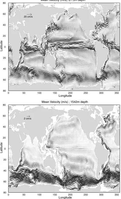
A few representative ECCO results are summarised in Fig. 1 and Fig. 2 (page 15). The estimated mean velocity field at 27 and 1542 m depth (Fig. 1) shows all major cur-rent systems. But with the low model resolution, they are necessarily overly smooth. The mean net surface heat and freshwater flux fields as they result from the optimization are displayed in the upper row of Fig. 2 (page 15). Their mean change relative to the prior NCEP fields are provided in the middle part of the figure. Ocean transports of all quantities are very energetic and variable. As an example we show here the net northward heat transport across 25oN
in the North Atlantic as it results from the optimized model state. The estimated time-varying model state, model trans-ports and consistent surface flux fields will be the basis for a wide variety of climate and societal applications. Many interdisciplinary applications are already under way or have begun recently, including studies of the ocean’s im-pact on the earth angular momentum budget (Ponte et al., 2000).
3. Outlook
Now ongoing computations move toward a 6-year estimate of the time-evolving ocean circulation (1992 through 1997) with 1o spatial resolution that uses all major
WOCE data sets as constraints, and that has build in a com-plete mixed layer model (Large et al., 1994) and an eddy parameterization scheme (Gent and McWilliams, 1990). It is anticipated that, in two to three years, the project will be able to address the US CLIVAR and GODAE related ob-jective of depicting the time-evolving ocean state with spa-tial resolution up to 1/4o globally and with substantially
higher resolution in nested regional approaches which are required for quantitative studies of the ocean circulation. Complementary to this, a 50 year long re-analysis experi-ment is anticipated but with only a 1o spatial resolution that
coincides with the NCEP/NCAR reanalysis period. A major issue for the ECCO consortium, and gener-ally for the wider oceanographic community, is the way in which the need for computer resources has now out-stripped their availability. No short-term solution to the computer resource bottleneck is as yet visible. However, there is an ongoing NOPP activity aiming to organise a substantial increase and improvement in computational in-frastructure for oceanographic research (OITI). If success-ful, it will have a profound impact not only on many fu-ture NOPP modelling and assimilation activities; it will be an important step toward reaching GODAE and CLIVAR goals.
The ECCO estimated time-varying model state and consistent surface flux fields from the entire estimation period can be accessed via the web page
http://www.ecco.ucsd.edu/.
References
Fukumori, I., R. Raghunath, L.-L. Fu, and Y. Chao, 1999: Assimi-lation of TOPEX/POSEIDON altimeter data into a global ocean circulation model: How good are the results? J. Geophys. Res., 104, 25,647–25,665.
Gent, P. R., and J.C. McWilliams, 1990: Isopycnal mixing in ocean models. J. Phys. Oceanogr., 20, 150-155.
Giering, R., and T. Kaminsky, 1997: Recipes for adjoint code con-struction. ACM Trans. Math. Software, 24, 437-474. Large, W. G., J.C. McWilliams, and S.C. Doney, 1994: Oceanic
ver-tical mixing: a review and a model with nonlocal bound-ary layer parameterization. Rev. Geophys., 32, 363–403. Levitus, S., R. Burgett, and T. Boyer, 1994: World Ocean Atlas 1994,
vol. 3, Salinity, and vol. 4, Temperature, NOAA Atlas NESDIS 3 & 4, U.S. Dep. of Comm., Washington, D.C. Marotzke, J., R. Giering, Q.K. Zhang, D. Stammer, C.N. Hill, and
T. Lee, 1999: Construction of the adjoint MIT ocean gen-eral circulation model and application to Atlantic heat transport sensitivity. J. Geophys. Res., 104, 29,529 - 29,548. Marshall, J., A. Adcroft, C. Hill, L. Perelman, and C. Heisey, 1997a: A finite-volume, incompressible navier-stokes model for studies of the ocean on parallel computers. J. Geophys. Res.,
102, 5753–5766.
Ponte, R. M., D. Stammer, and C. Wunsch, 2000: Improved ocean angular momentum estimates using an ocean model con-strained by large-scale data. Geophys. Res. Lett., submit-ted.
Reynolds, R. W., and T.M. Smith, 1994: Improved global sea sur-face temperature analyses using optimum interpolation. J. Climate, 7, 929–948.
Stammer, D., and E.P. Chassignet, 2000: Ocean State Estimation and Prediction in Support of Oceanographic Research. Oceanography, 13, 51–56.
Stephanie Guinehut, Gilles Larnicol, and Pierre-Yves Le Traon
CLS Space Oceanography Division, Ramonville St Agne, France
1. Introduction
The aim of the study is to analyse the contribution of different profiling float arrays [as proposed by the Argo project (Roemmich at al., 1999)] to the description of the variations of the large scale and low frequency 3-D thermohaline fields. It uses outputs and profiling float simulations from a primitive equation model of the North Atlantic Ocean.
2. Data and Method
2.1. Data
Model outputs and profiling float simulations from the MERCATOR project (Blanchet et al., 1999) are used. The model is a primitive equation model of the North At-lantic Ocean with a 1/3-degree horizontal resolution and 43 vertical levels. It uses realistic forcing from ECMWF reanalysis. The 1989-year simulation is used for the study.
2.2. Method
The objective is to reconstruct the large scale and low frequency variability of the temperature (T) and salinity (S) fields at different depths from simulated T and S pro-files corresponding to three-degree (“nominal” Argo reso-lution) Eulerian and Lagrangian arrays. The main issue is to analyze how an a priori defined large scale signal can be mapped from sparse measurements with a low signal-to-noise ratio (mainly due to mesoscale variability).
2.2.1. The reference fields
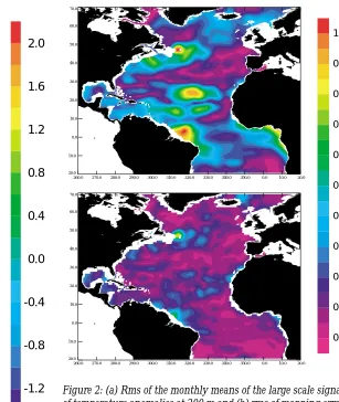
The first step consists in calculating the model large scale reference fields at different depths. Anomalies of the T and S fields relative to a five-year mean (1989 – 1993) are first calculated at each depth. The anomalies are then sepa-rated into a large scale part and a “mesoscale” part using a 2D Loess smoother (Greenslade et al., 1997) with a cut-off wavelength of 10° in latitude and longitude. This approxi-mately corresponds to averages over 6° by 6° boxes (Greenslade et al., 1997) and is supposed to be representa-tive of signals which can be mapped from a global profil-ing float array. An example is given in Figure 1 (page 16) for an instantaneous field of T at 200 m. The filter appears to preserve the main large scale features of the T and S fields while mainly removing the mesoscale signals. The large scale signal is the reference field which we want to reconstruct.
2.2.2. The objective analysis method
Simulated T and S profiles corresponding to three-degree Eulerian and Lagrangian arrays are subsampled from the model fields every ten days and at different depths (20, 200 and 1000 m). An objective analysis method (Bretherton et al., 1976) is then used to reconstruct the large scale signal variations from these simulated data.
The covariance functions of the large scale T and S signals at different depths are derived on a one degree by one degree grid from the analysis of the model large scale fields over the year 1989 (see figure 1-b). The model mesoscale signal (see figure 1-c) is used to determine the noise-to-signal ratio on the same grid. Thus, both covariance and noise-to-signal ratio depend on the geo-graphical position and on the depth. Values are very simi-lar for the T and S fields. Near the sea surface (20 m), the large scale signal dominates with low noise-to-signal ra-tios. Below the mixed layer depth, the large scale signal is, however, much smaller and the noise-to-signal ratio in-creases considerably. The noise-to-signal ratio varies from 0.1 at 20 m to 10 at 1000 m.
The analyses are performed every ten days over a one-year period (year 1989) but since the objective is to re-trieve the low frequency variability of the large scale sig-nal, monthly means are calculated. They are then compared to the monthly means derived from the model large scale reference fields.
3. Some statistical results for a three-degree Eulerian ar-ray
A three-degree regular Eulerian array (530 profiling floats over the area) is first tested for the T and S fields at 20, 200 and 1000 m. As an example, Figure 2 (page 16) shows the rms of the monthly means of the large scale T signal at 200 m and the rms of the mapping error obtained with the three-degree array. The rms of the mapping error is almost everywhere much smaller than the rms of the signal. The three-degree array captures the main large scale signal
Table 1 compares the mean mapping error (in rms and in percentage of signal variance) of the monthly means of the large scale T and S fields at different depths. Near the sea surface (20 m), the T field is a very large scale sig-nal with a large variance (rms = 2.08 °C). It corresponds to the SST response to the (large scale) atmospheric heat fluxes. This signal is almost perfectly retrieved with the three-degree array (99 % of the variance). The errors on the T signals decrease with depth (0.16 °C at 20 m to 0.14 °C at 200 m and 0.05 °C at 1000 m) but the T variance decreases much more rapidly (2.08 °C, 0.34 °C and 0.08 °C respec-tively at the same depths). As a result, the error relative to the signal variance increases considerably with depth. The
-Field Rms of mapping Mapping error in % error (°C) of signal variance
Temperature
20 m (2.08 °C) 0.16 0.6
200 m (0.34 °C) 0.14 17.5
1000 m (0.08 °C) 0.05 34.4
Salinity
20 m (0.19 psu) 0.05 7.4
200 m (0.06 psu) 0.02 15.8
[image:7.595.36.291.65.235.2]1000 m (0.01 psu) 0.008 28.3
Table 1: Mapping errors of the monthly means of the large scale temperature and salinity fields at different depths for the three-degree array (530 floats). The rms of the T and S sig-nals are also indicated.
Array Rms of mapping Mapping error in % error (°C) of signal variance
T at 200 m - signal variance = 0.34 °C
3°* 3° 0.14 17.6
Eulerian
3°* 3° 0.15 20.1
Lagrangian
Table 2: Mapping errors of the monthly means of the large scale temperature field at 200 m for the three-degree Eulerian and Lagrangian arrays.
three-degree array captures the main large scale signal at 200 m (82 % of the signal retrieved) but only 66% of the signal variance at 1000 m (table 1) due to the very low tem-perature variance at this depth. Results obtained for the S field are very similar to those obtained with the T field at 200 and 1000 m. Near the sea surface, salinity spatial scales are smaller than temperature ones and the signals are less easily reconstructed.
4. Comparison of Eulerian and Lagrangian arrays
Differences between Eulerian and Lagrangian three-degree arrays are now analysed. We used the Lagrangian float simulations at a 500 m depth. We chose to analyse the 500 m simulations (rather than 2000 m) to have a sufficient (and probably more realistic) estimation of the actual dis-persion of the floats.
The time evolution of the T mapping error at 200 m shows only a slight degradation of results for the Lagrangian array compared to the Eulerian array (not shown). Differences are of the order of 0.01 °C which is small compared to the signal variance. In only one year, the profiling floats did not disperse/converge much and all the floats continue to provide useful information. Part of the differences can actually be explained by the loss of 20 floats (which left the model domain) during this year.
5. Conclusions and perspectives
The study suggests that a three-degree array of pro-filing floats cycling every 10 days can retrieve most of the variance of the large scale and low frequency T and S sig-nals as observed by a 1/3° primitive equation model. More than 90 % of the variance of the T and S signals is retrieved at the surface (20 m), 80% at 200 m and between 65 and 70 % at 1000 m. Comparison between Eulerian and Lagrangian arrays shows only a slight degradation of the results due to the dispersion of floats.
These results depend, of course, on the a priori defi-nition of the large scale and low frequency signal (here space/time means over approximately 6°x 6° boxes and 1 month). Sensitivity studies to this a priori choice should be carried out to determine the mapping accuracy accord-ing to the space (e.g. from 3 degrees to 10 degrees) and time (e.g. from 10 days to one year) scales of signals to be mapped. Higher resolution models should also be used to better estimate the impact of the mesoscale field on the large scale signal retrieval. Finally, floats simulations over longer periods (4 years) should be used to better estimate the im-pact of the Lagrangian dispersion of the floats during their expected life-time.
Note, finally, that only profiling float data were used here to estimate the large scale T and S fields. It is clear, however, that in the future the best use of profiling float data will be when they are combined with other data sets and models through effective data assimilation techniques. The development and application of such techniques is the main (challenging) objective of GODAE (Smith and Lefebvre, 1997). The combination of profiling float data with satellite altimetry will be, in particular, very instrumental in reducing the aliasing due to the mesoscale variability.
Acknowledgements
We thank the MERCATOR PAM team for providing us with the model simulations. The study was partly funded by CNES under contract CNES/CLS 794/99/7805/ 00.
References
Blanchet, I., T. De Prada, Y. Drillet, L. Fleury, H. Perez, L. Siefridt, and B. Tranchant, 1999: The North Atlantic / Mediterra-nean Mercator Prototype. Oceanobs99. Conference proceed-ings, St Raphael.
Bretherton, F., R.E. Davis, and C.B. Fandry, 1976: A technique for objective analysis and design of oceanographic experi-ments applied to MODE-73. Deep-Sea Res., 23, 559-582. Greenslade D.J.M., D.B. Chelton, and M.G. Schlax, 1997: The
[image:7.595.38.293.641.742.2]Roemmich, D., O. Boebel, Y. Desaubies, H. Freeland, B. King, P.-Y. LeTraon, B. Molinari B. Owens, S. Riser, U. Send, K. Takeuchi, and S. Wijffels, 1999: Argo: The Global Array of Profiling Floats. Oceanobs99. Conference Proceedings, St Raphael.
Sigrid Schöttle and Mojib Latif,
Max-Planck-Institut für Meteorologie, Hamburg, Germany
Introduction
Successful El Niño forecasts depend on the avail-ability of suitable ocean initial states, especially from sub-surface layers. Sea sub-surface heights contain information about the ocean interior, and they can be measured with high accuracy from space. Here, we investigate the effect of the assimilation of TOPEX/POSEIDON sea surface heights on the oceanic initial conditions and the El Niño hindcast skill.
Several methods were developed to assimilate the sea surface heights (Cooper and Haines, 1996; Segschneider et al., 1999; Verron et al., 1999). Here we use an empirical method to project the sea surface heights on the vertical modes of the system. We have conducted an ensemble of El Niño hindcasts and forecasts with a hybrid coupled model. Our latest forecasts indicate the development of a weak El Niño towards the end of this year.
Models
Our forecast system consists of a hybrid coupled ocean-atmosphere model (HCM) and an ocean assimila-tion scheme described below. The ocean component of the HCM is a Pacific version of the HOPE-E model (Wolff et al., 1997), an ocean general circulation model based on primitive equations. Further details of the ocean model can be found in Venzke et al. (2000). The atmospheric compo-nent of the HCM is a statistical model (Barnett et al., 1993) which has been derived from a regression analysis of sea surface temperature and surface wind stress anomalies.
Forcing
The ocean model was forced by heat fluxes and wind stresses of two different data sets: a) NCEP reanalysis (Kalnay et al., 1996) for the period 1973-1997 and b) ECMWF re-analysis (ERA) and ECMWF operational analysis for the period 1990-June 2000. For the model runs with assimi-lation we used Topex/Poseidon data provided by CLS (Collecte Localisation Satellite). These data were already corrected and mapped (Le Traon et al., 1998). Up to Janu-ary 2000 we used historical homogeneous data on 10 day maps. Thereafter near real time data on 7 day maps were used which are available one week after their measurement.
Assimilation method
The assimilation method is similar to those of Fischer et al. (1997) and Mellor and Ezer (1991). Our approach con-sists of two steps. In the first step, the altimeter data were projected from the surface onto the vertical temperature structure at each grid point. This projection was realised by applying a transfer function that was computed from a regression between the sea level anomalies (SLA) and the principal components of the first two empirical orthogonal functions of the vertical temperature anomaly (TA) pro-file. The SLA and TA used to compute the regression were taken from a 45 year ocean model run forced by observa-tions. After the projection a mean seasonal cycle was added to yield full temperatures. In the second step, the model temperatures were nudged to these full temperatures at each time step with a relaxation time of about 4 days.
Results
Hindcasts were started every three months for the period 1993 to 1997. Sets of hindcasts were performed with and without assimilation of Topex/Poseidon data. Corre-lation coefficients of sea surface temperature anomalies (SSTA) averaged over the Niño-3 region were calculated between observations and hindcasts for time lags of 1 to 6 months (Fig.1). The assimilation of Topex/Poseidon data improved the skill of El Niño hindcasts considerably at all time lags.
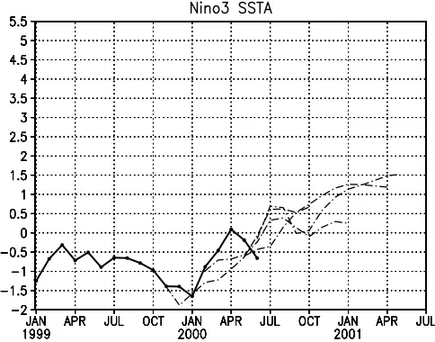
Our ocean analysis obtained by assimilating the Topex/Poseidon sea surface heights shows in June 2000 positive temperature anomalies at subsurface levels in the western equatorial Pacific. These are similar in magnitude to those simulated in December 1996 (Fig. 2). The anoma-lies in June 2000, however, are located slightly farther west relative to those in December 1996. We initialised forecasts in November 1999 and February, May and June 2000. Each forecast has a duration of 12 months. The results in terms of the Niño-3 SST index are shown in Fig. 3. The HCM predicts a mild El Nino for the winter season 2000/2001. One should keep in mind, however, that the model's skill drops rapidly beyond lead times of 6 months.
In summary, we can conclude that the assimilation of Topex/Poseidon sea surface heights improves signifi-cantly the skill of ENSO hindcasts. Future studies will in-volve the application of more sophisticated assimilation schemes and the inclusion of additional observations such as those measured by the TOGA-TAO array.
Smith, N., and M. Lefebvre, 1997:“The Global Ocean Data As-similation Experiment” (GODAE). Monitoring the oceans in the 2000s : an integrated approach, International Sympo-sium, Biarritz, October 15-17. 1997.
Fig. 1: Hindcast skill of Niño-3 SSTA index of a) persistence (black line), b) hindcasts without assimilation of T/P data (dashed dot-ted line) and c) hindcasts with assimilation of T/P data (dashed line).
Fig. 3: Niño-3 SSTA index of a) ECMWF SSTA data (black line) and forecasts initialised from an ocean model assimilation run (dashed-dot lines).
[image:9.595.139.453.328.761.2]Model Description
The model used is an intermediate resolution ver-sion of the Modular Ocean Model 3 (MOM3) code devel-oped at the National Oceanic and Atmospheric Adminis-tration’s Geophysical Fluid Dynamics Laboratory Pacanowski, 1995. The model’s spatial domain incorporates the Pacific basin from 120oE to 70oW and from 30oS to 30oN.
The grid resolution varies over the domain with the high-est resolution in the eastern equatorial region. The longi-tudinal resolution is a constant 0.5o from the eastern
bound-ary to 140oW. From 140oW to the western boundary the
lon-gitudinal resolution increases from 0.5o to 1.5o . The
latitu-dinal resolution is a constant 0.5o from 5oS to 15oN,
expand-ing poleward of this region to 1.5o at the southern and
north-ern boundaries. The resulting grid contains 241 points in longitude and 82 points in latitude. The model has 20 ver-tical layers with 10 equally spaced levels in the upper 150 meters. The model time step is one hour. The model em-ploys a Richardson number dependent mixing scheme in the vertical and a biharmonic mixing scheme in the hori-zontal. The model incorporates an optimal interpolation scheme which assimilates expendable bathythermograph (XBT) and mechanical bathythermograph (MBT) tempera-ture data from the NODC Levitus and Boyer (1994) data set, thermister data from the TOGA-TAO array of moor-ings in the Pacific and TOPEX/Poseidon satellite altimetry data when it became available in September 1992. The as-similation scheme and its incorporation into the model is described in detail by Carton et al., 1996. The model is forced with weekly NCEP winds Kalnay et al., 1996. Sea surface temperature (SST) is damped to NCEP weekly val-ues and the sea surface salinity (SSS) is damped to monthly
Acknowledgements
The altimeter products were produced by the CLS Space Oceanography Division as part of the DUACS (ENV4-CT96-0357) project. We thank M. Balmaseda for providing us with the ECMWF forcing data.
References
Barnett, T.P., M. Latif, N. Graham, M. Flügel, S. Pazan and W. White, 1992: ENSO and ENSO-related predictability. Part I: Prediction of equatorial Pacific sea surface temperature with a hybrid coupled ocean-atmosphere model. J. Climate,
7, 1513-1564.
Cooper, M., and K. Haines, 1996: Altimetric assimilation with wa-ter property conservation. J. Geophys. Res., 101, 1059-1077. Fischer, M., M. Flügel, M. Ji, and M. Latif, 1997: The Impact of Data Assimilation on ENSO Simulations and Predictions. Mon. Wea. Rev., 125, 819-829.
Kalnay, E., M. Kanamitsu, R. Kistler, W. Collins, D. Deaven, L. Gandin, M. Iredell, S. Saha, G.White, J. Woollen, Y. Zhu,
Howard F. Seidel, Texas A&M University, College Sta-tion, TX, USA
Benjamin Giese, Texas A&M University, College Sta-tion, TX, USA
Jim Carton, U. Maryland, College Park, MD, USA
Abstract
A medium resolution ocean general circulation model (OGCM) is used to explore current structure and variability in the equatorial Pacific for the period from 1992-1997. The model assimilates surface and subsurface tem-perature data from expendable bathythermographs (XBT), the Tropical Ocean Global Atmosphere-Tropical Atmos-phere-Ocean (TOGA-TAO) moorings and altimetry data from the TOPEX/Poseidon satellite. Model experiments are run with and without the assimilation of TOPEX/Poseidon altimetry observations in order to study their impact on model currents. Assimilated currents are compared with observed currents from the TOGA-TAO moorings at 110oW,
140oW and 165oE. Since mooring data are not assimilated,
these data provide an independent verification of the model results. The comparison shows that the model produces accurate equatorial currents over a wide range of spatial and temporal scales. In particular, the model correctly re-solves temporal variability from instability waves with periods of less than a month to interannual changes with periods of several years. A statistical analysis is conducted to quantify the model’s skill in producing accurate currents and to evaluate the importance of TOPEX/Poseidon altimetry assimilation.
The impact of TOPEX/POSEIDON altimetry assimilation on equatorial circulation modelling in the Pacific
A. Leetma, R. Reynolds, M. Chelliah, W. Ebisuzaki, W. Higgins, J. Janowiak, K.C. Mo, C. Ropelewski, J. Wang, R. Jenne, and D. Joseph, 1996: The NCEP/NCAR 40-Year Reanalysis Project, Bull. Am. Meteor. Soc., 77 , 437-471. Le Traon, P.Y., F. Nadal, and N. Ducet, 1998: An improved
map-ping method of multi-satellite altimeter data. J. of Atmos. & Oceanic Tech., 15, 522-534.
Mellor, G.L., and T. Ezer, 1991: A Gulf stream model and an al-timeter assimilation scheme. J. Geophys. Res., 96, 8779-8795. Segschneider, J., J. Alves, D.L.T. Anderson, M. Balmaseda, and T.N. Stockdale, 1999: Assimilation of TOPEX/Poseidon data into a seasonal forecast system. Phys. Chem. Earth (A),
24, 369-374.
Verron, J., L. Gourdeau, D.T. Pham, R. Murtugudde, A.J. Busalacchi, 1999: An extended Kalman filter to assimilate satellite altimeter data into a non-linear numerical model of the Tropical Pacific: method and validation, J. Geophys. Res., 104, 5441-5458.
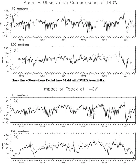
the run without altimetry assimilation are out of phase with the run including altimetry assimilation. During the 1996 season the run without altimetry assimilation completely misses one wave during December. The assimilation of altimetry also helps correct model biases. The zonal cur-rents plotted in Figure 1b very accurately reproduces the strength of the EUC at 140oW as observed by the
[image:11.595.304.559.238.577.2]TOGA-TAO current meter. The zonal current at 120 m from the run without altimetry assimilation (2d) is consistently 20 -40 cm s-1 weaker than the observations.
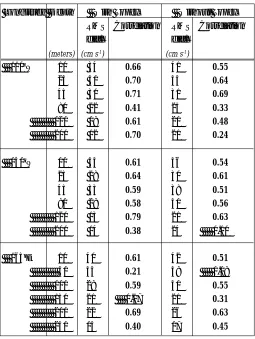
Table I. Statistical comparison of model (with and without Topex assimilation) and observed zonal currents at 110oW, 140oW
and 165oE.
Longitude Depth With Topex Without Topex RMS Correlation RMS Correlation
diff1 diff1
(meters) (cm s-1) (cm s-1)
110oW 10 34 0.66 41 0.55
25 31 0.70 35 0.64
45 30 0.71 31 0.69
80 22 0.41 25 0.33
120 18 0.61 21 0.48
200 12 0.70 21 0.24
140oW 10 33 0.61 36 0.54
25 28 0.64 30 0.61
45 33 0.59 38 0.51
80 29 0.58 31 0.56
120 13 0.79 21 0.63
200 14 0.38 24 0.10
165oE 10 40 0.61 42 0.51
50 34 0.21 39 0.08 100 28 0.59 30 0.55
150 21 0.17 21 0.31
200 22 0.69 26 0.63
250 15 0.40 17 0.45
Correlations in bold are above the 99% significance level.
1Computed after removing the mean from the observations and
the model data.
The statistical analysis presented in Table 1 quanti-fies the contribution of altimetry assimilation at other longitudes and depths. The correlations between the mod-elled currents (with and without TOPEX/Poseidon) and observations are presented. In general, the inclusion of altimetry observations increases the correlation values by about 0.1. The analysis and verification of the model run that includes TOPEX/Poseidon assimilation are covered in detail by Seidel and Giese (1999).
mean climatology from the comprehensive ocean atmos-phere data set (COADS) Dasilva et al., 1994. The model was spun up from 1985 to 1991 using data assimilation of XBT, MBT and TOGA-TAO temperature data. This paper presents the results of two model runs. The first run in-cludes the assimilation of all of the observations listed above. The second run assimilates the temperature obser-vations but does not include the TOPEX/Poseidon altimetry observations.
Verification of Assimilated Currents Against TOGA-TAO Observations
Current meter data are available at several depths from the equatorial TOGA-TAO moorings at 110oW, 140oW
and 165oE. These data are compared to model output from
the run that includes Topex/Poseidon altimetry data to verify model performance. Plots of these comparisons at 10 and 120 m at 140oW are shown in Figures 1a and 1b
(page 12) . For these plots the observed currents have been time averaged over 5 days to match the model output. No manipulation has been performed on the model output. The plot at 10 m (Figure1a) shows the model’s ability to capture zonal current variability over a wide range of time scales. Both the phase and the magnitude of high frequency instability waves agree well with the observations. The sea-sonal variations of the zonal current and of the instability wave energy can be easily identified in these plots. The passage of two equatorial Kelvin waves at 140oW in early
1997 associated with the 1997-1998 El Niño is also clearly visible. The plot of zonal current at 120 m (Figure 1b) dem-onstrates the ability of the model to accurately simulate the Equatorial Undercurrent (EUC) throughout the assimi-lation period except for the first few months of the model run during a period prior to the availability of altimery observations. The model has captured both the mean ve-locity and the variability of the EUC. The shutdown of the EUC associated with the 1997-1998 El Niño is well simu-lated by the model during the first half of 1997. A statisti-cal analysis of all depths for which current meter data is available is presented in Table 1. At 110oW the correlations
(with Topex) range from a high of 0.71 at 45 m to a low of 0.41 at 80 m at 140oW. The highest value at 140oW is 0.79 at
120 m and the lowest value is 0.38 at 200 m. The current meter data available at 110oW covers 63% of the time
pe-riod presented and at 140oW it covers 77%. At 165oE the
current meter data only covers 38% of the time period.
The Contribution of TOPEX/Poseidon
The impact of the TOPEX/Poseidon assimilation at 140o W is presented in Figures 1c and 1d. In these figures
Heavy line - Observations, Dotted line - Model with TOPEX Assimilation
[image:12.595.48.512.82.645.2]Heavy line - Model without TOPEX Assimilation, Dotted line - Model with TOPEX Assimilation
Conclusions
In general, the assimilating model shows good skill in reproducing ocean currents on the equator where moor-ing data are available at 110oW, 140oW and 165oE. The
con-tribution of TOPEX/Poseidon altimetry data is the addi-tion of phase informaaddi-tion in the TIW region and a correc-tion of model biases at depth. Statistically this improves the correlation between model zonal currents and obser-vations by about 0.1. We plan to use a global version of this model coupled with an atmospheric model to investi-gate its value in climate prediction.
References
Carton, J. A., B.S. Giese, X. Cao, and L. Miller, 1996: Impact of altimeter, thermistor, and expendable bathythermograph data on retrospective analyses of the tropical Pacifc Ocean. J. Geophys. Res., 101, 14,147-14,159.
Michael K. Tippett
International Research Institute for Climate Prediction, Palisades, NY, USA
[email protected] Ming Ji
CMB, NCEP, Camp Springs, MD, USA Alexey Kaplan
Lamont-Doherty Earth Observatory of Columbia Uni-versity, Palisades, NY, USA
Introduction
Ocean data assimilation systems combine observa-tions with information from prediction models to produce an analysis or estimate of the ocean state. Statistical inter-polation assimilation methods use observations to correct a model-based first guess and require specification of first-guess and observation error statistics. Often the first-first-guess error covariance (FGEC) is described by an analytical covariance function whose structure is not directly related to ocean dynamics. On the other hand, ensemble and re-duced-space methods represent the FGEC by a low-rank approximation coming from the dynamical model. Here we examine the impact of adding a low-rank FGEC com-ponent to an operational univariate ocean data assimila-tion (ODA) system. Small-scale structures are eliminated from the mean temperature correction and positive impact is seen in the zonal currents.
Ocean data assimilation system
The ODA system uses the MOM-1 Pacific basin model with TAO, XBT and blended SST observations as described in (Behringer et al., 1998). At each assimilation time, the model first-guess is compared to observations and a temperature correction is calculated by minimizing a cost function (Derber and Rosati, 1989). The cost function
re-wards, with weight depending on the observation error covariance, temperature corrections that reduce mismatch between analysis and observations. Simultaneously, tem-perature corrections whose magnitude and spatial struc-ture are incompatible with the FGEC are penalized. The spatial structure of the FGEC controls how first-guess er-rors are corrected in a neighbourhood of the observation, an important property when there are few observations.
Assimilation experiments
We compare a control analysis with one obtained using a FGEC model with low-rank component. The con-trol analysis is produced using a FGEC model Gf with Gaussian horizontal correlations and temperature gradi-ent dependgradi-ent vertical correlations (Behringer et al., 1998). The reduced-space FGEC Sf has the form:
Sf = αGf
⊥ + ZFZT = α(I - ZZT)Gf(I - ZZT) + ZFZT (1)
where 0 ≤ α ≤ 1 is a tunable parameter, the columns of the matrix Z are the EOFs of a simulation and F is a symmetric positive definite matrix. This formulation, like that of Hamill and Snyder (2000) is simple to implement in an ex-isting 3D-Var system; in this formulation however, we as-sume the reduced-space and analytical parts to be uncorrelated. For the special case α= 0 whose results are presented here, calculation of the temperature correction is simplified. We consider the period March, 1993 - Febru-ary, 1997 and use the reduced-space spanned by the first 80 EOFs.
Results
The mean temperature correction and the mean dif-ference between observations and analysis are significantly
Impact of temperature error models in a univariate ocean data assimilation system
da Silva, A. M., C. C. Young, and S. Levitus, 1994: Atlas of Surface Marine Data 1994, Vol. 1, Algorithms and Procedures. Tech. Rep. 6, Natl. Oceanic and Atmos. Admin., Silver Spring, Md.
Kalnay, E., M. Kanamitsu, R. Kistler, W. Collins, D. Deaven, L. Gandin, M. Iredell, S. Saha, G. White, J. Woollen, Y. Zhu, A. Leetma, R. Reynolds, M. Chelliah, W. Ebisuzaki, W. Higgins, J. Janowiak, K.C. Mo, C. Ropelewski, J. Wang, R. Jenne, and D. Joseph, 1996: The NCEP/NCAR 40-year reanalysis project. Bull. Am. Meteor. Soc., 77 , 437-471. Levitus, S., and T. Boyer, 1994: World Ocean Atlas 1994, Vol. 4,
Temperatur. Technical Report No. 4 , U. S. Department of Commerce,Washington, D.C.
Pacanowski, R., 1995: MOM 2 documentation: User's guide and reference manual. Tech. Rep. 3 , Geophys. Fluid Dyn. Lab., Princeton, N.J.
We present an approach for an adjoint method that allows the assimilation of statistical informations into cha-otic ocean models on longer time scales than the predict-ability range. The basic underlying assumption is that a larger predictability exists for planetary scales which are isolated by temporal and spatial averaging. The crucial point of the method is the invention of an adjoint to a sepa-rate prognostic model for the statistical mean used to cal-culate the cost function gradients. Coarse resolution ver-sions of eddy resolving models are applied for this pur-pose. Here we use a 1/3o eddy-permitting forward model
in combination with a 1o backward model. For higher
or-der moments such as sea surface height variance calculated from altimeter data, a closure scheme is required, which is employed by a simple parameterization in analogy to the approach of Green (1970) and Stone (1972). The method is applied for the assimilation of annual SSH variance calcu-lated from TOPEX/POSEIDON and ERS1 in association with climatological data for temperature and salinity from Boyer and Levitus (1997) into an eddy permitting version different from zero, indicating systematic biases (Fig. 1,
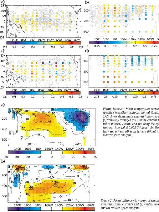
page 17). The reduced-space analysis is generally less con-strained by observations than the control analysis. In both cases, the mean temperature correction is correlated with the mismatch between analysis and TAO data. In the con-trol analysis, the mean temperature correction maxima and minima correspond to TAO locations, producing structures with length-scales on the order of the TAO mooring spac-ing. These structures do not appear in the analysed tem-perature field or its derivatives. In the reduced-space ex-periment, the mean temperature correction attempts to correct the same model and forcing deficiencies but does so with larger scale structures. In both experiments the im-pact on the analysed temperature fields (compared to simu-lation) is qualitatively similar. However, the impacts on the zonal currents are different (Fig. 2, page 17). The mean zonal surface current exceeds -50 cm/sec. in the Eastern Pacific for the control case while the measured value at (0oN,110oW) is -17.3 cm/sec. The equatorial undercurrent
core in the control is weakened by about 12 cm/sec and shifted to the west compared to the reduced-space experi-ment. Similar impacts on zonal velocity are seen when simulations are forced with time-independent mean tem-perature corrections.
Conclusions
Temperature error models in univariate ocean data assimilation systems impact zonal velocity. The tempera-ture corrections produced using a reduced-space FGEC have less small-scale structure and were seen to have a positive impact on zonal currents.
Armin Köhl, Scripps Institution of Oceanography, La Jolla, CA, USA
Jürgen Willebrand, Institut für Meereskunde, Kiel, Germany
Two categories of methods are available for the as-similation of altimeter data. Due to the lack of a precise geoid, application of the sequential method use an addi-tional independent data source for the mean sea surface height since the method is incapable to change the mean state consistent with the assimilated anomalies (The DY-NAMO Group, 1997). The adjoint method searches for an optimal trajectory that by construction represents the data in a dynamically consistent way. The method, however, is due to the use of tangent linear equations in high resolu-tion models useful only on very short time spans of a few months, where the linear approximation holds. Such short periods are not sufficient for a significant transfer of infor-mations into depth.
Variational assimilation of SSH variance from TOPEX/POSEIDON and ERS1 into an eddy-permitting model of the North Atlantic
continued on page 19 In the reduced-space FGEC model used here (α= 0), errors are reduced only on the reduced-space which in the re-duced-space Kalman filter causes divergence (Cohn and Todling, 1996). The choice here of simulation EOFs to span the reduced subspace is not necessarily appropriate even in the most idealized systems since the simulation EOFs do not include the effect of data assimilation or model er-ror (Tippett et al., 2000). Therefore, likely there is benefit in considering a FGEC with both reduced and analytical parts (a>0). Future work will examine impact on forecast skill.
References
Behringer, D. W., M. Ji, and A. Leetmaa, 1998: An improved cou-pled model for ENSO prediction and implications for ocean initialization. Part I: The ocean data assimilation system. J. Climate,126, 1013-1021.
Cohn, S. E., and R. Todling, 1996: Approximate data assimilation schemes for stable and unstable dynamics. J. Meteor. Soc. Japan,74, 63-75.
Derber, J., and A. Rosati, 1989: A global oceanic data assimilation system. J. Phys. Oceanogr.9, 1333-1347.
Hamill, T.M., and C. Snyder, 2000:A hybrid ensemble Kalman filter/ 3D-variational analysis scheme. Mon. Wea. Rev., in press.
100 80 60 40 20 0 20 40 60 80 100
0 50 100 150 200 250 300 350
80 60 40 20 0 20 40 60 80
Longitude
Latitude
Mean Net Heatflux Estimate (W/m2)
100 80 60 40 20 0 20 40 60 80 100
0 50 100 150 200 250 300 350
80 60 40 20 0 20 40 60 80
Longitude
Latitude
Net Heatflux Change (W/m2)
1992 1993 1994 1995 1996 1997 1998
1 0.5 0 0.5 1 1.5 2
W
att
x 1014 VT (g); V‘T‘ (b); V‘T (m); VT‘ (r) 57oN Atlantic
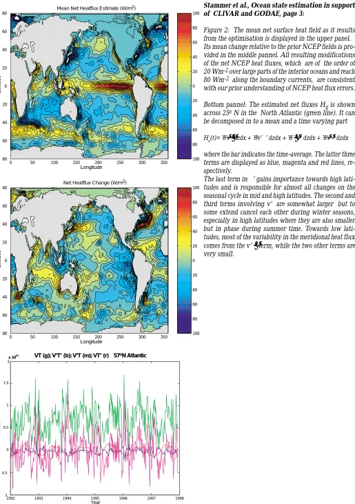
[image:15.595.45.560.62.793.2]Stammer et al., Ocean state estimation in support of CLIVAR and GODAE, page 3:
Figure 2: The mean net surface heat field as it results from the optimisation is displayed in the upper panel. Its mean change relative to the prior NCEP fields is pro-vided in the middle pannel. All resulting modifications of the net NCEP heat fluxes, which are of the order of 20 Wm-2 over large parts of the interior oceans and reach
80 Wm-2 along the boundary currents, are consistent
with our prior understanding of NCEP heat flux errors. Bottom pannel: The estimated net fluxes Hq is shown across 25o N in the North Atlantic (green line). It can
be decomposed in to a mean and a time varying part Hq(t)= ∫∫ v¯θ¯ dzdx + ∫∫ v’θ’ dzdx + ∫∫θ¯ v’ dzdx + ∫∫ v¯θ’ dzdx
where the bar indicates the time-average. The latter three terms are displayed as blue, magenta and red lines, re-spectively.
Figure 1: (a) Instantaneous temperature anomalies at 200 m (01/ 01/89) and corresponding large scale (b) and mesoscale (c) sig-nals (in °C).
Figure 2: (a) Rms of the monthly means of the large scale signal of temperature anomalies at 200 m and (b) rms of mapping error for the three-degree array (in °C).
Guinehut et al., Design of an array of profiling floats in the North Atlantic from Model simulations - preliminary results, page 6:
260.0 270.0 280.0 290.0 300.0 310.0 320.0 330.0 340.0 350.0 0.0 10.0 20.0 20.0
10.0 0.0 10.0 20.0 30.0 40.0 50.0 60.0 70.0
260.0 270.0 280.0 290.0 300.0 310.0 320.0 330.0 340.0 350.0 0.0 10.0 20.0 20.0
10.0 0.0 10.0 20.0 30.0 40.0 50.0 60.0 70.0
260.0 270.0 280.0 290.0 300.0 310.0 320.0 330.0 340.0 350.0 0.0 10.0 20.0 20.0
10.0 0.0 10.0 20.0 30.0 40.0 50.0 60.0 70.0
2.0
1.6
1.2
0.8
0.4
0.0
-0.4
-0.8
-1.2
-1.6
-2.0
260.0 270.0 280.0 290.0 300.0 310.0 320.0 330.0 340.0 350.0 0.0 10.0 20.0 20.0
10.0 0.0 10.0 20.0 30.0 40.0 50.0 60.0 70.0
260.0 270.0 280.0 290.0 300.0 310.0 320.0 330.0 340.0 350.0 0.0 10.0 20.0 20.0
10.0 0.0 10.0 20.0 30.0 40.0 50.0 60.0 70.0
1.0
0.9
0.8
0.7
0.6
0.5
0.4
0.3
0.2
0.1
[image:16.595.247.554.91.455.2] [image:16.595.50.563.91.554.2]40 30 20 10 0 10 20 30 40 140E 160E 180 160W 140W 120W 100W 80W 200 400 600 0 10 10 10 1010 10 10 0 0 0 00 0 0 0 0 0 0 0 0 0 0 0 0 0 0 0
10 10 10
10 10 10 10 10 20 20 20 20 2020 20
3030 30
40 30 20 10 0 10 20 30 40
140E 160E 180 160W 140W 120W 100W 80W 200 400 600 30 20 20 10 10 10 10 10 10 10 10 0 0 0 0 0 0 0 0 0 0 0 0 10 10 10 10 10 10 10 10 10 10 10 10 20 20
Figure 1(above): Mean temperature corrections (positive (negative) contours are red (blue)) and TAO observations minus analysis (colored squares) (a) vertically averaged (50 - 500m; contour inter-val of 0.004oC / hour) and (b) along the equator (contour interval of 0.008oC / hour)) for the con-trol case. (c) and (d) as in (a) and (b) but for the reduced space analysis.
Figure 2: Mean difference in cm/sec of simulation equatorial zonal currents and (a) control analysis and (b) reduced-space analysis.
Tippnett et al., Impact of temperature error models in a univariate ocean data assimilation system, page 13:
1 0.75 0.5 0.25 0 0.25 0.5 0.75 1
140E 160E 180 160W 140W 120W 100W 80W
100
200
300
1 0.75 0.5 0.25 0 0.25 0.5 0.75 1
140E 160E 180 160W 140W 120W 100W 80W
100
200
300
0.8 0.6 0.4 0.2 0 0.2 0.4 0.6 0.8
140E 160E 180 160W 140W 120W 100W 80W
15S 10S 5S 0 5N 10N 15N
0.8 0.6 0.4 0.2 0 0.2 0.4 0.6 0.8
140E 160E 180 160W 140W 120W 100W 80W
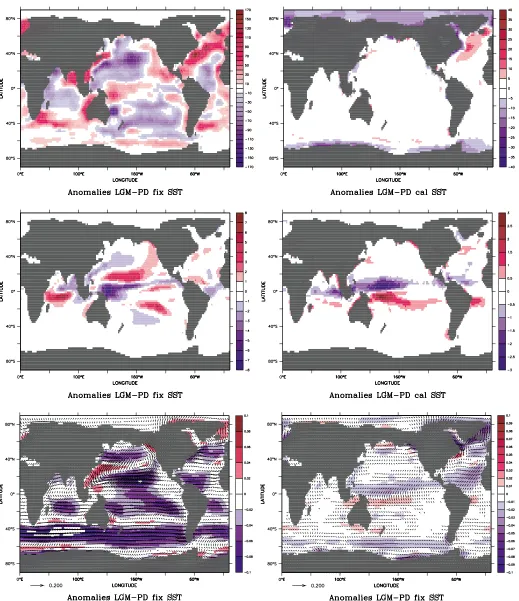
[image:17.595.33.541.89.767.2]Figure 1:
Top: Anomalies of heat flux as mean of 5 models using fixed SSTs (left), and 4 models using calculated SSTs (right).
of the Community Modelling Effort model of the North Atlantic ocean. The intention is to utilize the close corre-spondence between the position of the main frontal struc-tures and the patterns of high variability as demonstrated by Treguier et al. (1997) to estimate the underlying mean state by assimilating variability.
The forward model is described in Oschlies and Willebrand (1996). The horizontal gridspacing is 1/3o in
meridional and 2/5o in zonal direction. It is forced with
monthly mean wind stresses of Hellerman and Rosenstein (1983) and the heat flux is formulated according to the lin-ear approximation of Han (1984). Surface fluxes of fresh water are specified by relaxating salinity to the monthly mean values of Levitus (1982). The adjoint is constructed from the modified code of the 1 degree version with aid of the automatic adjoint code compiler TAMC developed by Giering and Kaminski (1998). Initial conditions for tem-perature and salinity are estimated and mean values of the subsequent year are analysed.
The effect of the parameterization which is based on baroclinic instability theory is to suggest steeper frontal structures at locations where the 1/3o model
underesti-mates variability in proportion to the observations. The lo-cations of the Azores front and the Gulf Stream are clearly visible in the cost function gradient from the first iteration displayed in Figure 1 . The gradient results from the SSH-variance data term alone and it is directly related to the proposed changes of the temperature initial condition. Spatial gradients visible in Figure 1 thus correspond to spatial gradients in the change of the temperature field.
It is found that SSH variance data can introduce com-plementary informations about the main frontal structures
consistent with climatologies since sharp fronts are usu-ally appear too smooth in climatological data. Figure 2 (page 20) demonstrates the close linkage between mean SSH and its variability. The mean front of the control as visible from mean SSH and the associated variability is displaced northward and too weak. The mean SSH is cor-rected after optimization to almost the same position and strength visible in the data from Singh and Kelly (1997), although the northward turn of the North Atlantic Currrent at 42oW is not captured. According to the physical basis
implemented within the closure scheme baroclinic insta-bility is enhanced in connection with the strengthening of the frontal structures. The level of variability is increased to the observed, although the pattern extends slightly fur-ther to the north around 55oW and misses the extension at
40oW. Eddy scales remain too large due to still too low
reso-lution.
The resulting annual mean state, though not fully consistent with the assimilated data, is markedly improved in comparison with the reference state. Not surprisingly, after a few years of forward integration without assimila-tion the state will however return back to the first guess state.
Acknowledgements
The work was supported by the German WOCE through the BMBF under contract number 03 F 0157 A.
References
Boyer, T. P., and S. Levitus, 1997: Objective analyses of tempera-ture and salinity for the world oceanon a 1/4degree grid. NOAA Atlas NESDIS 11, U.S. Gov. Printing Office, Wash-ington, D.C.
Giering, R., and T. Kaminski, 1998: Recipes for Adjoint Code Con-struction. ACM Trans. on Math. Software, 24, 437-474. Green, J. S. A., 1970: Transfer properties of the large-scale eddies
and the general circulation of the atmosphere. Q. J. R. Me-teor. Soc., 96, 157-417.
Han, Y.-J., 1984: A numerical world ocean general circulation model part II. a baroclinic experiment. Dyn. Atmos. & Oceanogr., 8, 141-172.
Hellerman, S., and M. Rosenstein, 1983: Normal monthly windstress over the world ocean with error estimates. J. Phys. Oceanogr., 13, 1093-1104.
Levitus, S., 1982: Climatological atlas of the world ocean. NOAA Tech. Paper, 173 pp.
Oschlies, A., and J. Willebrand, 1996: Assimilation of Geosat al-timeter data into an eddy-resolving primitive equation model of the North Atlantic Ocean. J. Geophys. Res., 101, 14,175-14,190.
Singh, S., and K. A. Kelly, 1997: Monthly maps of sea surface hight in the North Atlantic and zonal indices for the Gulf Stream using TOPEX/Poseidon altimeter data. Woods Hole Ocea-nographic Institution Technical Report, WHOI-97-06, 50pp. Stone, P. H., 1972: A simplied radiative-dynamical model for the
[image:19.595.37.291.513.720.2]static stability of rotating atmospheres. J. Atmos. Sci., 29, 405-418.
Fig. 1: Horizontal section through the gradient of the cost func-tion part JSSH with respect to the temperature initial condifunc-tion. The cost function part JSSH measures the difference of the SSH variances between observed and simulated, ci=0.1oC-1; dashed lines negative.
The DYNAMO Group, 1997: DYNAMO Dynamics of North At-lantic Models: Simulation and assimilation with high reso-lution models, Berichte aus dem IFM Kiel Nr. 294.
Mike K. Davey, Matt Huddleston
The Met. Office, London Road, Bracknell, UK [email protected]
Ken R. Sperber
PCMDI, Lawrence Livermore National Laboratory, Livermore, CA, USA, and the model data contributors.
The tropics are regions of strong ocean-atmosphere interaction on seasonal and interannual timescales, so a good representation of observed tropical behaviour is a prime objective for coupled ocean-atmosphere models. As previous assessments focusing on the tropical Pacific have established (Mechoso et al., 1995, Neelin et al., 1992), it has been difficult to develop coupled general circulation models (CGCMs) with the right balance of oceanic and at-mospheric processes and interactions in the tropics. Sys-tematic errors in sea surface temperature (SST) were often largest in the equatorial Pacific, and model representations of El Niño Southern Oscillation (ENSO) variability were often weak and/or incorrectly located.
To broaden and update the previous assessments, two companion projects were initiated by the CLIVAR Nu-merical Experimentation Group 1 (NEG1): the El Niño Simulation Intercomparison Project (ENSIP, organised by Mojib Latif) and the Study of Tropical Oceans In CGCMs (STOIC). (NEG1 subsequently evolved into the CLIVAR Working Group on Seasonal to Interannual Prediction, WGSIP) Monthly SST, surface wind stress and upper ocean vertically averaged temperature (VAT) data from 24 cou-pled models were collected, along with observational analyses. From the submitted data, annual means, annual cycles and interannual anomalies were calculated for 20-year samples. Of the participating models, 22 are coupled GCMs, of which 14 use no form of flux adjustment in the tropics. The models vary widely in design, components and purpose. Note that the model data were submitted in 1997 and 1998, so the results do not necessarily indicate the per-formance of current versions. Many of the models have also been assessed collectively as part of the Coupled Model Intercomparison Project (CMIP). Model ENSO behaviour from an atmospheric viewpoint has been described by AchutaRao et al. (2000).
The aim was to compare the various models against observations, to identify common weaknesses and strengths and to provide benchmarks for future models. Results from ENSIP, concentrating on the equatorial Pa-cific, have been described by Latif et al. (2000), denoted ENSIP2000 henceforth. The STOIC analyses extend beyond the equatorial Pacific, to examine behaviour in all three tropical ocean regions (Atlantic, Indian and Pacific), includ-ing inter-ocean relationships. A detailed report on STOIC
has been completed, and is available via anonymous ftp at ftp://email.meto.gov.uk/pub/cr/ in the gzipped files mkdavey_stoic_doc.gz (text as Word document) and mhuddleston_stoic_figs_050700_tar.gz (postscript figures). Some of the main annual and interannual features found in the comparisons between models and observations are summarised below. For observations we have used the GISST3 SST dataset from The Met. Office, wind stress from WM-COADS and Southampton Oceanography Centre, and upper ocean temperature from Scripps Institution of Ocea-nography.
Annual mean SST
The equatorial section for CGCMs with no tropical ‘flux adjustment’ is shown in Fig. 1 (page 1). The labels indicate the various models: for details see the detailed re-port or ENSIP2000. (Note: the PAC and ATL sub-labels denote separate submitted datasets. However, only UCLA PAC and UCLA ATL are actually different CGCMs.) In most of the Pacific sector, described in detail in ENSIP2000, it is evident that most models have SST too cool by 2 to 3oC,
but the strong central equatorial Pacific east-west SST gra-dient is by and large correct. Several have substantial warm biases in the east Pacific approaching the South American coast. In the equatorial Atlantic nearly all models have the wrong east-west gradient, with SST commonly too cool in the west and too warm in the east. In the Indian ocean sec-tor most models simulate the SST gradient quite well, of-ten with a cold bias. From meridional SST sections it is also evident that most have a too-prominent equatorial cold trough in the east Pacific and central Atlantic.
Among the 8 CGCMs with ‘flux adjustment’ (not shown), all but one has SST within +/- 1oC of observations
over most of the equatorial region.
Annual mean zonal wind stress
Several common features were evident over the equatorial oceans: the majority of the models have mean easterlies that were too weak in the equatorial Atlantic, and westerlies too weak (easterly in several cases) in the In-dian sector. Among CGCMs with no ‘flux adjustment’, most have easterly wind stress too weak in the central equato-rial Pacific but easterly wind stress too strong in the west equatorial Pacific. Among CGCMs with ‘flux adjustment’ mean zonal wind stresses were generally close to observed values in the equatorial Pacific, with largest differences in the central Pacific, but were often too weak in the Indian and Atlantic sectors.
With regard to the Pacific, the mean equatorial SST errors are quite similar to those found in previous CGCM Treguier, A. M., I. Held, and V. Larichev, 1997: Parametrization of quasigeostrophic eddies in primitive equation ocean mod-els, J. Phys. Oceanogr., 27, 567-580.
comparisons. The wind stress errors are also similar, with too-weak (too-strong) central (west) Pacific easterly wind stress accompanying too-cold SST in most of the ‘no-ad-justment’ group. There is also still a tendency for the cold tongue to be too narrow and too strong. As many of the OGCMs use basically the same mixing and advection schemes as in the Mechoso et al. (1995) CGCM sample, it seems likely that errors in representing upper ocean equa-torial mixing and circulation (compounded by ocean-at-mosphere interaction and feedbacks) lead to these equato-rial biases. The warm bias in the east equatoequato-rial Pacific SST is also common to previous CGCM assessments, and here it is also evident in the Atlantic. This is often associated with reductions in stratus cloud in those regions in CGCMs.
Interannual variability
In the equatorial central-east Pacific most models (both with and without flux adjustment) substantially un-derestimated the observed SST variability levels, while many had excess variability in the west Pacific. This was a symptom of a tendency to misplace maximum variability too far west. The majority of models also underestimated SST variability in the Atlantic sector, but matched observed levels in the Indian ocean. With regard to zonal wind stress, most models also substantially underestimated central equatorial Pacific variability, many underestimated vari-ability in the Indian region, but most were comparable to observed levels in the Atlantic sector.
The Pacific results are illustrated in Fig. 2 by a scatterplot of SST standard deviations in the Niño-3 region (5oN-5oS,
150oW-90oW)) against zonal wind stress standard
devia-tion in a central equatorial Pacific region (5oN-5oS,165o
E-225oE). Although allowance must be made for the effect of
the limited sample sizes, regions selected, and multi-decadal fluctuations in activity, is is evident that few of the models approach observed levels of interannual variabil-ity. As expected in a region of strong ocean-atmosphere coupling, wind stress variability tends to increase with SST variability. The lack of model wind stress variability is of-ten more severe than the shortfall in SST variability.
With regard to interannual variability, the ‘no-ad-justment’ group tended to perform better than the ‘ad-justed’ group. Part of the explanation for this difference is likely to be that the ‘no-adjustment’ models generally had higher resolution than the ‘adjusted’ models, particularly in the near-equatorial ocean regions. Note also that simu-lation of tropical variability was not a primary aim for sev-eral of the models.
Interannual correlations between SST’ and Niño-3 SST’
Observations reveal a distinctive horseshoe pattern of negative correlations in the tropical Pacific, but only a few models could reproduce this feature. Most incorrectly had positive correlations in the west equatorial Pacific, which is largely a consequence of having the maximum
0.0 0.5 1.0 1.5 2.0
Std. Dev. of NINO3 SST anomalies 0.000
0.005 0.010 0.015 0.020 0.025
Std. Dev. of central Pacific region zonal windstress anomalies
X Z
A
a
B
C
D b
c d
e E
F G
H
g
I
J h
K
L i
M
X) SOC vs GISST Z) COADS vs GISST A) BMRC
a) CCC B) CCSR C) CERFACS D) COLA PAC b) DKRZ OPYC c) DKRZ LSG d) GFDL R15 e) GFDL R30 E) IPSL TOGA
F) IPSL HR G) IPSL LR H) JMA g) LAMONT I) METO CM3 J) MPI h) MRI
K) NCAR CSM PAC L) NCAR WM PAC i) NCEP
[image:22.595.61.536.414.751.2]M) UCLA PAC