Finite element optimizations for efficient non linear electrical tomography reconstruction

Finite Element Optimizations for Efficient

Non-Linear Electrical Tomography Reconstruction

M Molinari, H Fangohr, J Generowicz, SJ Cox

Department of Electronics and Computer Science University of Southampton, SO17 1BJ, UK

[email protected]

ABSTRACT

Electrical Tomography can produce accurate results only if the underlying 2D or 3D volume discretization is chosen suitably for the applied numerical algorithm. We give general indications where and how to optimize a finite element discretization of a volume under investigation to enable efficient computation of potential distributions and the reconstruction of materials. For this, we present an error estimator and material-gradient indicator as a driver for adaptive mesh refinement and show how finite element mesh properties affect the efficiency and accuracy of the solutions.

Keywords 2D/3D Finite Element Method, mesh quality, adaptive meshing, optimal finite element

meshes, 3D visualisation

1

INTRODUCTION

Electrical Tomography (ET) is an imaging method which tries to reconstruct differing electrical properties of materials within a volume given only surface potential measurements resulting from an injected current. It is a non-invasive and cost-effective imaging technique based on an iterative computational algorithm which solves a non-linear least-squares minimization problem.

ET reconstruction procedures can only produce accurate results if the discretization of the volume under investigation is chosen suitably for the applied numerical algorithm. Often, a poor discretization yields inaccurate results since it affects several steps of the reconstruction process (forward solution, inverse problem, final visualisation).

Current ET algorithms employ increasingly the Finite Element (FE) method to obtain a discretization which is flexible enough to represent arbitrary geometries, robust and simple in terms of numerical handling and established and well known in many areas of engineering technology (Silvester and Ferrari, 1996, and Salazar-Palmaet al., 1998). Furthermore, the FE representation of a domain allows for easy application of different types of boundary conditions and effective handling of local refinement – an important requirement for efficient reconstruction.

One important problem in 2D and 3D Electrical Tomography is therefore the ability to generate quality FE meshes for arbitrary geometries. In particular medical applications have very demanding requirements in terms of object shapes where the human head or torso geometry are much more difficult to represent with FE models than symmetric pipe or vessel structures used in industrial processes. Moreover, in medicine we have to deal with individual patients so that methods are required which easily modify/reshape pre-defined template meshes to fit the individual’s geometry and/or internal structure.

Our aim is to allow not only for an accurate but also for a fast reconstruction. This leads to a balancing decision between accuracy and speed. However, if certain optimizations are applied to the Finite Element mesh, accuracy does not have to be an impediment to fast reconstruction.

Finally, we will present some results of forward solutions and reconstructions in section 3 before drawing our conclusions in section 5.

2 THE FINITE ELEMENT METHOD FOR ELECTRICAL TOMOGRAPHY

The reconstruction algorithm in Electrical Resistance Tomography computes the conductivity distri-butionσ(r) which minimises the squared error between voltage measurements U0and their computed counterpartsU(σ), both on the surface of the domainΩ.

The electric field in the volume conductor Ω is governed by the Poisson equation together with Dirichlet and von Neumann boundary conditions:

(

(

)

∇

(

)

)

=

0

⋅

∇

σ

r

ÿ

u

r

ÿ

0

)

(

r

U

u

ÿ

=

n

j

n

r

u

r

=

∂

∂

ÿ

ÿ

ÿ

(

)

)

(

σ

whereσ(r) represents the conductivity at position r, and u is the potential distribution inΩ.U0denotes the measured voltages at the boundary electrodesδΩVEL, andn denotes the outward normal across the current injection electrodes δΩCEL where a current of normal density jn is injected. The set of boundary conditions can differ if specific electrode models are used, for example the Complete Electrode Model for which Somersaloet al. (1992) have shown uniqueness and a modelling error of 0.1% of the experimental measurements.

The reconstruction algorithm makes intensive use of the solution of the forward problem, which is the computation of an approximate potential distributionuh(r) on the volumeΩ given injected currents I and an assumed conductivity distributionσ(r). By applying a discretization method to the domain, the differential equation (1) is transformed into a linear system of equations:

N

N

I

U

Y

(

σ

)

=

whereY is the conductivity dependent admittance matrix of size NxN, UNa vector containing the nodal voltages and IN a vector describing the injected currents. The size of Y, UN and IN depends on the number of nodes, N, which is determined by the type of element and the order of the employed interpolation function for the approximationuhofu:

ÿ

=

r

U

u

)

(

ÿ

ϕ

where theUi are the nodal voltages and theϕi represent basis or shape functions for the solution, sometimes also called interpolation functions (Burnett, 1987).

For the discretization of the area or volume under investigation, the Finite Element Method (FEM) has many advantages over other methods. Boundary conditions are easier to apply than for the Finite Difference Method (FDM), which gives only pointwise approximations compared with piecewise approximation of the solution in FEM. It is also less straightforward to locally refine a finite difference mesh around a region of interest. The Boundary Element Method (BEM) is usually applicable only for cases where there are few regions with differing conductivities inΩ. (Webster, 1990)

2.1 Mesh Quality

• element geometry and quality

• element and node density

• boundary representation of domain

• beneficial enumeration of topology and nodes

• order and type of basis functions

Many of the meshing programs available in the public domain often do not fulfil all of the requirements laid down by the first four items listed. The fifth factor, the use of appropriate interpolation functions on the discretization, is more a choice of the reconstruction software user. This however is restricted by the available computational resources and time to be spent. With an appropriate enumeration of the nodes in the mesh, the matrix operations involved become more efficient. We will have a more detailed look at some of these factors:

Element Geometry & Quality. Whilst for applications such as viscous fluid flow simulations elements

with high aspect ratios are wanted, general problems with lower variations in flux, such as for example ET, require elements with more regular shape. In 2D, the use of equilateral triangles and in 3D the use of regular tetrahedrons allows the discretization of a domain without preferring any particular direction. This property is known as geometric isotropy (Burnett, 1987) and ensures that one variable is not represented more accurately than the others.

A limited set of possible measures for the quality of elements, which are equally applicable to 2D and 3D, is given here:

3 1 1 surface ideal surface true volume ideal volume true ≤ ≤ + +

= q_gm

gm q (6) 1 0 3 / 1 volume sphere volume true 3 2 9 ≤ ≤ = rr q rr

q π (7)

1 0

D ≤ ≤

= q o R i R q (8)

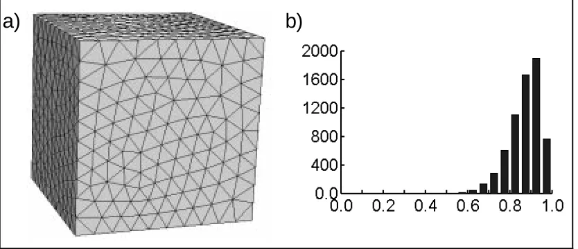
qgmandqrrare presented and discussed in Robertet al. (1998) in the context of optimising tetrahedral space station arrangements. The higher the value, the better the quality of the element. We will employ the quality measureq presented by Golias and Dutton (1997). RiandRodenote the radius of inscribed and circumscribed circle/sphere respectively andD is the dimension of the problem. Figure 1(b) shows a typical quality distribution of q on the 3D mesh in figure 1(a). From the bar graph distribution, we can visually determine how good the overall mesh quality is. As quantitative parameters for the quality, we will use the mean value of theq-distribution and its standard deviation.

a)

b)

Element and Node Density. By applying the Finite Element Method, we convert the continuous

problem into a problem with a finite number of unknowns. It is known that as the element size decreases to zero, the solution on the discretization tends to the true solution (Burnett, 1987). Too large a number of elements and nodes makes a reconstruction impractical. An appropriate balance must be struck between accuracy of solution and the time/memory used in obtaining it.

Often a fine discretization of the domain is not necessary as additional nodes/elements do not lead to increased accuracy in particular cases or regions. It is possible to generate meshes with elements whose sizes vary with position according to a desired density distribution. This density distribution should either be pre-defined by the user (with information from other sources, for example Computer Tomography images) or should be computed by the software during the course of the reconstruction (see later discussion on mesh construction and refinement).

Boundary representation. A good discretization will follow the boundary representation as accurately

as possible. Nurbs and Splines are preferable boundary definitions as these represent the boundary using higher order polynomials, however, often a surface can only be described by point definitions.

It is possible to use isotropic Finite Elements which deform to match the boundary with quadratic interpolation, however, numerical analysis showed (Szabo, 1986) that this can sometimes introduce additional errors instead of avoiding them. Sometimes it is desirable to use so-calledinfinite elements to model openings of volumes, such as the throat in human head volumes or a section of a pipe.

The geometric accuracy of the boundary definition not only affects the accuracy of solution but can also introduce artefacts from wrong electrode representations which affect the accuracy of the boundary conditions. In the case of ET, this will have major negative effects, as the main current density source will not be represented correctly.

Jainet al. (1997) showed that the error in reconstruction of a volume can reach 37% if a circularly shaped boundary is assumed instead of a correct elliptical boundary with axis ratio 0.64.

Order of basis interpolation functions. Not only the shape but also the order of the basis functions

on the elements plays an important role in the accurate representation of the solution on the mesh. The shape functions in equation (5) can be standard polynomials or – depending on the symmetry of the domain – Bessel or Legendre functions or any other type of C0functions. It is desirable to use a problem-adapted base function which simplifies the numerical approximation and provides a high level of accuracy.

The most suitable shape functions for arbitrary geometries are Lagrange interpolation polynomials. They provide interpolation up to any desired polynomial order. We note that with increasing order (so-calledp-refinement), the number of interpolation nodes required for a given mesh increases and the subsequent higher computational cost leads to an increase in computation time. We can see from the work of Vauhkonenet al. (1999) that for achieving a better accuracy of a factor 2 to 5, the number of interpolation nodes in the p-refinement case increases by a factor of 7, which leads to a slow-down of at least a factor 10 in the reconstruction.

We have decided to employ simple piecewise linear shape functions which are both fast to compute and easy to maintain in programming structures. The computing time saved in this way is then spent on refining the mesh locally rather than assuming global higher-order functions.

2.2 Mesh Generation & Refinement

Good mesh generators should be able to meet the following criteria:

User Input

• ability to accurately define boundaries

• possibility to specify a node or element density function

• allowing for remeshing of existing meshes

Meshing

• create unstructured mesh to avoid anisotropies

• create elements with high quality

• generate element density according to user input

• perform automatic computation without requirement of user interaction

• carry out fast construction of meshes

• being robust: creation of valid meshes

Output

• restricted to useful and meaningful parameters, such as topology and node positions

• possibility of choosing different output structures (topology, edge connection, etc.)

The Handbook of Grid Generation (Thompson et al., 1999) and the Meshing Research Corner (http://www.andrew.cmu.edu/user/sowen/mesh.html) present and discuss many different methods for the generation of finite element meshes. However, it seems that many researchers do make use of meshing programs without considering the impact of unsuitable volume discretizations on the reconstruction.

We have found that mesh generation based on physical principles gives best results in terms of element shape and grading. In particular, we have employed two novel methods of generating high quality meshes fitted to a given mesh density: (a) a modified version of bubble meshing (Cingoskiet al. 1997) and (b) a vortex dynamics (Fangohr et al., 2000, 2001) meshing technique. Both methods are based on Molecular Dynamics (MD) principles (Haile, 1997) which minimize the system’s energy:

(a) In modified bubble meshing, the nodes of the mesh are represented by spheres of finite size, interacting only with their nearest neighbours according to Hooke’s law. The variation of the node density across the domain results from making the radius of the bubbles a function of their position.

(b) In vortex meshing, repulsive forces govern the equations of motion of the point-like vortices which have no spatial extension. An additional potential distribution enforces the density variation of nodes in the mesh.

The theoretical ground state (i.e. the lowest energy configuration) of both methods in the absence of density variations is in two dimensions a hexagonal lattice and generally the closest sphere packing configuration (Aste and Weaire, 2000). For bubble meshing, this configuration corresponds to the lattice of atoms in solid state matter, whereas for vortex meshing it relates to the (two-dimensional) Abrikosov state (for a review see Blatteret al., 1994) in Type-II Superconductors.

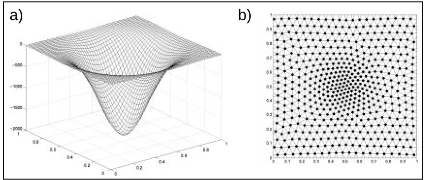
a)

b)

Figure 2: (a) ‘Pinning’ potential used for the vortex dynamics meshing method resulting in (b) high quality 2D mesh with continuous change in density.

potential (it reduces their energy) and thus vortices accumulate in the centre of the domain. Figure 3 shows a corresponding result from the bubble meshing technique.

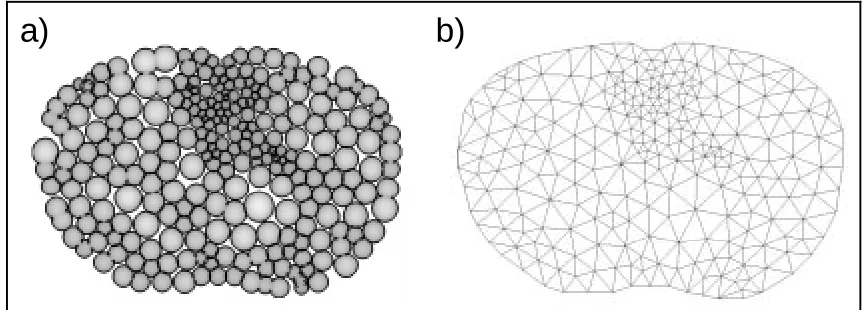
b)

a)

Figure 3: (a) ‘Bubbles’ moving to form an optimal configuration and (b) the triangulated positions of the centres of the bubbles give a finite element mesh with well-defined characteristics.

Meshing algorithms usually employ the Delaunay triangulation method for which fast and hence efficient algorithms exist, for example the qhull package (Barberet al., 1996). Table 1 gives an over-view of some meshing methods and their performance benefits.

Method 2D 3D density quality remeshing time

Advancing

front ÿ ÿ adaptive good no fast

Bubble

Meshing ÿ ÿ adaptive high yes

fast – moderate Vortex

Dynamics ÿ ÿ adaptive very high yes moderate

Mesh conforming

refinement ÿ

– dependent on

previous mesh

dependent on

previous mesh yes very fast

Table 1: Properties of different Finite Element mesh creation techniques.

Mesh refinement

We have shown that adaptive mesh refinement is a highly applicable technique for 2D Electrical Impedance Tomography (Molinariet al., 2001). An initial coarse mesh can be refined to improve the accuracy of the solution as well as the resolution of material boundaries. The local refinement is then based on error or material gradient indicators, which guide the refinement process in regions of interest or where the solution varies rapidly. This saves a large amount of computation time for obtaining results of same accuracy compared to globally fine meshes.

Three major methods of mesh refinement are presented in literature. These include

• h-refinement, where the elements are subdivided into smaller ones

• p-refinement, which uses higher order interpolation functions for the solution

• r-refinement, which relocates the existing nodes in a mesh

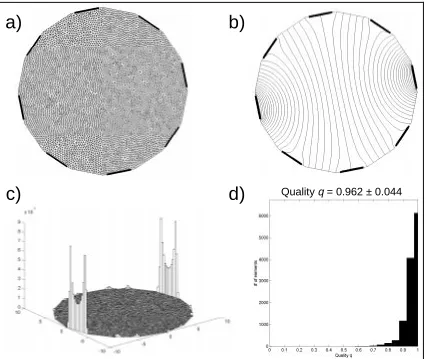
Qualityq = 0.962 ± 0.044

b)

a)

d)

c)

Figure 4: (a) The finite element mesh consisting of 6047 nodes and 11890 elements used for the most accurate computation of the potential shown in (b). The error estimator indicates that the error of the solution is large at the edges of the electrodes, especially of the two current injection electrodes (c). Graph (d) shows the very

high geometrical quality of the elements in the mesh.

2.3 Error Estimation

Since the true solution for the problem is unknown (otherwise we would not have to compute it numerically), the error of the approximation on the discretization is unknown. However, once an approximated solution of the potentials at the nodes of our mesh is obtained, we can calculate a so-calleda posteriori error estimate on an element and the mesh (Salazar-Palma 1998, Bathe 1982). In Electrical Tomography, the solution of the forward problem gives us the potential at the nodes of our mesh with linear interpolation. The normal component of the current density within each element has to be continuous across interelement boundaries. The approximate solution obtained from the FE discretization usually violates this (smoothness) condition. We can estimate the square norm of the error of the forward solution on elemente,Σf

2

(e), by summing the jumps of the squared residuals of the current density normal components (σ∇∇∇∇u) across the surfaces between element e and its f th neighbour, given by the outward normal vectorsef.

(

)

ÿ

∇

−

∇

⋅

=

Σ

f

ef f f e e

f

e

g

r

u

u

s

1

2 2

)

,

(

)

(

ÿ

σ

σ

σ

ÿ

g(r,σ) is a geometrical factor, taking into account the positions of the nodes, r, and the element’s conductivityσ. To obtain the total error on the mesh, we sum up the contributions of each element and take its norm

ÿ

Σ

=

Σ

elements all

2 ,total f

(e

)

This error estimate is both, physically sound and robust (Salazar-Palma, 1998) and can be carried out quite quickly. Again, for higher order elements, more terms have to be taken into account and integrals across the element’s surface and in its interior have to be determined, which can slow down the computation significantly.

Applying this error estimate to an object with surface electrodes attached, we observe that the largest error is located in regions with highest current density, which is around the electrodes. This error in boundary regions around the electrodes affects the solution in inner regions of the domain significantly so that refinement is desirable as presented above.

Another possibility of mesh refinement is based not on the error but on the gradient of conductivity between neighbouring elements. This results in higher resolution of material boundaries, which allows for better image resolution in ET. The material gradient estimator used in the inverse problem Σi is computed using the distance of the centres of mass of the elemente and its neighbour f, and their respective conductivities,σeandσf:

ÿ

−

=

Σ

f ef

f e i

d

e

1

)

(

σ

σ

2.4 Mesh Templating & Deformation

In medical applications such as functional brain imaging, there arises the need for meshes which have certain built in features, for example a local high mesh density around the optic nerve or pre-defined materials in local regions. For this purpose, mesh templates can be defined which consist of a mesh corresponding to an ‘average’ model of the domain, for example the head. Methods are required to easily modify/deform this pre-defined template mesh to fit individual patients’ geometries and/or internal material structures. Powerful tools exist for this type of reshaping, however, it would be useful to have Electrical Tomography software packages which incorporate this possibility.

Our meshing methods allow for the reshaping of existing meshes by changing the bubble size in bubble meshing or the potential in the vortex dynamics based technique. Hence no new mesh needs to be computed and optimized mesh templates can be re-applied to many topologically equivalent shapes.

2.5 Node Renumbering / Parallel Optimization

The solution of the linear system of equations (4) is usually performed by an iterative method, it is therefore desirable to renumber the nodes in the mesh to obtain a matrix for which the iterative process will converge quickly. Standard methods for node renumbering exist and can be found in Pissanetzky (1984). We have also demonstrated that it is possible to obtain the solution of the linear system (4) using a cluster of computers working in parallel (Blottet al., 2000). This can allow for real-time reconstruction for continuous monitoring of a patient.

2.6 Visualisation

The results of tomographic reconstruction are often difficult to visualise in a way useful for clinicians/human monitors. In particular, the three-dimensional visualization is not very simple in the coding/programming sense.

The FE meshes used for reconstruction can also be used for visualisation. By applying clipping planes or isosurface display techniques, quantities such as potential, current density, material, etc. in the interior of a volume can efficiently be presented to the user.

3 RESULTS

We show Electrical Tomography reconstructions of the same configuration on different types of 2D Finite Element meshes. All meshes are based on first order linear interpolation functions with constant conductivity values across the elements. The quality of the mesh can be given as a bargraph or – as we applied it – as a mean value of the distribution and its standard deviation. The following table gives a quantitative overview of the different meshes used.

# Nodes # Elements Quality Q Error E Time (ms)

17 16 0.63 0.40 10

27 36 0.92 0.24 10

43 68 0.96 0.21 14

56 91 0.95 0.19 20

77 121 0.93 0.17 30

136 233 0.95 0.14 50

267 472 0.94 0.12 100

511 947 0.96 0.09 230

823 1542 0.95 0.07 441

2447 4727 0.96 0.01 3560

6047 11890 0.96 (0.00) ~19 sec

Table 2: Different timings for meshes on which the solution of the forward problem in ET was computed. Please find the explanation for the variables in the text.

136n, 233e E = 0.14 17n, 16e E = 0.40

2447n, 4727e E = 0.01 267n, 738e

E = 0.12 43n, 68e E = 0.21

77n,121e E = 0.17

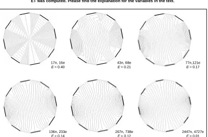
Figure 5: Potential distribution for differing finite element meshes. The numbers next to the meshes indicate the number of nodes and elements used.Edenotes the error of the solution on the mesh.

memory allocation and assembly of the system matrix, computation of the matrices relevant for the complete electrode model (CEM), assembly of the CEM system matrix and finally the solution of the system given in (4). The time was taken on an AMD Athlon Processor running at 500 MHz and using MATLAB as a prototyping software package. To obtain an accurate estimate of the ‘true’ solution we computed the voltages at the electrodesUmeasusing the mesh with 11890 elements and used these in the calculation ofE.

We can see that the element density is the most critical component in terms of accuracy. In figure 5, we present the variation in the potential distribution for an identical current injection all cases, coming in at three o’clock through the electrode indicated by the bar around the boundary and coming out at the opposite electrode, positioned at nine o’clock.

By making the mesh denser or improving the quality we can see that forward solution and resolution improve by a factor of approximately 2 for employing ten times as many elements/nodes resulting in ten times the computation speed.

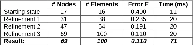
Table 3 contains the refinement steps carried out on the initially very coarse and unsuitable mesh with 17 nodes and 16 elements. Figure 6 shows the improvement of accuracy in the forward solution by using adaptive, error-estimator based refinement. Comparing the time (81 ms) and error (0.110) to the values given above, we achieved a result equivalent to the use of a mesh of size 267 nodes or 472 elements respectively.

# Nodes # Elements Error E Time (ms)

Starting state 17 16 0.400 11

Refinement 1 31 38 0.235 20

Refinement 2 47 64 0.191 20

Refinement 3 69 100 0.110 20

Result: 69 100 0.110 71

Table 3: Auto-adaptive refinement decreases the error on the solution using less nodes / elements than the ‘standard’ case and even in less time!

4 CONCLUSIONS

We have addressed important issues of the reconstruction process in Electrical Tomography Imaging. The underlying finite element discretization affects the results to a great extend and certain optimizations such asoptimal meshing at the start of the imaging process as well as adaptive meshing during the course of the reconstruction process are highly desirable.

Results show that even for simple 2D meshes, a significant improvement in performance can be achieved without much effort if the discussed optimizations are employed. We believe that this work contributes to the realisation of fully non-linear real-time imaging or patient monitoring in hospitals. Further work will incorporate most of the techniques presented here in a parallel non-linear solver to enable fast and accurate electrical impedance reconstructions for medical and industrial application.

5 REFERENCES

Aste T, Weaire D, (2000),The pursuit of perfect packing, IOP Publishing, Bristol, UK

Barber CB, Dobkin DP, and Huhdanpaa H, (1996), The Quickhull Algorithm for Convex Hulls, ACM Transactions on Mathematical Software 22, pp. 469-483

Bathe KJ, (1982),Finite Element Procedures in Engineering Analysis, Prentice Hall Inc, USA

Blatter G, Feigel’man MV, Geshkenbein VB, Larkin AI, and Vinokur V, (1994), Vortices in high-temperature superconductors.Rev Mod Phys 66, pp. 1125-1388

b)

a)

d)

c)

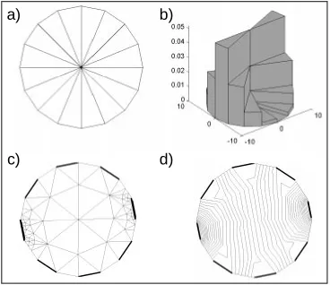
Figure 6: (a) shows an unsuitable mesh for reconstruction which we will refine according to the error estimator on the elements shown in (b). After three auto-adaptive refinement and smoothing steps, we obtain the mesh in (c) which results in the potential distribution in (d). This adaptive meshing is much faster and produces more accurate results

than global fine meshes (see table 3).

Burnett DS, (1987),Finite element analysis, from concepts to applications, Addison-Wesley.

ÿingoski V, Murakawa R, Kaneda K, Yamashita H (1997). Automatic Mesh generation in finite element analysis using dynamic bubble system.J. Appl. Phys. 81(8), pp.4085-7.

Fangohr H, de Groot PAJ, and Cox SJ, (2001), Critical Transverse Forces in Weakly Pinned Driven Vortex Systems,Physical Review B, 63, pp.1-5

Fangohr H, Price AR, Cox SJ, DeGroot PAJ, Daniell GJ, Thomas KS (2000). Efficient Methods for handling Long-Range forces in Particle-Particle Simulations.J Comp Phys, 162, pp. 372-384

Golias N A and Dutton R W, (1997), Delaunay triangulation and 3D adaptive mesh generation,Finite Elements in Analysis and Design 25, pp. 331-341

Haile JM, (1997),Molecular Dynamics Simulation, Elementary Methods, John Wiley & Sons

Jain H, Isaacson D, Edic PM, Newell JC, (1997), Electrical Impedance Tomography of Complex Conductivity Distributions with Noncircular Boundary,IEEE Trans. Biomed. Eng. 44(11), pp.1051-1060

Meshing Research Corner at http://www.andrew.cmu.edu/user/sowen/mesh.html

Molinari M, Cox SJ, Blott BH and Daniell GJ, (2001), Adaptive Mesh Refinement Techniques for Electrical Impedance Tomography.Physiol. Meas. 22(1), pp. 91-96

Robert P, Roux A, Harvey CC, Dunlop MW, Daly PW, Glassmeier KH, (1998), Tetrahedron Geometric Factors, In: Paschmann G, Daly PW,Analysis Methods for Multi-Spacecraft Data, pp. 323-349

Salazar-Palma M, Sarkar TK, Garcia-Castillo LE, Roy T, Djordjevi A, (1998), Iterative and Self-Adaptive Finite Elements in Electromagnetic Modelling, Artech House Inc., Norwood

Silvester PP, and Ferrari RF, (1996),Finite Elements for Electrical Engineers, 3rdedition, Cambridge University Press, UK

Somersalo E, Cheney M and Isaacson D, (1992), Existence and uniqueness for electrode models for electric-current computed-tomography,SIAM J. Appl. Math. 52, pp. 1023-1040

Szabo BA, (1986), Estimation and Control of Error Based on p Convergence, In: Babuska I, Zienkiewicz OC, Gago J and Oliveira ErdA (eds.),Accuracy Estimates and Adaptive Refinements in Finite Element Computations, John Wiley and Sons Ltd., pp. 62-78

Thompson J F, Soni B K and Weatherill N P (eds.), (1999)"Handbook of Grid Generation", CRC Press LLC, USA

Vauhkonen PJ, Vauhkonen M, Savolainen T, Kaipio JP, (1999), Three-Dimensional Electrical Impedance Tomography Based on the Complete Electrode Model,IEEE Trans. Biomed. Eng. 46(9), pp. 1150-1160