Using CUDA Architecture for the Computer
Simulation of the Casting Solidification Process
Grzegorz Michalski, and Norbert Sczygiol
Abstract—This paper presents a simulation of the casting solidification process performed on graphics processors compat-ible with nVidia CUDA architecture. The new approach shown in this paper allows the process of matrix building to be divided into two independent phases. The first is independent from the nodal temperature values computed in successive time–steps. The second is performed on the basis of nodal temperature values, but does not require a description of the finite element mesh. This phase is performed in each time step of the simulation of the casting solidification process. The separation of these two phases permits an effective implementation of the simulation software of the casting solidification process on the nVidia CUDA architecture or any other multi-/manycore architecture. In this paper the authors present the results of a computer simulation conducted on a GPU and CPU. The results of the computer simulations presented in this article were obtained with the use of authorial software (CPU-based and GPU-based).
Index Terms—casting, computations on many and multi-core processors, computer simulation, parallel processing, solidifica-tion processing.
I. INTRODUCTION
I
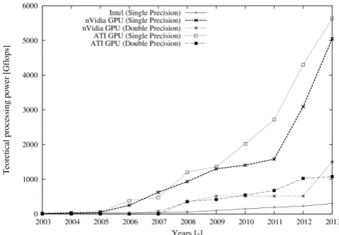
N recent years the dynamic development of multicore processors has had a direct impact on the availability of advanced high performance solutions for engineers. A few years ago, computers with a high-end graphics card were intended primarily for computer game players and computer graphics designers. Nowadays, the situation has dramatically changed. Graphic processors (GPUs – Graphics Processing Unit) are increasingly being used in high performance com-putations. A single GPU has a theoretical computational power several times higher than the fastest general purpose processors available today. Fig. 1 shows the increase in the theoretical computational power of graphic processors and general purpose processors in recent years. Computa-tions using a GPU working as a computing accelerator do not require any additional equipment, such as specialized workstations, and can be made on an ordinary personal computer equipped with a graphic card that supports CUDA or OpenCL. As graphic processors, in accordance with their original purpose, have been designed to efficiently perform mathematical operations on two-dimensional matrices, they should be capable of performing numerical simulations. The application of modern multi– and many–core architectures, such as graphic processors, for computational purposes al-lows huge systems of equations, which may consist of manyManuscript received December 20, 2013; revised January 08, 2014. Grzegorz Michalski is with the Czestochowa University of Technology, Dabrowskiego 69, PL-42201, Czestochowa, Poland. (corresponding author: Grzegorz Michalski; phone: (+48 34) 3250589; fax: (+48 34) 3250589; email:[email protected]).
[image:1.595.304.544.165.331.2]Norbert Sczygiol is with the Czestochowa University of Technology, Dabrowskiego 69, PL-42201, Czestochowa, Poland. (email:[email protected])
Fig. 1: An increase in theoretical computational power of the GPU and CPU in the recent years
millions of variables, to be solved very fast. The algorithms used for solving such systems of equations are based pri-marily on standard arithmetic operations on matrices and vectors. Such algorithms permit efficient parallelization and implementation for many–cores architecture like graphic processors. [1].
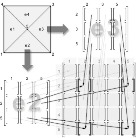
Fig. 2: Process of building the global coefficient matrix
II. BUILDING THE SYSTEM OF EQUATIONS ON GRAPHIC PROCESSORS
While performing simulations of unsteady processes the system of equations has to be built many times (for each time step). Owing to the specific nature of the graphic processors architecture, this can constitute a real problem and can significantly decrease the efficiency of computations. This relates to the slow data transfer from the global memory of the graphic devices (device memory) to the system mem-ory (host memmem-ory), synchronize mechanism and conditional instructions.
As the data transfer from the system memory to the global memory of the graphic devices should be reduced to a minimum, a good solution is to transfer the description of the finite element mesh to the graphic device global memory and build the system of equations using the graphic processor [4], [5], [6]. However, it should be remembered that the finite element meshes that are used nowadays often consist of a few million nodes. Transferring such a large amount of data is a very time–consuming process and, moreover this data can reduce the limited resources of the device.
The parallelization operation of the matrix building pro-cess on the basis of the finite element mesh is very compli-cated. This process requires a lot of conditional instructions and synchronize blocks, which causes a significant decrease in the performance of computations made on the graphic processor (nVidia GT200 in this case).
The values of elements in i–row of the coefficient matrix depend on the finite elements, which include the node connected with the node with index i. A single node in the finite element mesh can belong to several finite elements. No direct method exists to identify these finite elements solely on the basis of the node index. These indices can only be read from the finite element mesh. Fig. 2 shows the process of building the global coefficient matrix. Non–zero elements of the global coefficients matrix are determined as the sum of several values which depend on those finite elements
which include the pair of nodes with indexes corresponding to the indexes of the row and column of those elements. Constructing the global matrix of coefficient in this way definitely makes the parallelization process more difficult.
The approach presented in this paper uses a modified way of building the system of equations which divides this pro-cess into two separate phases. The first requires information from the finite element mesh. This phase is performed only once at the beginning of the computer simulation. An appro-priate transformation of the matrix obtained from the Finite Element Method makes this part of the matrix independent from the nodal temperatures and enthalpy values, determined in subsequent time steps. The second phase is performed in each time step and is dependent on the nodal temperature values and enthalpy from previous steps.
A. Two–step building of the system of linear equation
The system of equations resulting from the transformation of a differential equation, which describes the process of solidification, into the numerical model using the Finite Element Method can be finally written in matrix formulation (1) [7], [8], [9].
MHn+1+ ∆tKnTn+1=MHn+ ∆tbn+1 (1)
The elements of (1), which are built on the basis of the finite element mesh description are: matrix M (2) and conductivity matrixK(3) [10].
Me=
Z Ωe
NTNdΩ (2)
Ke(T) =
Z Ωe
λ(T)∇TN· ∇NdΩ (3)
MatrixMis independent from the nodal temperature and enthalpy values in subsequent time steps. This matrix may be determined at the beginning of the simulation, before the first time step is executed. This matrix can be used in the same form in the subsequent time steps. MatrixM is a diagonal matrix, and it is preferable to store it in the form of a simple vector, as this helps to save priceless graphic device memory. In contrast, conductivity matrixKis a temperature func-tion. The element which causes this dependency is thermal conductivity coefficientλ. The value of the thermal conduc-tivity coefficient is determined during the building of the matrix of coefficients for each finite element. If thermal conductivity coefficient λ is not dependent on the spatial coordinates, it can be taken out before the integral. After completing these steps, equation (3) assumes the form (4).
Ke=λ(T)
Z Ωe
∇TN· ∇NdΩ (4)
After integration, conductivity matrix K (for triangular elements) takes the form (5), whereKeis a local coefficient
matrix for the finite element,Athe surface area of the finite element, Cij are coefficients which depend on the spatial
Ke= λ(T) 4A
C2
21+C312 C21C22+C31C32 C21C23+C31C33
C21C22+C31C32 C222 +C322 C22C23+C32C33
C21C23+C31C33 C22C23+C32C33 C232 +C 2 33
(5)
Ke= 1 4A
λ1(C212 +C 2
31) λ1(C21C22+C31C32) λ1(C21C23+C31C33)
λ2(C21C22+C31C32) λ2(C222 +C 2
32) λ2(C22C23+C32C33)
λ3(C21C23+C31C33) λ3(C22C23+C32C33) λ3(C232 +C332 )
(6)
coefficient matrices, they are assembled into a global matrix of coefficientsK, which contains elements that are the sum of the products (their factors are different thermal conduc-tivity coefficientλ). These are average values calculated for each finite element that includes the corresponding nodes. Such a situation makes it impossible to separate this part of the matrix, which is temperature–dependent, from that part which is built on the basis of information contained in the finite element mesh.
In order to find a solution to this problem the authors have developed an alternative approach to the building of the system of linear equations. This approach allows the two parts of conductivity matrix K to be separated. It involves the introduction into the local matrices, values of the thermal conductivity coefficient λdetermined for the nodes and not for the finite elements as in the original approach. After this change is introduced into the equation (5) it takes the form (6).
This approach permits the removal of thermal conductivity coefficientλbefore the parenthesis in each element of global matrix K. After these steps the solidification equation in matrix formulation (1) takes the form described in equation (7).
MHn+1+ ∆tλnK∗Tn+1=MHn+ ∆tbn+1 (7)
where λ is the diagonal matrix of the thermal conductiv-ity coefficient for each node of the finite element mesh, determined on the basis of nodal temperatures from the appropriate time–step,K∗is a matrix of coefficients built on the basis of the finite element mesh description. MatrixK∗is
built only once at the beginning of the computer simulation. This approach allows the process of building the global coefficient matrix to be divided into two phases. The first phase is independent from the nodal temperatures values, and thus simultaneously independent from the time steps. Phase one is performed only once before the first time step of the simulation is performed. In this stage, matrix K∗ is built on the basis of information from the finite element mesh. Additionally, matrix B (calculated on the basis of the boundary conditions), diagonal matrixMand the vector (calculated on the basis of the boundary conditions) with values necessary to build the vector right sides in each time step are created in this stage.
After this step, the information stored in the mesh of finite elements (coordinates of the nodes, finite element descriptions, edges and areas) is no longer required for the process of computer simulation. The second phase of the matrix building process consists of determining conductivity coefficientλfor each node. As a result of this step diagonal matrix λ is created. This matrix is multiplied by matrix
K∗. As a result of the implementation of these operations
the non–zero elements of matrix K∗ are multiplied by λ values determined for the node whose index corresponds to the number of the row of the matrix. Since conductivity coefficient matrixλis temperature dependent, this operation must be performed in each subsequent time–step.
This approach simplifies the process of building the global matrix of coefficients on graphic processors by allowing matrixK∗ to be built on a general purpose processor.
B. Impact of the two–step building of the system of linear equation on the simulation results
The modifications to the numerical model produce slight differences in the temperatures in the nodes. However, these are just minor differences that do not affect the simulation of the casting solidification process. These differences result from the different way in which the value of the coefficient of thermal conductivity sensor is determined for the node, and not for the finite elements. This leads to a speed up in somputations performed in a sequential way (on the CPU ).
III. EXPERIMENTAL NUMERICAL VERIFICATION
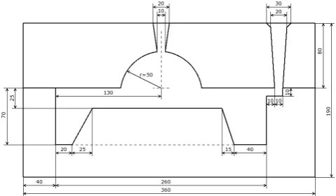
Simulations of the solidification process were carried out for the region shown in Fig. (3). Calculations were performed with the use of 6 finite element meshes, whose sizes ranged from several thousand to several hundred thousand nodes.
Times of simulations performed with the GPUs were compared to the results obtained with the authorial CPU– based sequential software. This software uses the approach to building the system of equations which was presented in previous section. The authors used a Boost Math library for matrix and vector calculations in the sequential implementa-tion. It should also be noted that all matrices are stored as sparse matrices using Compressed Sparse Row format.
[image:3.595.306.546.613.753.2]The computer simulation on the graphics processor was performed an nVidia GT200. The GPU–based casting solid-ification simulation software was run on the graphic devices:
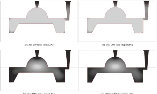
(a) after 200 time–steps(CPU) (b) after 200 time–steps(GPU)
[image:4.595.47.552.62.364.2](c) after 6000 time–steps(CPU) (d) after 6000 time–steps(GPU)
[image:4.595.52.286.409.578.2]Fig. 4: Distribution of the solid phase
Fig. 5: Speed up obtained with the use of GPU-based simulation software
1) nVidia TESLA C1060 (4 GiB GDDR), 2) GeForce GTX 260 (896 GiB GDDR).
Both the above are equipped with an nVidia GT 200 pro-cessor with 240 CUDA cores which has a peak performance of about 1 Tflops in single float operations. The authors used CUDA version 3.2 in the graphic processor implementations. The casting material is aluminum alloy with the addition of copper and the mold is assumed to be made from steel. The material properties are listed in Table I. The initial temperature of pouring was equal to 960 K and this value was the value of the initial condition temperature for the region of the cast in the performed calculations. The initial temperature
TABLE I: Physical properties of cast material (Al-2%Cu), and mold
Quantity Unit symbol Value Thermal Conductivity of solid phase mW·K 262 Thermal Conductivity of liquid phase mW·K 104
Density of solid phase kg
m3 2824
Density of liquid phase mkg3 2498
Specific heat of solid phase kgJ·K 1077
Specific heat of liquid phase kgJ·K 1275
Solidus temperature K 853
Liquidus temperature K 926
Melting temperature of pure metal K 933
Latent heat of solidification kgJ·K 390 000
Thermal conductivity of mold mW·K 40
Density of mold mkg3 7500
Specifiv heat of mold kgJ·K 620
of the mold was set at 560 K. Newton’s boundary condition is assumed on all the surfaces of the mold, assuming heat exchange with the environment with a coefficient equal to 100 mW2·K. The ambient temperature has a value of 300 K
in all boundary conditions. The heat exchange between the casting and the mold is obtained from a type IV boundary condition, which assumes the heat exchange through the in-sulation layer of the conductivity coefficient of the separating layer to be 800 mW2·K.
[image:4.595.309.542.436.611.2]taken to copy the data from the system memory to GPU memory and to copy the results into the system memory from the graphic device memory (first and last time–step). No differences were noted in the process of the computer simulation implemented on a general purpose processor and graphics processor. The simulation results (temperature and part of the solid phase) show that there is a slight difference between the results obtained with the GPU–based and CPU– based software. These differences are minor and do not exceed 0.1% and have no effect on the simulation process. This is illustrated in Fig. 4 which shows a part of the solid phase after 200 and 6 000 time–steps of computer simulation of the casting solidification process realized on CPU (Fig. (4a) and Fig. (4c)) and GPU (Fig. (4b) and Fig. (4d)). Comparing these figures it can be seen that the simulation process in both cases is the same.
IV. CONCLUSION
In this article, the authors present a new method of parallelization for the computer simulation of the casting solidification process and its implementation on graphics processors compatible with CUDA architecture. The pro-posed method divides the process of building the system of equations into the two phases. This solution improves the efficiency with which the available system resources are used. The great advantage of the developed solution is that it is easily adapted to the different architectures of multicore processors.
The speed up observed during the computer simulation of the casting solidification process confirms that the use of graphic processors in engineering simulations brings sig-nificant benefits. It was also noted that with an increase in the number of unknowns in the system of equations, the time needed to solve such a system increases linearly. At the same time, as the size of the task increases so does the speed up observed in the computations with the graphic processor.
Having regard to the the above results it can be stated that using graphic processors in engineering simulations seems to be a viable solutionas this approach can significantly reduce the time needed for research.
REFERENCES
[1] R. Strzodka, M. Dogger, and A. Kolb, “Scientific computation for simulations on programmable graphics hardware,”Simulation Model-ing Practice and Theory, vol. 13, pp. 667–680, 2005.
[2] S. Che, M. Boyer, J. Meng, D. Tarjan, J. W. Sheaffer, and K. Skadron, “A performance study of general-purpose applications on graphics pro-cessors using cuda,”Journal of Parallel and Distributed Computing, vol. 68, no. 10, pp. 1370–1380, 2008.
[3] nVidia,CUDA C Best Practices Guide v3.2, 20 August 2010. [4] P. Posp´ıchal, J. Schwarz, and J. Jaroˇs, “Parallel genetic algorithm
solv-ing 0/1 knapsack problem runnsolv-ing on the GPU,” in16th International Conference on Soft Computing MENDEL 2010. Brno University of Technology, 2010, pp. 64–70.
[5] C. Lee, X. Wei1, J. W. Kysar, and J. Hone, “Measurement of the Elastic Properties and Intrinsic Strength of Monolayer Graphene,”Science, vol. 321, pp. 385–388, 2008.
[6] nVidia,Optimization. OpenCL Best Practices Guide, 27 May 2010. [7] N. Sczygiol,Numerical modelling of thermo–mechanical phenomena
in a solidifying casting and mold. Wydawnictwo Politechniki Czestochowskiej, Czestochowa 2000. (in Polish).
[8] N. Sczygiol and G. Szwarc, “Application of enthalpy formulations for numerical simulation of castings solidification,”Computer Assisted Mechanics and Engineering Sciences, vol. 8, no. 1, pp. 99–120, 2001. [9] O. Zienkiewicz,The finite element method, Volume I, the Basis, 5th
ed. Oxford: Butterworth–Heinemann, 2003.