Cost-Efficiency Method for Production Scheduling

Cost-Efficiency Method for Production Scheduling

Y. Mauergauz

Abstract – This paper seeks to determine a dynamic Pareto-optimal method for various problems of production scheduling, based on simultaneousapplication of two criteria: relative manufacturing cost criterion and average orders utility criterion. In this method the concept of production intensity as a dynamic production process parameter is used. The method is applicable both for “make-to-order” and “make-to-stock” manufacturing strategies. The software used allows scheduling for middle quantity of jobs. The result of software application is the set of non-dominant versions proposed to a user for making a final choice.

Index Terms – Parallel machines, Pareto-optimality, production intensity, scheduling, single machine

.

I. INTRODUCTION

All possible quality criteria of the first SCOR model level relate to one of the four categories: customer service, economical indices, demand satisfaction flexibility, product development. The criteria of the last category are not usually considered in production planning, and demand satisfaction flexibility is ensured by strategy selection – “make-to-stock” or “make-to-order”. Therefore production planning quality mainly depends on the customer service level and production cost. The high customer service level (efficiency) may only be achieved through timely order completion. However, prompt order completion contradicts high level of utilization and increases expenses. This trend is known as ‘dilemma of operation planning’ [1].

In the last years some researches were have been conducted in order to solve the ‘dilemma of operation planning’, which studied multicriteria scheduling. Solution of this problem to a considerable extent depends on the chosen criteria of schedule quality. The main criteria used were overall production time or makespan

C

_max, the

highest tardiness

T

_max, average tardiness

T

, etc. A typical example of such method was demonstrated in the article by [2], where for a single machine three criteria were used: the criterion of “First In, First Out” or FIFO; the criterion of relative setup time SSU+ and the critical ratio criterion CR. The SSU+ criterion is the ratio between setup

time

s

_i and total job duration



p

_ifor a single job type.

Due to high complexity of this problem, appropriate researches mainly apply various heuristic methods. Some of these methods are aimed at finding Pareto optimal solutions for two selected criteria. In some instances a set of criteria was reduced to a single generalized criterion by means of their summation with a different weight for each criterion

Manuscript received February 04, 2013; revised April 03, 2013. Y. Mauergauz is with Infosoft Company, Moscow, Russia (e-mail: [email protected])

For instance, criteria of total tardiness



T

_i , total

cycle duration



F

_i and summary machine load

K

are

often used for a single machine.

For parallel machines this problem was considered as a problem with a single criterion created by linear

combination of initial criteria [3]. The ant colony system

algorithm was applied for a flow shop [4] with respect to both makespan and total flowtime as optimization criteria.

The above criteria are indirect criteria and do not reflect SCOR model requirements directly. Therefore some recent articles [5] were dedicated to scheduling by direct application of the cost criterion and the timely service criterion. For this purpose the mentioned paper describes a rather complicated system for sequential planning.

Reduction of costs in scheduling may be achieved through technological grouping of jobs, which provides for low setup time needed to shift from a job to a job within the group. As it was shown in the article by [6], the criterion of relative setup expenses

U

and the criterion of average

orders utility

V

may be considered for group scheduling. This paper demonstrates possibility to apply these criteria for certain scheduling problems.

The remainder of this paper is organized as follows. In Section 2 the problem is formulated, the function of direct expenses and the function of current orders utility are determined. Section 3 is dedicated to group scheduling for a single machine. In Section 4 group scheduling for parallel machine is considered. Section 5 is dedicated to jobshop production scheduling. Section 6 contains some concluding remarks.

II. UTILITY FUNCTIONS IN SCHEDULING

Assume we are drawing up a plan at

t

= 0, and certain job due dates have already expired, i.e. some d_i 0. Accordingly, it is necessary to use the dynamic customer service criterion, which is valid in the range of due dates

i

d    .

The customer service level may be assessed by the current order utility function V. From the manufacturer’s point of view, the order value increases proportionately to work amountpi, since staff engagement increases. Besides,

the more is the time reserve for completing an order, the more attractive is the order, since there is an opportunity to prepare for order execution. Eventually the order time reserve is decreasing, and the order value is diminishing. After all, if the due date has expired, the order value becomes negative.

1

( ) / 1

i i i

i w p H

G d t



G



 

at di  t 0

and

( 1)

i i i

i

w p t d

H

G



G



 

at

d_i t 0,

(1)

where p_i – processing time of job

i

, w_i– priority

weight coefficient of job

i

, G – plan bucket duration,



– “psychological coefficient”.

Fig. 1. Production intensity diagrams

Fig. 2. Current order utility function

The curves in Fig. 1 differ in the psychological coefficient value. The psychological coefficient determines the degree of placidity, when the time reserve is more than zero, and the degree of nervousness, when the time reserve is less than zero. The higher is the



coefficient, the more placid is the attitude to delays and the lower is the intensity.

Due to its additivity property, the production intensity may be used to describe status of planning objects and to assess various production environments: to compare intensity at various facilities (work centers, shops, departments). The production intensity concept may be used for determination of the current order utility function V (Fig. 2). Assume that the current utility for an order

i

is

i i

i i

w p

V H

G

 

.

(2)

The curve in Fig. 2 for the positive value d_i t 0 tends to the horizontal asymptote

/ i i i

V w p G

.

(3)

In the negative part d_i  t 0 the curve turns into the straight line with

i tg



 w pi ₂i

G



.

(4)

Now let us consider the nature of utility function change in the period from job execution start until its completion. Let the point A in the positive field correspond to the start of the job

i

with the processing timep_i. During job execution the remaining p_i decreases in a linear manner. However, since production intensity increases in time, the current order utility V_i would decrease in time ( d_it) during p_i in a non-linear mode as depicted by a dashed lineAB. Similarly, if job execution starts at the point C in the negative field in Fig.

2, the current order utility V_i would increase along a dashed line CD.

Assume that the order quantity on the planning horizon equalsN. Then their total utility V amounts to the sum of all order utilities, because orders, as a rule, are independent:

1 1 1

1

.

N N N

i i i i

i i i

V V w p H

G

  













(5)

The value of the function V changes in time since the time reserve until the moment of scheduled completion also changes. Besides, some orders are get completed, and new orders appear in time.

Let us assume that a certain job that corresponds to the node of the scheduling versions tree at the level l is completed at the moment of timeC_l. Let us also assume

that the job k starts at the moment t_k, which is more than

or equal toC_l. Then the average utility of the entire set of jobs J from starting until completion of the job k in the node at the level l1 equals

1,

0

1 1

( )

k k k k

l

t p t p

l k l l k

k k k k _C

V Vdt V C V dt

t p t p

 

    









.

(6)

In the formula (6) the value V_l equals to the average utility of the entire set of jobs on the planning horizon from the start moment t = 0 until completion C_l of the last scheduled job. For example, at the moment t = 0 the machine is available, the quantity of completed jobs is l = 0, and C₀= 0 accordingly. The value of t_k depends on the

1

k k k k k k

l l

l l l

t p t p t p

k i i i

i J I i J I

C C C

V dt w p dt H dt

G        













, (7)

where I_l – the set of jobs that would be completed in

accordance with scheduling before the moment t_k.

Possible versions of using the formula (7) for a single machine and rules to compute integrals it contains are described in [8].

The function of negative expenses utility (loss function) for a single machine may be used as the first criterion in the dilemma “cost / efficiency”. If the sequence number of planning job is n

0 0

1

[ ( )]

n n

s l r kl l

l l

U c s c t C

c _{ }









 , (8)

where c_s– cost of setup time unit, c_r– cost of idle time

unit, s_l– setup time on level l.

Therefore, the scheduling optimization for a single machine may be achieved with the highest possible value of average orders utility V and the least possible value of expenses U on the planning horizon h. In this process, V has to be computed according to the formula (6), U- according to the formula (8) at every level of the possible solution tree.

III. GROUP SCHEDULING FOR SINGLE MACHINE

Assume there is a set of jobs that arrive to a machine for processing in any sequence. These jobs refer to any of S

various types. The setup time s_fq depends on sequence of

transition from a type f to a type q; when a job is available, the machine may also be idle, this results in additional costs. In accordance with the well-known three-part scheduling classification, the considered problem is: 1| ,r d si i, fq|U V, . (9)

There are two target functions in the formula (9), and they may both be improved only within certain limits. The Pareto compromise curve serves as such limit, because in its points the criterion Uimprovement (diminution) means the criterion V deterioration (diminution). For solving the problem (9) it makes sense to apply the method, based on the MO-Greedy approach [9], which requires building a tree to search for non-dominated solutions. Using the expressions (1, 2), (6, 7) and formulas in [8], we can calculate the criterion V value in every tree node. The criterion U value may be computed by the formula (8) in every node as well.

Now it is possible to formulate the MO-Greedy algorithm for solving the problem.

Step 1. (Initial computation of utility functions)

Let us suppose that the level number is l=0; the machine is available, so C_l=0; the initial expense function value is U₀=0; the initial orders utility function V₀ may be computed by the formula (5). Step 2. (Utility function computation at next levels)

For each job k that arrived before the moment C_l and

has not yet been completed, values U_l1,k and V_l1,k

are computed using the formulas (8) and (6). Step 3. (Determination of dominated tree nodes)

If the level l 1 N, then for domination on the level 1

l of the tree node j with a job i over the tree node r with a job k it is sufficient to comply with the following inequations

1, 1,

l j l r

U_ U_ ,Vl1,j Vl1,randg_ig_k, (10)

besides, the first or the second inequation is strong. Otherwise: on the last level l 1 N domination is possible, if

1, 1,

l j l r

U_ U _ , Vl1,j Vl1,r. (11)

Step 4. (Transition to the next level or stopping) Level number increment l l 1.

If the level is lN, then STOP. Otherwise, go to Step 2.

The inequation (10) applies the necessary start moment

i

g , which is determined as

gi = di – pi. (12)

Let us consider the following example assuming it is possible to perform three types of jobs on a single machine, where the setup time is sequence-depending. In Table I there is a list of five jobs to be scheduled within the 7-hours horizon. The norms of setup time

s

_fqchange from 0.1 to

0.3.

Table I Job characteristics

Job 1 2 3 4 5

Product type 1 2 1 3 1

Processing time

pi, hours 1 2 1 2 1

Due date di -1 2 3 3 6

Time of job

arrival ri -4 0 1 1 2

Necessary start

time gi -1 1 3 2 6

Fig. 3. Computation results for data in Table I

Fig. 4. Diagrams of scheduling versions 1



4 utility; a - horizon 6; b– horizon 7; c– horizon 8.

Every sequence version 1



4 corresponds to a trajectory on the plane of the average order utility criterion

V and the relative cost criterion U, as shown in Fig. 4. By joining the points for different versions that correspond to the same horizon, it is possible to depict the set of Pareto-optimal solutions. In Fig. 4 such compromise curves а, b, c for horizons 6, 7, 8 are drawn accordingly.

Analysis of the diagrams in Fig. 4 makes it possible to make some conclusions about properties of solutions on the

U Vplane. The average orders utility of V decreases at every subsequent horizon. This is quite natural, since the time reserve for order completion decreases. At the same time the relative cost U increases. Sparseness of version points in the plane increases together with the horizon.

IV. GROUP SCHEDULING FOR PARALLEL MACHINES AND “MAKE-TO-STOCK” MANUFACTURING STRATEGY

The average job i processing time for parallel unrelated machines equals to

1 1 m

i ij

j

p p

m _





, (13)

where p_ij – processing time of a job i on a machine j. When scheduling for the “make-to-stock” strategy

orders of customers are not considered. At the same time it does not mean that a planner may neglect them. When the “make-to-stock” strategy is used, it is necessary to provide (if applicable) the sufficient stock of every manufacturing product during the whole manufacturing time. Such stock has to provide for both satisfaction of expected average demand and minor demand deviations of average values. For the last purpose it is necessary to provide a certain safety stock.

For parallel machines the recurrent formula (6) may be used without changes, if completion of a job on the previous level l happens before job completion on the

subsequent l1 level. Otherwise, instead of the formula (6) the following formula is used

1, 1

k k

jq t p

l k l _k

il _C

V V V dt

C



  



, (14)

wherei – the machine number in the tree node, from which a new branch grows; j– the machine number, for

which a new job Jk in a new branch is meant; Cil - the

end of machine i operation on the levell; C_jq- the

completion time of the last job, which was planned on the level qon the machine j.

The algorithm for this problem is similar to the algorithm for the single machine problem. The difference consists in the necessity for node branching for every parallel machine.

Let us consider the task of scheduling for six parallel unrelated machines and products of six various types. Assume that manufacturing of any product on every machine is only possible in a volume larger than a so called “technical lot”. This lot may equal to the machine volume (for process manufacturing), the package quantity for discrete manufacturing, the transit norm (for instance, by weight), etc. Duration of technical lot manufacturing correlates with technical parameters of the machine and depends on the product type.

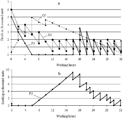
During task execution the stocks and backlogs of every product are changing. Apparently, the schedule is good, when average stocks are not high and there is no backlog. Fig. 5a presents three stock dynamics processes most typical for scheduling that describe processes for products P2, Q1 and R1. Process dynamic of products P1 and P3 to a considerable extent is similar to the process of the product Q1, the process of the product Q2 is similar to process of the product P2.

Fig. 5. Dynamics of stocks and backlog during the task execution

It follows from the diagrams in Fig. 5a that the most even is the process of manufacturing of the product R1, and there was no backlog of this product. Note that for the product R1 the highest safety stock is provided, which substantially caused such scheduling result. For the product Q1 the plan provides for manufacturing of high stock in the initial stage of the scheduling interval and then gradual consumption from this stock to the safety stock level. In this case there is no backlog as well.

[image:5.595.45.446.66.450.2]

The situation with the product P2 is much more complicated. According to the schedule, the initial considerable stock should be spent in six hours; then the backlog of this product arises and grows as shown in Fig. 5b. It is only possible to reduce the backlog of this product to zero at the end of the planning interval.

V. GROUP SCHEDULING FOR JOBSHOP MANUFACTURING

This problem may be considered as scheduling for several groups of parallel machines of various purposes. In this case every job consists of a set of operations, and every operation has to be executed on a machine with a corresponding purpose. Let us assume that a set of jobs for manufacturing may be divided into groups of several types,

and operation setup norms s_ij depend on the

corresponding machine group j and job kindi .

For example, let us consider scheduling for 20 jobs, each job contains from 3 to 5 operations to be executed in any given sequence. Assume there are 6 types of the job and the quantity of the machine group is 5. Table II specifies machine properties at the start of scheduling.

As it follows from Table II, there are 2 machines in the group 1, the group 2 includes 3 machines, there are 2 machines in the group 4 and each other group includes one machine. Besides, the machine 2 in the group 1 and

the

machine 4 in the group 2 are excluded from planning.

Table II Machine properties at scheduling start

Machine number

Number of machine

group

Start point

Settings at start

Release moment

Fig. 6. Scheduling results for one of non-dominated versions

Fig. 7. Gantt diagrams for two machines

Applying of the scheduling method described above produces two non-dominated versions of a schedule and one of them is given in Fig. 6 as a record in the MS Excel sheet. Numbers in the sequence for every machine correspond to the number of a job and (in a fraction) the operation number of this job to be completed on this machine. Numbers in brackets form a group of jobs of identical type that do not require setup.

In Fig. 7 the Gantt diagrams for the machines 1 and 3 are depicted. Rectangles in the diagrams correspond to working operations, gaps stand for idle time. Thick lines correspond to operations without setups as their job type is the same as the previous one.

VI. SUMMARY AND CONCLUSION

We have studied the dynamic method to solve the “operation planning dilemma” for a single machine, parallel machines and jobshop manufacturing. The relative expenses

U criterion and the average orders utility V criterion are used to define the correlation “cost/efficiency” on the planning horizon. The average orders utility value is determined, depending on the production intensity H_i of every order, which changes in time. To design a schedule, a set of Pareto-optimal solutions shall be calculated on the planning horizon, and the final decision shall be made by the user.

The described method has considerable advantages compared to others due to an option of scheduling jobs with negative due dates. Besides, the method allows analyzing

values of relative setup cost and the average orders utility in order to choose the most acceptable schedule version.

For a single machine this method may by applied both for series-batch and parallel-batch fulfillment of various jobs. Quantity of possible jobs in the last case is determined by the machine work size and size of batches to be processed. Computations show that the suggested method of scheduling for a single machine is suitable in the large parameter interval.

If a flowshop manufacturing is the case, it may be considered as a particular case of jobshop manufacturing with uniform operation sequence for corresponding machine groups. Therefore the suggested method may be applied for flowshop manufacturing both for “make-to-order” and “make-to-stock” manufacturing strategies. In real practice various additional constraints may be necessary for scheduling. For example, often it is needed to take into account the current device wear and tear, limited storage possibilities, general shipping terms, etc. In our opinion, it is reasonable that a user and the primary developer work out a customized program for every particular case.

REFERENCES

[1] Nyhuis, P. and Wiendal, H.P. (2009) Fundamentals of Production Logistics, Berlin: Springer.

[2] Ang, A.T.H., Sivakumar, A.I. and Qi, C. (2009) ‘Criteria selection and analysis for single machine dynamic on-line scheduling with multiple objectives and sequence-dependent setups’, Computers & Industrial Engineering, Vol. 56, No. 4, pp.1223–1231.

[3] Bozorgirad, M. A. and Logendran, R. (2012) ‘Sequence-dependent

group scheduling problem on unrelated-parallel machines’, Expert

Systems with Applications, Vol. 39, No. 10, pp. 9021-9030.

[4] Yagmahan, B. and Yenisey, M. (2010) ‘A multi-objective ant colony system algorithm for flow shop scheduling problem’, Expert Systems with Applications, Vol. 37, No.2, pp. 1361-1368.

Manufacturing Industry Test Operation’, Applied Mechanics and Materials,Vols. 110-116, pp. 3922-3929.

[6] Mauergauz, Y. (2012) ‘Objectives and constraints in advanced planning problems with regard to scale of production output and plan hierarchical level’ Int. J. Industrial and Systems Engineering, Vol. 12, No. 4, pp.369-393.

[7] Mauergauz, Y. (1999) Information Systems of Industrial Management, Moscow: Filin. (in Russian).

[8] Mauergauz, Y. (2012) Advanced planning and scheduling in manufacturing and supply chains, Moscow: Economica. (in Russian). [9] Canon, L.-C. and Jeannot, E. (2011) ‘ MO-Greedy: an extended

beam-search approach for solving a multi-criteria scheduling problem on heterogeneous machines’, In the IEEE International Symposium on Parallel and Distributed Processing Workshops and PhD Forum,