Changes in a river’s regime of a watercourse after a small water reservoir construction

(1)

Changes in a river’s regime of a watercourse

after a small water reservoir construction

Rostislav Fiala

1

_{, Jana Podhrázská}*

2

_{, Jana Konečná}

2

_{, Josef Kučera}

2

_,

Petr Karásek

2

,

Pavel Zahradníček

1

, Petr Štěpánek

1

1_{Czech Hydrometeorological Institute, Brno, Czech Republic}

2_{Research Institute for Soil and Water Conservation, Brno, Czech Republic} *Corresponding author: rostislav.fiala@chmi.cz

Citation: Fiala R., Podhrázská J., Konečná J., Kučera J., Karásek P., Zahradníček P., Štěpánek P. (2020): Changes in a river’s regime of a watercourse after a small water reservoir construction. Soil & Water Res., 15: 55−65.

Abstract: The paper deals with the analysis of a river’s regime of a small watercourse and the evaluation of its changes after the construction of a small water reservoir. The aim of the work was to analyse 12 years of flow rate measure-ments at two profiles of a small watercourse, between which a small water reservoir was built, in the middle of the period of the measurements. The analysis uses traditional characteristics (average flow rate, discharge volume), as well as modern indices from applied hydrology (Richards-Baker flashiness index, hydrogram pulse analysis), which study the variability of the flow rate in hourly and daily intervals. The evaluation showed that at the average flow rate, the effect of the water reservoir was the smoothening of the peak flow rates and prolonging the duration of the discharge waves. At higher flow rates, the water reservoir causes a delay in the culmination and in terms of discharge balance causes a decreased discharge volume, in particular during the vegetation period.

Keywords: hydrological characteristics change; flashiness index; hydrogram pulse; vegetation period

Supported by the Ministry of Agriculture of the Czech Republic, Project No. MZE-RO2018, and by the Technology Agency of the Czech Republic, Project No. TACR TH 04030363.

The precipitation-runoff processes in small agri-cultural catchments have been a long-term studied question, especially in connection with the water basin siltation, water pollution and the degradation of the soil by erosion. At present, the agricultural practice in the Czech Republic especially empha-sises agrotechnical and organisational measures to prevent harmful surface runoff, to reduce the flow of pollutants and the removal of the most valuable soil components (Podhrázská et al. 2018).

However, in small agricultural catchments, espe-cially in areas with sloping plots, the response to precipitation episodes is relatively rapid and often results in floods (Kovář et al. 2015). These events result in environmental, social and economic dam-age to the affected area. The agricultural landscape

(2)

et al. 2015). Land consolidation measures not only aim at enabling the rational management of the land users, but also in increasing the ecological stability of the landscape, thus better resisting the extremes in a climate’s development (Chahine 1992). Janků

et al. (2014) also pointed out that land and

environ-ment protection is important for the public and for further sustainable development.

The function of a water reservoir, aimed as a flood control, should especially be to transform the flood wave so that it safely flows through the area below the reservoir, with which other authors agree, for example Jaroš et al. (2016). Flooding only occurs more than once a year at the same location very rarely and there are locations where floods have not occurred for many years again. This means that for most of the time, such a water reservoir serves differ-ent functions, for example, it is a landscape feature and it balances out the fluctuating flow rates. The ongoing evaporation from the free water surface and the surrounding vegetation also significantly affects the discharge balance of the surface water from the basin. Kovář and Bačinová (2015) found the same fact, with a large influence, especially in dry periods. An increase in the drought frequency, its duration and severity is expected for the Central European region as a direct consequence of climate change (Trnka et al. 2016)

MATERIAL AND METHODS

In response to the extreme rainfall and subsequent floods in the village of Sloup (Blansko district) and the surrounding area on May 13 and May 26, 2003, a study aimed at the flood control including a water reservoir construction close to the village of Němčice was devised. In 2005, experimental profiles were placed at a small watercourse in the location of the planned water reservoir, where the flow rate, precipi-tation, air temperature and suspended sediments were measured. The proposed water reservoir was built in 2011, located between these profiles (Figure 1)and the data is, therefore, available both before and after the existence of this new landscape feature (Table 1). There are many indicators and indices for calculating the nature of water flow patterns. However, some of them are not suitable for small river basins and some provide similar information. This may cause some subsequent analyses to be affected by the col-linearity and are, therefore, nearly unnecessary. The use of the indices should be chosen according to the purpose of the processing. (Olden & Poff 2003).

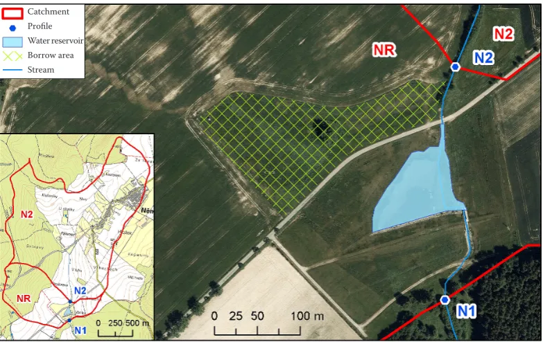
[image:2.595.106.498.478.725.2]

The watercourse of interest is a dynamic one, with a quick response to precipitation, in particular to tor-rential rains, however during the vegetation period, significant evaporation causes droughts during the summer time. The sewage system (including rainfall)

Figure 1. The experimental catchment and the water reservoir with grassed borrow area (source: Czech Office for Sur-veying Mapping and Cadastre, author)

(3)

from a small village and the ditches near the roads flow into the watercourse which causes a quick re-sponse to torrential rains. The overall surface area that was affected by the water reservoir construction (WRC) is approximately 6 ha (a small water reservoir and a littoral region of about 0.6 ha, a borrow area of about 2.1 ha and grassy vegetation near the water reservoir of about 3.3 ha).

The fundamentals for this analysis are a database of the daily rainfall and hourly and daily flow rates and discharge volumes from the two profiles lying 250 m apart at a small watercourse with a basin area of 350 ha (lower N1 profile) and 282 ha (upper N2 profile).

The continual flow rate and air temperature mea-surements have been recorded since April 2005. Gaps in the data are caused by instrumentation malfunctions (almost always in winter), theft of the measuring equipment and due to the construction of the water reservoir. The entire analysis only uses complete and suitable data. The database of precipi-tation has been reviewed and supplemented with a complete set of homogenised data from the Czech Hydrometeorological Institute (Štěpánek 2008; Štěpánek et al. 2009).

The initial data comparison was made using a com-parison of the basic dataset characteristics from both profiles – the average flow rate and the discharge volume. Then, the sums of the precipitation and the effective temperatures were calculated. The character-istics and indices were calculated for the hydrological years (r) and the seasons – the vegetation period (v), spring (MAM), summer (JJA), autumn (SON) and winter (DJF). The hydrological year begins on Nov 1 and ends on Oct 31 of the following year, the vegeta-tion period lasts from Apr 1 to Sep 30.

The short-term flashiness is well expressed by the Richards-Baker flashiness index (RB FI) (Baker et al. 2004), which is dimensionless. Its values range from 0 to 2, where 0 means a constant flow rate. For the calculation, one can use the average daily flow rate (Q_d) or the daily discharge volume (W_d) (marked as q in the original equation below). The

index can be calculated for seasonal as well as an-nual time periods.

(1)

The hydrogram pulse analysis (Archer & New-son 2002) can be used for the compariNew-son of several basins or several profiles on one river. This method is based on the frequency and duration of the pulses above selected threshold flows. A pulse is defined as an occurrence of a rise above a selected flow and the pulse duration is the time from when it rises above the threshold to the time it falls below the same threshold (Figure 2).

The thresholds are set as multiples of the median flow (M) as 0.5M, M, 2M, 3M, 4M, 5M, 6M, 7M, 8M, 10M, 15M, 20M, 30M, 40M, 50M, 60M, 80M and 100M. The median flow has been taken over the whole period. The data (flow in hourly steps) were analysed as a subset of all the data, separately for each hydrological year and vegetation period. For each period, the total number of pulses and the total duration above the threshold was counted and the average duration per pulse was computed. In order to perform the hydrogram pulse analysis, the periods of the same length has to be selected before and after the reservoir construction with the complete hourly flow data, which, moreover, is not burdened by the occurrence of extreme runoff situ-ations. The reason for this is for the comparability of the result for both profiles and the whole period RB FI = ∑

n

n=1|qi–qi−1|

[image:3.595.62.534.114.179.2]

∑nn=1qi

[image:3.595.304.530.633.721.2]

Figure 2. The definition diagram for the pulse numbers and the pulse duration (Archer & Newson 2002)

Table 1. Summary of complete the data

Hydrological years Vegetation period (IV–IX)

N1 Profile 2006, 2007, 2008, 2010, 2014, 2017 2005, 2006, 2007, 2008, 2009, 2010, _{2013, 2014, 2016, 2017}

N2 Profile 2006, 2007, 2008, 2010, 2011, 2012, _{2013, 2014, 2016, 2017} 2005, 2006, 2007, 2008, 2009, 2010, 2011, _{2012, 2013, 2014, 2016, 2017}

Time

Di

sc

har

ge 3 × Median

2 × Median

(4)

before and after the reservoir construction. From the entire dataset, only 2007, 2008, 2014 and 2017 were used for the hydrological year, and 2005, 2007, 2008, 2009, 2013, 2014, 2016 and 2017 were used for the vegetation period. At the end of the analysis, there is an overview of the relative changes in the N1 profile after the water reservoir construction.

All computations were performed in the software R (R Core Team 2018), for the homogenisation of the precipitation, the software ProclimDB (Štěpánek 2008) was used.

RESULTS

The following hydrometeorological characteristics were calculated from the complete measurement database in the vegetation period (Table 2).

[image:4.595.65.532.110.334.2]

In the summarised characteristics (Figure 3), the course of the average flow rate at the N2 profile more or less correlates with the rainfall (R = 0.756 for the hydrological year and R = 0.651 for the veg-etation period). The last dry years are characterised by high temperatures and low precipitation, which Table 2. The basic meteorological and hydrological characteristics for the vegetation period

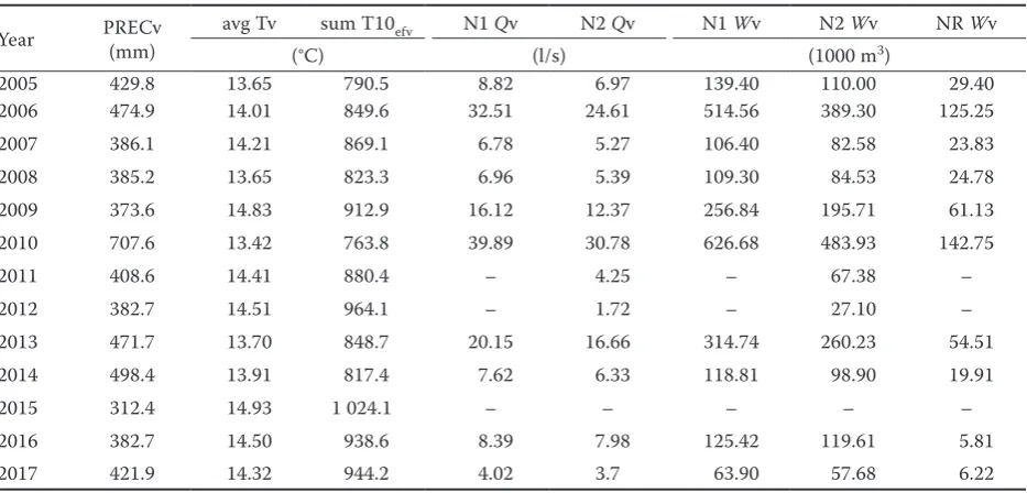
Year PRECv_(mm) avg Tv sum T10efv N1 Qv N2 Qv N1 Wv N2 Wv NR Wv

(°C) (l/s) (1000 m3₎

2005 429.8 13.65 790.5 8.82 6.97 139.40 110.00 29.40

2006 474.9 14.01 849.6 32.51 24.61 514.56 389.30 125.25

2007 386.1 14.21 869.1 6.78 5.27 106.40 82.58 23.83

2008 385.2 13.65 823.3 6.96 5.39 109.30 84.53 24.78

2009 373.6 14.83 912.9 16.12 12.37 256.84 195.71 61.13

2010 707.6 13.42 763.8 39.89 30.78 626.68 483.93 142.75

2011 408.6 14.41 880.4 – 4.25 – 67.38 –

2012 382.7 14.51 964.1 – 1.72 – 27.10 –

2013 471.7 13.70 848.7 20.15 16.66 314.74 260.23 54.51

2014 498.4 13.91 817.4 7.62 6.33 118.81 98.90 19.91

2015 312.4 14.93 1 024.1 – – – – –

2016 382.7 14.50 938.6 8.39 7.98 125.42 119.61 5.81

2017 421.9 14.32 944.2 4.02 3.7 63.90 57.68 6.22

PREC – the precipitation total; avg T – the average temperature; sum T10ef – the sum of the effectivetemperatures above 10°C; N1 – the lower profile; N2 – the upper profile; NR – the subcatchment between the profiles; Q – the average flow rate;

W – the discharge volume; the suffix “v” means the vegetation period

Figure 3. The overview of the selected hydrometeorological characteristics for the vegetation period

PREC – the precipitation total; sum T10ef – the sum of the effectivetemperatures above 10°C; N2 – the upper profile; NR – the subcatchment between the profiles; W – the discharge volume; the suffix “v” means the vegetation period

N

R

W

v (× 1000 m

3)

N2

W

v (× 1000 m

3)

PR

EC

v (mm)

sum T10ef

v (°C

[image:4.595.78.520.563.708.2]

(5)

is subsequently reflected in the decreased outflow from the basin to the water reservoir and also in the higher losses via evaporation from the water surface of the water reservoir. The most significant aspect is the decrease in the discharge volume from the basin between the profiles (NR Wv) in comparison with the discharge on the N2 profile (N2 Wv). Before the water reservoir, the discharge volume of the NR was about 30% of the N2 discharge volume. In 2013 and 2014, it was about 20% and, in 2016 and 2017, it was only 5 and 10%, respectively. The difference in 2016 and 2017 compared to 2013 and 2014 could be due to higher temperatures and evapotranspiration and lower precipitation.

[image:5.595.85.518.95.290.2]

The effect of the water reservoir construction can be seen in the actual hydrograms of hourly flow rate also (Q_h) (Figures 4 and 5), however, it is not so ap-parent in the case of the daily averages. During the periods of low flow rates (approximately up to 100 l/s at the upper N2 profile), the water reservoir’s effect is the lower culmination and smoothening of the flow wave. Similar results were published by Zhang et al. (2016). The wave smoothening was not observed at higher flow rates above 100 l/s (Figure 5), yet one could still see a decrease and a slight delay in the culmination. After the water reservoir construction, a flow rate of more than 1500 l/s was not observed, so the functionality of the water reservoir during Figure 4. The example of the hydrogram before (a) and after (b) the water reservoir construction

Q_h – the hourly flow rate; N1 – the lower profile; N2 – the upper profile

Figure 5. The example of the higher flow rate hydrogram

[image:5.595.76.526.541.720.2]

(6)

the flood period (flow rates in the range of a few to several tens of m3_{/s) could not be tested.}

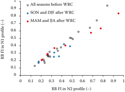
The Richards-Baker flashiness index (RB FI) char-acterises the commonly low flashiness of flow rate during winter and spring time (< 0.5), and the high flashiness during the summer (> 0.5) (Figure 6).

The flashiness during the summer and autumn most likely stems from frequent rains of various intensities and durations, which affect the flashi-ness of the flow rate on both profiles. In contrast, during the winter and spring months, the flow rate variability is decreased by the lower temperatures (frost, snow) and the gradual melting of the snow cover, which causes high flow rates in spring, how-ever, relatively constant.

The last few years show a big difference between the profiles in the summer, autumn and winter (Figure 7). In order to perform the hydrogram pulse analysis, the value of the median for the entire period of meas-urement has to be computed. The N1 and N2 values were computed for the hydrological year (4 years),

N1 Q_MEDr= 4.3 l/s, N2 Q_MEDr= 3.5 l/s, and for the

vegetation period (8 years), N1 Q_MEDv= 2.0 l/s, N2

Q_MEDv= 1.9 l/s.

The effect of the water reservoir construction (WRC) is the flow rate stabilisation below the reser-voir due to the balancing out of the flow rate flashiness above the reservoir. This can be seen in the results of the hydrogram pulse analysis also for hydrologi-cal years as well as for the vegetation periods, where one can see the changes in the position of the red solid line (the N1 profile after the water reservoir construction) in comparison with the other three lines on Figures 8–13. The M40 threshold was only exceeded 9 times in the selected hydrological years

and 34 times in the selected vegetation periods (ap-proximately about 2 and 4 occurrences per year, respectively) so the comments will be focused mostly on lower categories.

[image:6.595.65.527.96.243.2]

From the point of view of the number of pulses above the thresholds, in the hydrological years, a number of pulses on the N1 profile in the low flows is reduced by 37 to 48% in the categories up to 4M and by about 27.5% in the categories up to 10M. In the categories above 15M, the pulse counts have not changed, more or less. In the vegetation period, the 0.5M and 50M categories have shown a small decrease in the number of pulses only, in other cat-egories from 2M to 40M, a decrease of 35 to 56% Figure 6. Comparison of the Richards-Baker flashiness index (RB FI) for the seasons throughout all the years

[image:6.595.307.524.509.669.2]

DJF – the winter season; MAM – the spring season; JJA – the summer season; SON – the autumn season

Figure 7. Comparison of the Richards-Baker flashiness index (RB FI) for the seasons before and after the water reservoir construction (WRC)

DJF – the winter season; MAM – the spring season; JJA – the summer season; SON – the autumn season; N1 – the lower profile; N2 – the upper profile

0 0.1 0.2 0.3 0.4 0.5 0.6 0.7 0.8 0.9 1

RB FI

in

N

1

profil

e

(–)

RB FI in N2 profile (–) All seasons before WRC SON and DJF after WRC MAM and JJA after WRC

0 0.2 0.4 0.6

2005 2007 2009 2011 2013 2015 2017

RB

FI

(-)

Year DJF N1

N2

0 0.2 0.4

2005 2007 2009 2011 2013 2015 2017

RB FI

(-)

Year MAM

N1 N2

0 0.5 1

2005 2007 2009 2011 2013 2015 2017

RB F

I (

-)

Year JJA

N1

N2 ₀

0.5 1

2005 2007 2009 2011 2013 2015 2017

RB

FI

(-)

Year SON N1

N2

Year Year

(7)

[image:7.595.91.503.97.258.2]

Figure 8. The number of pulses above the threshold for the hydrological years

N1 – the lower profile; N2 – the upper profile; WRC – the water reservoir construction

Figure 10. The total pulse duration above the threshold for the hydrological year N1 – the lower profile; N2 – the upper profile; WRC – the water reservoir construction

0 20 40 60 80 100 120 140 160 180 200

>0.5M >1M >2M >3M >4M >5M >6M >7M >8M >10M >15M >20M >30M >40M >50M >60M >80M >100M

Nu

m

ber

o

f p

ulses

Multiplies of median flow

N1 before WRC N1 after WRC N2 before WRC N2 after WRC

N

umb

er of pul

se

[image:7.595.92.516.318.490.2]

s

Figure 9. The number of pulses above the threshold for the vegetation periods

N1 – the lower profile; N2 – the upper profile; WRC – the water reservoir construction

0 20 40 60 80 100 120 140 160 180 200 220 240 260 280

N

um

ber

o

f p

ulses

Multiplies of median flow N1 before WRC N1 after WRC N2 before WRC N2 after WRC

N

umb

er of pul

se

s

0 2000 4000 6000 8000 10000 12000 14000

To

ta

l p

uls

e d

ur

at

io

n (h

)

Tot

al pul

se dura

[image:7.595.87.501.547.721.2]

(8)

has been observed. The small flat part of the solid red line between 4M and 10M (Figure 8) may mean a common overrun of both thresholds.

In the hydrological years and the vegetation peri-ods, there is a little decrease in the total time of the duration of the pulses above the thresholds in almost all of the categories. But this fact is only relative because there is a large decrease in the number of pulses (Figures 10 and 11), so, the average duration of the pulses mostly increases (Figures 12 and 13).

In the hydrological years, the average duration of one pulse in the categories 0.5M to 10M is higher by an average of about 27% (+15 to +45%). In the 15M

category, it is virtually indistinguishable (+2%) and in the categories from 20M to 40M, it is lower by an average of about 79% (–33 to –70%). In the vegetation period, the average duration of one pulse is higher by 50 to 348%, except for the 30M and 50M categories where the increase is only 4 and 23%, respectively. The highest increase in the average duration is in the categories M2 and from M4 to M20 by an average of about 180% and the lowest increase is in categories 0.5M, 1M, 3M and from M30 to M60 by an average of about 49%.

After the water reservoir construction, the change in the N1 profile is seen more or less in all the

[image:8.595.73.519.285.469.2]

character-Figure 12. The average pulse duration above the threshold for the hydrological years N1 – the lower profile; N2 – the upper profile; WRC – the water reservoir construction Figure 11. The total pulse duration above the threshold for the vegetation periods N1 – the lower profile; N2 – the upper profile; WRC – the water reservoir construction

0 2000 4000 6000 8000 10000 12000 14000

To

ta

l p

ulse d

ur

at

io

n

(h

)

Tot

al pul

se dura

tion (h)

0 20 40 60 80 100 120 140

Av

er

ag

e

pu

lse d

ur

atio

n

ab

ov

e

thr

esho

ld

(h

)

Average pul

se dura

tion a

bove tr

es

[image:8.595.77.521.535.722.2]

(9)

istics of the hydrogram pulse analysis (Figure 14). The largest decrease in the number of pulses is up to 4M (17 l/s) in the hydrological years (about 47% on aver-age) and in the range from 2M to 20M (4 to 40 l/s) in the vegetation periods (about 50% on average). There is a large extension of the average pulse duration in the range up to 10M (43 l/s) in the hydrological years (about 27% on average) and up to 20M (40 l/s) in vegetation periods (about 160% on average).

DISCUSSION

Construction of the water reservoir also included construction of a borrow area (2.1 ha) between the

two profiles and creating a relatively large grassy area (approximately 3.3 ha). The borrow area has a flat bottom and is covered with a hygrophilous vegetation. Given its location in a thalweg between the two basins and given its nature it could affect the water regime and overall balance to a similar extent or even more than the actual water reser-voir. Bullock and Acreman (2003) and van der

Ent et al. (2014) have similar experiences. Its main

[image:9.595.80.514.100.280.2]

effect could be the capture of the water from the melting snow between the basins, the retardation of the discharge from the precipitation including torrential rains (the gradual release into the stream) and the support of the evaporation and infiltration Figure 14. The change in the N1 profile after the water reservoir construction

[image:9.595.76.519.341.518.2]

N1 – the lower profile

Figure 13. The average pulse duration above the threshold for the vegetation periods N1 – the lower profile; N2 – the upper profile; WRC – the water reservoir construction

0 10 20 30 40 50 60 70 80 90 100

Aver

ag

e p

ulse

du

ra

tio

n

ab

ov

e thr

esho

ld

(h)

N1 before WRC N1 after WRC N2 before WRC N2 after WRC

Average pul

se dura

tion a

bove tr

es

hold (h)

-100 -50 0 50 100 150 200 250 300 350 400

Chang

e

in

N1 af

te

r WRC (

%

)

Veg. period: number Veg. period: duration Veg. period: avg. duration Hydr. year: number Hydr. year: duration Hydr. year: avg. duration

C

hange in N1 af

ter W

(10)

of the water created in the basin between the two profiles. Kovář and Bačinová (2015) have similar experiences with evapotranspiration.

The Richards-Baker flashiness index is a relatively new characteristic, which shows the differences in the short-term watercourse flashiness, regardless of the overall size of the flow rate. It is, therefore, quite useful when comparing watercourses of differ-ent sizes. This was shown by Baker et al. (2004) in a study of watercourses in the Midwest U.S., where they compared 515 profiles at watercourses with a basin size ranging from 8.5 to 29 000 km2_{. Another}

advantage is that it is applicable for different time periods, not just the hydrological years, but shorter intervals also. A possible disadvantage is that the result of the analysis is a number with a relatively small variance (0.1 to 0.9, in the case of this paper), which may negatively affect its usability in regres-sion models. In this case, it could be better to use the hydrogram pulse analysis, which provides values with larger variance – hundreds (or even thousands). The hydrogram pulse analysis provides a whole set of data for the selected threshold values and three data sets (number of pulses, pulse duration and average pulse duration) and one must decide which of these will be used for the subsequent analysis. The advan-tage of such an approach is that one can really focus on the section of the discharge, which is of interest regarding the subsequent uses. When analysing the changes in the water regime of a watercourse, it is advantageous to combine more methods (Olden & Poff 2003; Wrzezinski & Sobkowiak 2018).

CONCLUSION

The presented analysis suggests that the construc-tion of a water reservoir has a significant effect on the water regime of the watercourse. The overall effect is the smoothening or even the complete elimination of the insignificant peaks in the flow rate and the enhancement of the significant and stable waves. Extending the flow area from the riverbed to a wider area of inundation leads to a slow-down in the flow rate and a larger area for the evaporation, thus it has higher water losses and impacts the small hydrological water cycle in the area. The water reservoir causes a significant decrease in the culmination, smoothen-ing of the flow wave (in lower flow rates), a delay in the culmination and a decrease in the discharge volume and the specific flow rate at the profile below the water reservoir. With regards to the hydrogram

flashiness index, the decrease is seen in summer. With regards to the hydrogram pulse analysis, there is a reduction in the number and an increase in the relative duration of the hydrogram pulse in the profile below the reservoir. The performed analysis shows a significant influence of the construction of small water reservoirs in agricultural river basins to improve the water regime of the territory by re-ducing the flow velocity through its own object of a small water reservoir and by supplementing the surrounding area with other landscaping elements. Changes in the nature of the area are also influenced by the river basin management. The accompanying elements (higher percentage of grassing, access roads and plantation of woody species) also regulate the methods of farming the arable land (Konečná et al. 2017).

Acknowledgements. The input flow rate database was

provided by the Research Institute for Soil and Water Conservation, the database for revision (precipitation and temperature data) was provided by the Czech Hydromete-orological Institute.

References

Archer D.R., Newson M.D. (2002): The use of indices of flow variability in assessing the hydrological and instream habitat impacts of upland afforestation and drainage. Journal of Hydrology, 268: 244–258.

Baker D.B., Richards R.P., Loftus T.T., Kramer J.W. (2004): A new flashiness index: characteristics and applications to midwestern rivers and streams. Journal of the American Water Resources Association, 40: 503–522.

Bullock A., Acreman M. (2003): The role of wetlands in the hydrological cycle. Hydrology and Earth System Sci-ences, 7: 358–389.

Chahine M.T. (1992): The hydrological cycle and its influ-ence on climate. Nature, 359: 373–380.

Dumbrovský M., Sobotková V., Šarapatka B., Váchalová R., Pavelková Chmelová R., Váchal J. (2015): Long-term improvement in surface water quality after land consoli-dation in a drinking water reservoir catchment. Soil and Water Research, 10: 49–55.

Janků J., Kučerová D., Houška J., Kozák J., Rubešová A. (2014): The evaluation of degraded land by application of the contingent method. Soil and Water Research, 9: 214–223.

(11)

Kovář P., Hrabalíková M., Neruda M., Neruda R., Šrejber J., Jelínková A., Bačinová H. (2015): Choosing an appropri-ate hydrological model for rainfall-runoff extremes in small catchments. Soil and Water Research, 10: 137–146. Kovář P., Bačinová H. (2015): Impact of evapotranspira-tion on diurnal discharge fluctuaevapotranspira-tion determined by the Fourier series model in dry periods. Soil and Water Research, 10: 210–217.

Konečná J., Karásek P., Fučík P., Podhrázská J., Pochop M., Ryšavý S., Hanák R. (2017): Integration of soil and wa-ter conservation measures in an intensively cultivated watershed – a case study of Jihlava river basin (Czech Republic). European Countryside, 1: 17–28.

Olden J.D., Poff N.L. (2003): Redundancy and the choice of hydrologic indices for characterizing streamflow regimes. River Research and Applications, 19: 101–121.

Olson K.R., Al-Kaisi M., Lal R., Morton L.W. (2017): Soil ecosystem services and intensified cropping systems. Journal of Soil and Water Conservation, 72: 64A–69A. Podhrázská J., Kučera J., Karásek P., Konečná J. (2015): Land

degradation by erosion and its economic consequences for the region of South Moravia (Czech Republic). Soil and Water Research, 10: 105–113.

Podhrázská J., Karásek P., Konečná J., Kučera J., Pochop M. (2018): Assessment the risk processes and phenomena in terms of protection of soil and water by using the multi-criterial analysis. In: Zlatic M., Kostadinov S. (eds.): Soil and Water Resources Protection in the Changing Environ-ment. Advances in GeoEcology, 45: 226–234

R Core Team (2018): R: A Language and Environment for Statistical Computing. R Foundation for Statistical

Computing, Vienna, Austria. Available at https://www.R-project.org/ (accessed January 2018).

Štěpánek P. (2008): ProClimDB – Software for Process-ing Climatological Datasets. Brno, CHMI. Available at http://www.climahom.eu/ProcData.html (accessed March 2016).

Štěpánek P., Zahradníček P., Skalák P. (2009): Data qual-ity control and homogenization of air temperature and precipitation series in the area of the Czech Republic in the period 1961–2007. Advances in Science Research, 3: 23–26.

Trnka M., Balek J., Štěpánek P., Zahradníček P., Možný M., Eitzinger J., Žalud Z., Formayer H., Turňa M., Nejedlík P., Semerádová D., Hlavinka P., Brázdil R. (2016): Drought trends over part of Central Europe between 1961 and 2014. Climate Research, 70: 143–160.

van der Ent R.J., Wang-Erlandsson L., Keys P.W., Savenije H.H.G. (2014): Contrasting roles of interception and transpiration in the hydrological cycle – Part 2: Moisture recycling. Earth System Dynamics, 5: 471–489.

Wrzezinski D., Sobkowiak L. (2018): Detection of changes in flow regime of rivers in Poland. Journal of Hydrology and Hydromechanics, 66: 55–64.

Zhang Z., Huang Y., Huang J. (2016): Hydrologic alteration associated with dam construction in a medium-sized coastal watershed of Southeast China. Water, 8: 317.

Changes in a river’s regime of a watercourse after a small water reservoir construction