Characterization of LM35 Sensor for Temperature
Sensing of Concrete
Manuel Ramos
Abstract—Concrete generates heat during the curing process. The amount of heat generated depends on the amount of concrete being poured. For large structures, the amount of heat is significant and should be managed correctly. One method to manage this heat is by monitoring the internal temperature of the curing concrete. Information on the internal temperature of concrete can also be used for quality check, quality assurance, and may save construction time of large structures. This paper characterizes the performance of a popular single device temperature sensor for use in embedded temperature monitoring of concrete.
Index Terms—temperature, concrete, sensing, curing, mass structures.
I. INTRODUCTION
H
EAT is generated by the concrete mix during the curing process. The heat generated is not of major concern when it is allowed to dissipate quickly during the curing process such as in the case when pouring small volumes of the mix. However, the generated heat becomes a concern when pouring large volumes of concrete when building large structures. Aside from the large amount of heat being generated, the large structure makes it difficult for heat to dissipate, possibly leading to high temperatures inside the concrete structure. The high temperatures and more importantly the resulting high temperature gradients can result in the cracking of concrete during the curing process.Work has been done by [1] and [2] on relationships of temperature, strength and maturity of concrete. [1] proposes a maturity method that may be used to predict the in-place strength of hardening concrete based on its thermal history while [2] discusses thermal stresses and temperature control of mass concrete.
It is then an interesting problem to develop a system for monitoring the temperature of concrete undergoing the curing process. Monitoring the temperature is not only useful in revealing the peak temperatures inside the structure but can potentially be used to speed up the construction pro-cess. Several commercial products [3], [4] offer to monitor the temperature of concrete continuously. Smartrock [3] mentions that the monitored temperature can be used for QC or QA as well as maturity-based strength estimation. Intellirock [4] provides a concrete maturity and temperature measurement system for construction professionals.
Aside from commercial products, there are notable works by [5] and [6] on temperature monitoring systems for con-crete. [5] uses MEMS sensors embedded in the concrete for
Manuscript received January 04, 2017; revised January 18, 2017. M. Ramos is with the Electrical and Electronics Engineering Institute, University of the Philippines Diliman, Quezon City, Philippines 1101 Tel/Fax: 632-9252957 Email: [email protected].
temperature and humidity monitoring. [6] uses wireless sen-sor networks for monitoring temperature as well as humidity in concrete structures.
This work characterizes the applicability of a popular single component three terminal temperature sensor for mon-itoring the temperature of curing concrete. Once powered, the temperature sensor returns a voltage proportional to the temperature. This voltage is sensed and recorded using a data acquisition module.
This paper is organized as follows. Section II describes our proposed temperature sensing setups in the lab and in the field. Section III presents data collected from both lab testing and field experiments.
II. METHODOLOGY
The project is divided into two phases. The first phase of the project consists of the construction of the tempera-ture sensing circuits and performing tests in the lab using a concrete mold. This allows us to verify and tweak as necessary our temperature monitoring system. The second phase involves the deployment of 32 temperature sensors on a concrete pour on a 5 m x 10 m area with a height of 2 meters. This concrete pour will be in the field, on the site of a dam construction. This phase would demonstrate the real world applicability of the proposed temperature monitoring system.
A. Phase One. Laboratory Setup
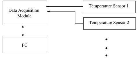
Figure 1 shows the block diagram of the temperature monitoring system. The main components are the data ac-quisition (DAQ) device and the temperature sensor. Power to the temperature sensor is provided by the DAQ device as well.
0 1 0 0 1 1 0 0 1 1 0000000000
1111111111 Temperature Sensor 1
Module Data Acquisition
PC
[image:1.595.307.543.583.683.2]Temperature Sensor 2
Fig. 1. System Block Diagram
be used which would trade additional development time for lower cost.
The DAQ has 32 input channels which is enough for both phase one and phase two activities. The DAQ inputs are configured to sense voltages between 0 to 2 volts in anticipation of the temperature sensor output between 0 to 1 volt.
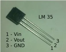
[image:2.595.111.226.199.290.2]The temperature sensor to be used is the popular three-terminal LM35 sensor [7]. As shown in Figure 2, the device has three terminals, namely, voltage input (Vin), voltage output (Vout) and ground (GND).
Fig. 2. LM35 Temperature Sensor
For minimal component count operation, all that is needed is to apply voltage (5V) between the voltage input and ground terminals. The voltage output terminal (referenced to ground) will then return a voltage proportional to temperature at a ratio of 10 mV/C. However, due to the multiplexing operation of the DAQ, it was necessary to connect a dummy resistive load between output terminal and ground of the LM35 sensor in order to get reliable and consistent voltage readings.
Since the LM35 sensor is not exactly designed to be embedded in concrete, additional preparations were made to electrically isolate the terminals while still maintaining direct contact as much as possible between the sensor casing and the surrounding concrete. The goal is to avoid electrical interaction with the concrete without compromising thermal interface. Heatshrink tubings were placed around the three terminals to avoid an electrical short. After which, the sensors were dipped in epoxy to further seal the electrical contacts from any liquid. Finally, a portion of the casing and whole terminals were encapsulated with heatshrink tubing.
For the laboratory phase of this project, a concrete mold 30.5 cm high and 15.2 cm diameter made of steel similar to that shown in [8] is used for the test setup.
Two temperature sensors were fastened to a round steel bar and positioned at the center of the mold. Concrete is then poured into the mold while temperature is monitored. For reference, the room temperature was also monitored using another temperature sensor.
B. DAQ Setup
The immediate goal for phase one was to test the func-tionality of the whole setup from the DAQ to the sensors. With only three sensors to read and store the data, no issue was encountered with the DAQ configured for the fastest acquisition time.
In preparation for phase two, a sample run where all 32 sensors were read and then stored was performed. However, considering that the field run for phase two would last for days and that 32 sensors will be read, sampling at the
fastest rate would mean a voluminous amount of data will be gathered which may lead to storage issues for the host computer.
It was then decided that a sampling rate of 0.1 Hz will be acceptable since it is not expected that temperature will be changing quickly. However, the NI DAQ default configuration for sampling was inflexible. If a sampling rate of 0.1 Hz was set, it was expected that we will receiving 32 readings from the 32 sensors every 10 seconds. Due to how the NI DAQ operates by default, a 0.1 Hz sampling would indeed give 32 readings after every 10 seconds. However, the 32 readings would not be gathered all at same time as would be expected but gathered one at a time after every 0.312 seconds. To rectify this issue, the NI DAQ was custom programmed to acquire the 32 consecutive sensor readings as close in time as possible to each other while reporting all the samples every 10 seconds. This DAQ configuration was necessary to ensure that the sensor events being recorded are more or less happening at the same time instead of being spread out across ten seconds.
C. Phase Two. Field Testing
The second phase involves field testing of the setup. The same basic setup is used as shown in Figure 1. However, 32 sensors are now connected to DAQ. The same preparations as in phase one were made to each of the 32 LM35 temperature sensors.
The setup will be deployed in a dam construction site where concrete is scheduled to poured. The sensors will be arranged about a 5 m x 10 m area as shown by the black dots in Figure 3.
0 0 1 1 0 0 1 1 0 0 1 1 0 0 0 1 1 1 00 00 11 11 0 0 1 1 0 0 1 1 0 0 1 1 0 0 1 1 0 0 1 1 000000 000000 000000 000000 000000 000000 000000 000000 000000 000000 000000 000000 000000 000000 000000 000000 111111 111111 111111 111111 111111 111111 111111 111111 111111 111111 111111 111111 111111 111111 111111 111111 0 0 1 1 0 0 1 1 0 0 1 1 0 0 0 1 1 1 00 00 11 11 0 0 1 1 0 0 1 1 0 0 1 1 0 0 1 1 0 0 1 1 000000 000000 000000 000000 000000 000000 000000 000000 000000 000000 000000 000000 000000 000000 000000 111111 111111 111111 111111 111111 111111 111111 111111 111111 111111 111111 111111 111111 111111 111111 0 0 1 1 0 0 1 1 0 0 1 1 0 0 0 1 1 1 00 00 11 11 0 0 1 1 0 0 1 1 0 0 1 1 0 0 1 1 0 0 1 1 000000 000000 000000 000000 000000 000000 000000 000000 000000 000000 000000 000000 000000 000000 000000 000000 111111 111111 111111 111111 111111 111111 111111 111111 111111 111111 111111 111111 111111 111111 111111 1111110 0 1 1 0 0 1 1 0 0 1 1 0 0 0 1 1 1 0000000000000000 0000000000000000 0000000000000000 0000000000000000 0000000000000000 0000000000000000 0000000000000000 0000000000000000 0000000000000000 0000000000000000 0000000000000000 0000000000000000 0000000000000000 0000000000000000 0000000000000000 0000000000000000 0000000000000000 0000000000000000 0000000000000000 1111111111111111 1111111111111111 1111111111111111 1111111111111111 1111111111111111 1111111111111111 1111111111111111 1111111111111111 1111111111111111 1111111111111111 1111111111111111 1111111111111111 1111111111111111 1111111111111111 1111111111111111 1111111111111111 1111111111111111 1111111111111111 1111111111111111 00 00 00 11 11 11 000 000 111 111 0000000000 0000000000 0000000000 0000000000 0000000000 0000000000 0000000000 0000000000 0000000000 0000000000 1111111111 1111111111 1111111111 1111111111 1111111111 1111111111 1111111111 1111111111 1111111111 1111111111 0 0 0 1 1 1 0 0 1 1 0 0 0 0 0 0 0 0 0 0 0 0 1 1 1 1 1 1 1 1 1 1 1 1 10m 3m 5m
Fig. 3. Sensor Locations
The sensors will be fastened to round steel bars especially set up for this experiment as shown Figure 4. Concrete pour will be to a height of two to three meters.
III. RESULTS ANDANALYSIS
[image:2.595.307.543.448.589.2]Fig. 4. Mounting Frame for Sensors
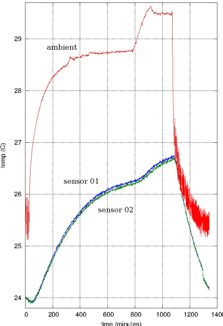
Fig. 5. Laboratory Setup Results
temperature by the concrete temperature sensors. As can be seen from the temperature readings inside the concrete, we can conclude that the temperature sensors survived the pouring process and the curing process.
For the field test, data was gathered for seven days. The data acquired can be classified into the following categories, namely, success, partial success and fail. The data collected for a particular sensor is categorized as a success if no readings went beyond 1.05 volts (or 105 C). Readings are a partial success if a small subset of the readings went beyond the 1.05 volts limit but not enough to make the whole set unusable. In case of partial success, trends can still be
identified from the readings. The data collected is considered fail if most of the readings went beyond the limit which makes the data unusable for tracking temperature.
Readings for 18 sensors were considered a success. Figure 6 shows the plots of all the sensor readings considered a success.
te
m
p
er
at
u
re
(C
)
time (days) 20
30 40 50 60 70 80
0 1 2 3 4 5 6 7
Fig. 6. Field Result, Success Readings
It can be seen from Figure 6 that temperature readings are within the expected range. Depending on the sensor location, temperatures can peak as high as 72 degrees Celsius. The plots also show that temperatures start out near ambient and increases after the concrete is poured. Peak temperatures are then reached between one or two days after the pouring and then steadily decreases. Some spikes in the temperature readings can be observed for two of the sensors. This may indicate that the particular sensors are borderline functional. Figure 7 shows plots of partial success readings. The two sensor readings from sensor 02 and sensor 06 shown in the graph all have readings beyond the 1.05 volts limit. The readings for sensor 02 are nearly successful readings. The readings from both sensors still show the temperature trends.
100 120
te
m
p
er
at
u
re
(C
)
time (days) 20
40 60 80
0 1 2 3 4 5 6 7
[image:3.595.54.282.260.592.2]sensor 02 sensor 06
Fig. 7. Field Result, Partial Success Readings
[image:3.595.312.538.552.730.2]Similar to readings from sensor 02 shown in Figure 7, the readings from sensor 23 are nearly successful readings with a few glitches found around the first day and towards the end.
100 120
te
m
p
er
at
u
re
(C
)
time (days) 20
40 60 80
0 1 2 3 4 5 6 7
[image:4.595.313.536.63.241.2]sensor 23
[image:4.595.58.279.124.302.2]Fig. 8. Field Result, Partial Success Readings from Sensor 23
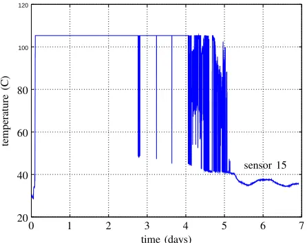
Figure 9 are plots for readings that can still be considered partial success. Although the readings are certainly far from being a success, temperatures and trends can still be inferred. And if, for example, one is only interested in the final temperature after seven days, then sensor 15 data can be used.
100 120
te
m
p
er
at
u
re
(C
)
time (days) 20
40 60 80
0 1 2 3 4 5 6 7
[image:4.595.329.523.354.442.2]sensor 15
Fig. 9. Field Result, Partial Success Readings from Sensor 15
The Figures 11 and 12 found in the appendix shows two additional readings from sensor 07 and sensor 27, respectively. Similar to the readings from sensor 15, trends can still be inferred from those readings. They may still be used for determining the temperature during some periods.
Figure 10 shows the plots of the readings for sensors that have been considered to have failed. The readings show no discernable pattern that can be used for determining the temperature. Most of the readings are at the 1.05 volts limit for these cases. Another set of plots for readings that are classified as failed are found in the appendix in Figure /reffig:fail1222.
100 120
te
m
p
er
at
u
re
(C
)
time (days) 20
40 60 80
0 1 2 3 4 5 6 7
sensor 10 sensor 17
Fig. 10. Field Result, Fail Readings
Based on the above classification of readings, Table I shows the sensors under each classification and the total sensors that are either a success, partial success or fail.
TABLE I
SENSORFUNCTIONALITYSUMMARY
Classification Sensor Number Total 03, 04, 08, 09, 11, 13,
Success 14, 16, 19, 20, 21, 24, 18 25, 26, 28, 30, 31, 32
Partial 02, 06, 07, 15, 23, 27 6 success
Fail 01, 05, 10, 12, 17, 18, 22, 29 8
It can be seen that most of the sensors survived the pouring and curing process, and were able to give acceptable readings.
IV. CONCLUSIONS ANDFUTUREWORK
In conclusion, we see that the LM35 temperature sensor can be embedded in concrete and used to sense internal temperature of the curing concrete. The lab experiment show that for small volumes of concrete, there was no issue embedding the sensor. The two sensors survived the process. For the field test with 32 sensors, we see that a significant number of sensors were functional and usable for tracking the internal temperature of concrete. We did see some sensors failing, most probably due to exposure to the concrete. With the low cost of the LM35 sensor, several devices can be simultaneously embedded which increases the reliability of getting temperature readings.
For future work, a more robust encapsulation of the sensor can be used. Instead of using heatshrink tubings, copper tubings can be used. Further studies can be made whether the failure of sensor was caused by an electrical issue due to the exposure to the concrete or a mechanical stress to the sensor when the concrete was curing.
APPENDIXA
ADDITIONALFIELDRESULTSREADINGS
[image:4.595.57.280.430.607.2]for partial success readings while Figure 13 are for fail readings.
100 120
te
m
p
er
at
u
re
(C
)
time (days) 20
40 60 80
0 1 2 3 4 5 6 7
[image:5.595.57.279.104.280.2]sensor 07
Fig. 11. Field Result, Partial Success Readings from Sensor 07
100 120
te
m
p
er
at
u
re
(C
)
time (days) 20
40 60 80
0 1 2 3 4 5 6 7
[image:5.595.58.279.339.516.2]sensor 27
Fig. 12. Field Result, Partial Success Readings from Sensor 27
100 120
te
m
p
er
at
u
re
(C
)
time (days) 20
40 60 80
0 1 2 3 4 5 6 7
sensor 12
sensor 22
Fig. 13. Field Result, Fail Readings from Sensors 12 and 22
ACKNOWLEDGMENT
This research was done in collaboration with Dr. Nathaniel B. Diola, Associate Professor of the Institute of Civil En-gineering and Director of the Building Research Service, University of the Philippines.
REFERENCES
[1] Carino, N., ”The Maturity Method: Theory and Application,”Cement, Concrete and Aggregates, Vol. 6, No. 2, pp. 61-73, 1984.
[2] Bofang, Z., Thermal Stresses and Temperature Control of Mass Concrete, 1st Edition, Butterworth-Heinemann, November 14, 2013. [3] SmartRock2 Temperature/Maturity Sensor,
http://www.giatecscientific.com/product/giatec-smartrock/english-smartrock/
[4] IntelliRock Wireless System, http://www.engius.com/web/products/ir-wireless.asp
[5] Norrisa A., Saafib M., Rominec P. ”Temperature and Moisture Monitoring in Concrete Structures Using Embedded Nanotechnol-ogy/Microelectromechanical Systems (MEMS) Sensors,”Construction and Building Materials, Vol. 22, Issue 2, pp. 111120, February 2008. [6] Barroca N., Borges L., Velez F., Monteiro F. Grski M., Castro-Gomes J., ”Wireless Sensor Networks for Temperature and Humidity Monitoring within Concrete Structures,” Construction and Building Materials, Vol. 40, pp. 1156 - 1166, 2013.
[7] ”LM35 Precision Centigrade Temperature Sensors,” http://www.ti.com/product/LM35/datasheet.
[image:5.595.58.279.573.751.2]