Abstract—We present a mathematical model which describes the development of coinfection with HBV (Hepatitis B virus) and HCV (Hepatitis C virus), in a patient in a “congested” environment. We assume that, while susceptible patients become infected with HBV and/or HCV through physical contact (sexual, sharing needles, and so on), coinfection occurs simply because they live in close proximity to each other, a situation which is true in densely populated situations like penitentiaries, refugee camps, etc., and sometimes in overpopulated countries. A similar assumption about coinfection with HCV and HIV (human immunodeficiency virus) has also been made by other researchers. We shall, accordingly, assume that a certain percentage of people who are infected with HBV in a densely populated environment are also co-infected with HCV, and vice versa. We give several examples to illustrate the behavior of the model.
Index Terms—basic reproduction ratio, co-infection, congested environment, Hepatitis B virus, Hepatitis C virus, mathematical modeling
I. INTRODUCTION
NE hundred and seventy million people are infected with
HCV (Hepatitis C virus) worldwide [1, 2]. In North America, more than five million people are estimated to be living with HCV [2, 3]. Approximately 30,000 new cases are diagnosed each year, and this situation is projected to get worse as the number of people infected with HCV from blood transfusions before 1990 come to be newly diagnosed [2]. This is because, before 1990, there was no screening of blood against HCV (HCV was discovered in 1989), so that millions of patients must have been infected through blood transfusions. These cases are now coming to light because the disease can stay asymptomatic for 20 years and more. Historically, the disease is speculated to have been brought into the United States from West Africa at the time of the slave trade [2]. Today, it kills more people than HIV (human immunodeficiency virus) every year in that country. In some countries in Africa, like in Egypt, the virus affects almost one in every five adults. If untreated, HCV results in generally fatal liver failure. If treated, the treatment is unsuccessful in over half of the patients. Like HIV, HCV can stay dormant for years while attacking the liver all this time. HCV mutates easily which makes for a large number of mutant viruses (and makes the development of a vaccine that much more difficult). There are six known genotypes (numbered 1 through 6) and more than 50 subtypes (e.g., 1a, 1b, 2a ...). These genotypes and their subtypes are present in different proportions in different countries. As an example, genotype
Manuscript received May 25, 2016.
B. D. Aggarwala is a professor emeritus at the University of Calgary, Canada. (email: [email protected])
1 is the dominant type in the United States, while in India, genotype 3 seems to be more prevalent [4].
The history of HBV (Hepatitis B virus) goes back to the 1950' s when a Dr. Baruch Blumberg was taking samples from the blood of aborigines in Australia. Dr. Blumberg was interested in polymorphism and he wanted to see whether inherited traits could make different people more or less susceptible to infection by certain viruses. During these trials, he tested the blood of several hemophiliacs because these people were routinely exposed to different kinds of blood through blood transfusions, and the immune system of the recipient should produce antibodies against the antigens in the donors’ blood. In 1963, Dr. Blumberg identified an antigen that detected the presence of Hepatitis in the blood samples. That virus was officially recognized as HBV in 1967 and a vaccine for the virus was discovered in 1969 [5]. Today, more than 240 million people are chronically infected with the virus [6], mainly because, in many countries, vaccination is not followed thoroughly enough. In Southeast Asian countries for example, approximately 5 - 10% of the population are carriers of HBV, while in North America and Europe, this figure is about 0.5 % because of better vaccination practices. In Canada, the incidence of reported HBV infection has dropped dramatically after 1995. It was estimated at 2.3/100,000 in 1998 [7]. Dr. Blumberg received a Nobel Prize for his work in 1876.
While HCV infection can be cured, and the virus can re-infect, chronic HBV generally ends up in hepatocellular carcinoma (liver cancer). Almost 90 percent of babies and about 5 - 10% of adults who contract HBV develop the chronic form of it and may need liver transplant [7]. However, the chance of the virus being reactivated after liver transplant is also quite high. Overall, we may say that a certain percentage of people who get infected with HCV or HBV and get cured, get sick again with the same infection.
In many developing countries, with very high population densities, co-infection with both HBV and HCV is fairly common [8, 9, 10, 11]. According to one writer, “HCV superinfection in patients with chronic HBV infection was the most common clinical feature of coinfection in Asia–Pacific countries” [10]. This is perhaps because of over population in these countries. In such situations, people live in close proximity and generally, are not well cared for. Medical facilities are minimal, and these facilities are generally availed of only when the patients are seriously sick, which in the context of this paper, means when they are co-infected. Also, people who are already infected with HBV or HCV, are
On a Mathematical Model for HBV and HCV
Co-infection
B. D. Aggarwala, Member, IAENG
likely to have similar "risky" behavior (risk factors for both HBV and HCV are the same), so that contacts are fairly common (social, sexual, sharing needles and other), which facilitates coinfection. Considering all this, one may assume that a certain fraction of people, living in “congested situations” and suffering from HBV are also suffering from HCV and vice versa. Such considerations (about congestion) are applicable in many situations like penitentiaries, refugee camps, slums in big cities (Dharavi in Mumbai?) and so on.
We present a mathematical model which describes the development of coinfection with HBV and HCV, in a patient in a congested environment. We assume that, while patients become infected with HBV and/or HCV through physical contact (sexual, sharing needles, and so on) coinfection occurs simply because they live in close proximity to each other, a situation which is true in densely populated situations like penitentiaries, refugee camps, etc. A similar assumption about coinfection with HCV and HIV has also been made by other researchers [12]. We shall, therefore, assume that a certain percentage of people who are infected with HBV in a densely populated environment are also co-infected with HCV, and vice versa. We give several examples to illustrate the behavior of the model. However, these examples are not specific to HBV/HCV coinfection but simply to illustrate how the model behaves under such conditions.
II. THE MODEL
A. Set Up
We write
4 12 4 11 4 10 3 9 2 8 4 3 2 1 4 4 12 3 7 4 1 5 1 3 1 4 4 3 2 1 3 4 11 2 6 4 1 5 1 2 1 3 4 3 2 1 2 4 1 5 3 1 4 2 1 3 1 2 1 4 3 2 1 1 , , , 1 , , , , , , , , , x A x A x A x A x A x x x x F x A x A x x A x x A x x x x F x A x A x x A x x A x x x x F x x A x x A x x A x A A x x x x F with x1'F1,x2'F2,x3'F3, and x4'F4.
All the parametersA1,A2,... etc. are supposed to be non-negative.
In these equations,x1,x2,x3and x4refer to the number of
susceptible people, people infected with HBV, those infected with HCV, and those who are co-infected, respectively. Susceptible people become infected with HBV and/or HCV when they come into contact with similarly infected people according to the termsA3x1x2andA4x1x3. If a susceptible
person(x1)comes into contact with a co-infected person )
(x4 , then he/she becomes infected with either HBV or HCV
(but not both) according to the terms1A5x1x4and
11
A5x1x4, so that a certain percentage of people (0 < 1< 1) become infected with HBV and others with HCV (but not both). Also, a certain percentage of people who are infected with HBV (or HCV) also get co-infected (according
to the termsA8x2,andA9x3)because of congested
environments, and also because the risk factors for both infections are the same. Some of these co-infected people
) ,
(A11x4 A12x4 get cured, mostly through medical
intervention, of either HBV or HCV (but not both) and become candidates for reinfection by that virus. We ignore the very small number of co-infected people who get cured of both the infections, and rejoin thex1class.
B. Positivity of the Solution
It is clear that, in the beginning, when the disease strikes,
1
x is close to its equilibrium value of A1/A2, x2and x3 are
close to one, andx4is zero, so that we are starting in the
non-negative space, namely in x10,x20,x30, andx4 0.
Now we write x
x1,x2,x3,x4
. Now notice that we can write our equations as x'F(x)V(x)whereF(x)and) (x
V are appropriate vector functions. The function F(x) stands for all the 'positive' terms andV(x)for all the 'negative' ones in (1a) to (1d), so that
} ) ( , , , { ) ( 4 12 11 10 3 7 2 6 4 1 5 3 1 4 2 1 3 1 2 x A A A x A x A x x A x x A x x A x A x V
andF(x)represents all the remaining terms. Now if the "particle" "x" starts in the non-negative space
, 0 , 0 , 0
(x1 x2 x3 andx4 0),and follows the path
), ( ) (
' F x V x
x then it cannot go into the negative space because ofF(x)(because all these terms are positive and we started in the positive space). Also if xi = 0 {i = 1, 2, 3, 4}, then the corresponding component of V(x) is also zero, and
) (x
V is a polynomial, so that this particle cannot go into negative space because of V(x)either. Since the initial conditions placed the particle x
x1,x2,x3,x4
in thenon-negative space, it is bound to stay in that space.
This proves the invariance of the non-negative space for the solutions of our model. In light of this result, (and since the initial conditions in our investigations will always be in the non - negative space), if there are any solutions of our equations (numerical or otherwise) with negative components, we shall call them irrelevant (or unviable, or non-reachable) solutions. In what follows, we shall prove the important result that there is at most one viable solution of our equations other than the disease free one.
C. Boundedness of the Solution
We have . )' ( 4 10 3 9 3 7 2 8 2 6 1 2 1 4 3 2 1 x A x A x A x A x A x A A x x x x
Since A7 > A9 and A6 > A8 (A6x2 and A7x3 represent the
number of people who get co-infected, plus those who die), the right hand side is clearly negative for A2x1 + A6x2 - A8x2 +
A7x3 - A9x3 + A10x4 > A1. Also this quantity is clearly positive
for A2x1 + A6x2 - A8x2 + A7x3 - A9x3 + A10x4 < A1. It follows that
a particle starting in {x1, x2, x3, x4} ≥ {0, 0, 0, 0} will approach
the (bounded) region A2x1 + A6x2 - A8x2 + A7x3 - A9x3 + A10x4 =
A1 and stay there. All the equilibrium points of the system
(1a)
(1b)
(1c)
Fi[x1, x2, x3, x4] = 0, i = 1, 2, 3, 4 must be located in this region.
The point {x1, x2, x3, x4} = {A1/A2, 0, 0, 0} is an example (the reader may verify for other solutions in this paper).
D. Equilibrium Points
The equilibrium points of our system can best be found by eliminating x1, x2, x3, and/or x4 successively from the
equations. Eliminating x2 from F1 = F2 = F3 = F4 = 0, for
example, we get L2 = 0, where, apart from the root x2 = 0, L2
= 0 is a second degree equation like + + = 0, where the terms A, B, and C are too long to reproduce here. This equation has two roots. We shall call them x21 and x22.
Similarly for (x11 and x12), (x31 and x32) and (x41 and x42). We
find
(x21x22) / (x41x42) = {A11(A10 + A11 + A12)A4 + A11A5A9 +
A5[A10A7 + (A11 + A12) (A7 - A9)]θ1} / [(A4A6
- A3A7)A8];
(x31x32) / (x41x42) = -{1/[(A4A6 - A3A7)A9]}{A10A12A3 +
A11A12A3 + (A12)2A3 + A10A5A6 + A11A5A6 +
A12A5A6 - A11A5A8 - A5[A10A6 + (A11 + A12)
(A6 - A8)]θ1},
and
(x21x22) / (x31x32) = {-A11A9[(A10 + A11 + A12)A4 + A5A9]
+ A5A9[-(A10+A11+A12)A7 + (A11 + A12)A9]θ1}
/ {A8[A10A12A3+A11A12A3+(A12)2A3 + A10A5A6
+ A11A5A6 + A12A5A6 - A11A5A8 - A5(A10A6 +
{A11 + A12}{A6 - A8})θ1]}.
Under the assumptions that A6 > A8 and A7 > A9 (notice that
A6 and A7 represent the number of people who get co-infected
plus those who die), it is easily seen that the quantity (x21x22)
/ (x31x32) is negative. This says that either x21x22 is negative
(which requires either x21 or x22 to be negative) or that x31x32 is
negative, while the other number is positive. In either case, we must discard one of the two solutions, (x11, x21, x31, x41) if
x21 is negative and (x12, x22, x32, x42) if x22 is negative. Similarly
for x31x32. We are now left with only one viable solution (other
than the disease free one) of our equations.
E. Basic Reproduction Ratio
The basic reproduction ratio of such a dynamic is a measure that indicates whether the disease will grow or die out. This number has been termed "the most significant contribution of Mathematics to Epidemiology" [13]. If, when ALL the people are susceptible, i.e. in the beginning when the disease strikes, one infected person infects MORE THAN ONE person in his/her (infectious) lifetime, then obviously the disease will spread (because one becomes two, two becomes four and so on), while if one person infects LESS THAN ONE person, then the disease will die out (because now four becomes two, two becomes one and so on). An elementary example for illustration of this idea is the equation
x' = ax - bx, where x = 0 is the uninfected state. If in the beginning when x = ε > 0 (the disease strikes) then, if a > b, the x values go to infinity, while if a < b, the x values go to zero. Since x = 0 is the point of equilibrium in this case, it follows that this point of equilibrium is stable if a / b < 1 and
is unstable if a / b > 1. In the latter case, the disease spreads while in the former caser, it dies out. The terms ax and bx may be called the incoming and outgoing terms (to x') respectively. The Basic Reproduction Ratio R in this case is
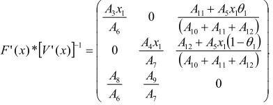
a / b. The disease spreads if R > 1 and dies out if R < 1. In the above analogy (x' = F(x) - V(x)), we have F(x) = ax and V(x) = bx. If F '(x) / V'(x) > 1, the disease spreads, and the x values increase, i.e. the equilibrium value (x = 0) is unstable, while if F '(x) / V '(x) < 1, the equilibrium value (x = 0) is stable and the disease dies out. The quantity F '(x) / V '(x) is the BASIC REPRODUCTION RATIO (R0) of this dynamic. If the number of equations in the dynamic is more than one, this ratio is replaced by a (very similar looking) ratio. Now F(x) and V(x) become appropriate matrices (of incoming and outgoing terms respectively), x represents an appropriate vector, F '[x] and V '[x] are matrices with components Fi (xj) and Vi (xj), and the basic reproduction number (which is a ratio) is the (largest) eigenvalue of the matrix, F '[x] / [V '[x]], (or, more appropriate in this setting, of F '[x]*[V '[x]]-1). This ratio is calculated at the point where the state of the system is uninfected (see [14,15] for details).
It is not clear as to how we should calculate this number in the case of co-infection/re-infection. Generally, the way to calculate R0 is that "Once an individual is diagnosed, his/her contacts are traced and tested. R0 is then computed by averaging over the number of secondary cases of many diagnosed individuals" [16]. So, what is a secondary case? If the susceptible people are infected and then get co-infected with HBV and/or HCV, and get re-infected (or reactivated) after getting cured, how should we count as to how many infected people a susceptible person originally produces? What are F(x) and V(x) for this situation? Is there a unique
R0 in this case? If this reinfection and/or coinfection did not occur, would it not affect the total number of infected people and consequently, the basic reproduction ratio? It has been shown in the context of a different ailment (TB) that re-infection does change the Basic Reproduction Ratio [17]. Our results in this paper indicate that if R0 is computed by "averaging over the number of secondary cases of many secondary individuals" which are co-infected or re-infected, then you are likely to "underestimate" the true value of R0 in the important case when the disease is endemic.
If {x2, x3, x4} = {0, 0, 0} is the uninfected state, should we
take all entries into this state as the incoming terms or only those that involve x1? We try to answer this question for our
model below by considering various cases. In our examples, we take {x2, x3, x4} = {0, 0, 0} as the uninfected state.
1) Case One:
From (1b) – (1d), we take the incoming and outgoing terms as
F(x) = {{A3x1x2 + 1A5x1x4}, {A4x1x3 + (1-1)A5x1x4}, {0}};
V(x) = {{A6x2 - A11x4}, {A7x3 - A12x4}, {A10x4 + A11x4 + A12x4
- A8x2 - A9x3}}.
F’(x) = {{A3x1,0,1A5x1}, {0,A4x1,(1-1)A5x1}, {0,0,0}};
V’(x) = {{A6,0,-A11}, {0,A7,-A12}, {-A8,-A9, A10+A11+A12}}. The basic reproduction ratio, R0, is the spectral radius of
F’(x)*[V’(x)]-1 [9]. However, this matrix has three eigenvalues, let us call them R0, R00, and R000. The largest of
these eigenvalues is R0 where
R0 = {A10A4A6x1 + A11A4A6x1 + A12A4A6x1 + A10A3A7x1 +
A11A3A7x1 + A12A3A7x1 - A11A4A8x1 - A12A3A9x1 +
A5A6A9x1 + A5A7A8x11 - A5A6A9x11 + sqrt[(-A10A4A6x1
- A11A4A6x1 - A12A4A6x1 - A10A3A7x1 - A11A3A7x1 -
A12A3A7x1 + A11A4A8x1 + A12A3A9x1 - A5A6A9x1 -
A5A7A8x11+ A5A6A9x11)2 – 4*(A10A6A7+ A11A6A7+
A12A6A7 - A11A7A8 - A12A6A9)(A10A3A4x12 + A11A3A4x12
+ A12A3A4x12 + A3A5A9x12 + A4A5A8x121 -
A3A5A9x121)]} / [2*(A10A6A7+ A11A6A7+ A12A6A7-
A11A7A8 - A12A6A9)].
Note: It should be noticed that if {x11, x21, x31, x41} is the
(only) viable solution, then the basic reproduction ratio of our dynamic may also be written as A1 / (A2x11). This is because,
at the point of equilibrium, each newly infected person must exactly replace him/herself, i.e. produce one new infected person in his/her (infectious) lifetime, (this is what equilibrium should mean). The number of infected persons that one infected person produces (in his/her infectious lifetime) clearly depends upon the number of susceptible persons that the infected person interacts with. If an infected person interacts with 100 people and produces one infected person say, then if that person interacts with 200 people, s/he will produce two infected persons (on the average). So, if the susceptible number of persons is A1 / A2 in the beginning and
interaction with these people produces R infected people say, then the susceptible number of persons at the point of equilibrium (when one infected person produces exactly one infected person), must be 1/R times the original number of persons. It follows that
x11 = A1 / (A2R) or R = A1 / (A2x11) (2)
It is now clear that, if we have an independent expression for x11 in our model we can get another expression for R (we
shall call this expression R1). Such an expression for x11 can
be obtained by eliminating x2, x3 and x4 from the equations in
our model. The result of this elimination is [x1 - (A1 / A2)] L1
= 0 where L1 is a second degree polynomial of the type Ax12
+ Bx1 + C. The smaller of the two roots of L1 turns out to be
x11 (corresponding to the larger value of R), while the larger
of these two roots corresponds to the other smaller eigenvalue. (The root x1= A1/ A2 of the original equation
corresponds to the infection free equilibrium value of x1). We
get
x11 = {A10A4A6 + A11A4A6 + A12A4A6 + A10A3A7 + A11A3A7 +
A12A3A7 - A11A4A8 - A12A3A9 + A5A6A9 + A5A7A81 -
A5A6A91 - sqrt[-4*(A10A6A7 + A11A6A7 + A12A6A7 -
A11A7A8 - A12A6A9)(A10A3A4 + A11A3A4 + A12A3A4 +
A3A5A9 + A4A5A81 - A3A5A91) + (-A10A4A6 - A11A4A6
- A12A4A6 - A10A3A7 - A11A3A7 - A12A3A7 + A11A4A8 +
A12A3A9 - A5A6A9 - A5A7A81 + A5A6A91)2]} /
[2*(A10A3A4 + A11A3A4 + A12A3A4 + A3A5A9 + A4A5A81
- A3A5A91)],
and then R1 = A1 / A2x11. As we pointed out above, the basic
reproduction ratio is also the spectral radius of an appropriate matrix. Each eigenvalue of this matrix corresponds to an equilibrium value (stable or otherwise) of x1. Since the
spectral radius refers to the (numerically) largest eigenvalue of a matrix, the corresponding value of x11 should be the
minimum of all such values. This explains the minus sign before the square root sign in the above expression.
a) Example 1
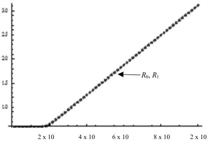
As an example, we show the values of R0 and R1 = A1 / A2x11
for some values of the parameters. Notice that they are coincident (there is a continuous line under the dots in Fig. 1). We take A1 = 1; A2 = A1/15,000; A4 = 0.9A3; A5 = 0.9A3; 1
= 0.5; 2 = 1 - 1; A6 = 1/2000; A7 = 0.5A6; A9 = 0.0002; A8 =
A9; A10 = 0.01; A11 = 0.1A10; A12 = A11; x1 = A1/A2,
and calculate the values of these two quantities for some values of A3:
[image:4.612.322.529.322.465.2]
Fig. 1. Values of Basic Reproduction Ratio (as Ro and R1) against values of
A3, calculated two different ways (1) as A1/A2x11 and (2) as the largest eigenvalue of an appropriate matrix. Notice that they are coincident. (Notice the continuous line under the dots).
b) Example 2
As another example, we take A1 = 1; A2 = A1/10,000; A3 =
0.0000001; A4 = 0.5A3; A5 = 0.5A3; 1 = 0.9; 2 = 1 - 1; A6 =
1/2000; A7 = A6; A9 = 0.0002; A8 = A9; A10 = 0.001; A11 = 0.3A10;
A12 = A11.
At x1 = A1/A2we get
{R00, R0} = {1.07713, 2.33463},
where R00 is another eigenvalue of our matrix. The spectral
radius turns out to be 2.33463 and we should get one (and only one) viable solution. Solving (1a) – (1d) in the software
Mathematica we get:
{x1, x2, x3, x4} = {10,000, 0, 0, 0}, {9283.92, -35.288,
203.776, 21.061} or {4283.33, 1156.03, 189.069, 168.137}.
The last one is the viable solution. Notice that although two 2 x 10⁻⁸ 4 x 10⁻⁸ 6 x 10⁻⁸ 8 x 10⁻⁸ 2 x 10⁻⁷
values of R are greater than one, there is only one viable solution as our analysis argues. Notice this value corresponds with the smaller of the two equilibrium values of x1. Also
notice that A1 / A2*4283.33 = 2.33463, and A1 / A2*9283.92 =
1.07713, which is the other value R.
Every eigenvalue of the matrix F’(x)*[V’(x)]-1 corresponds to an equilibrium value of x1 (stable or otherwise) in our
solution, the largest eigenvalue corresponding to the only viable solution. Numerically graphing the solution using
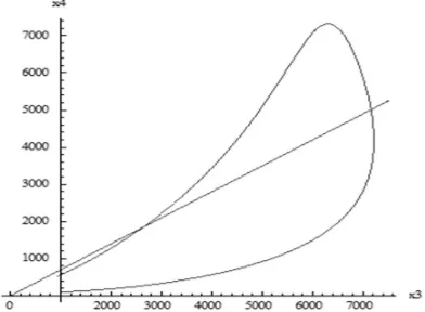
Mathematica, we see the distribution of HCV and HBV infected people in the population in Figs. 2 and 3. It should be noted that the number of HCV infected people is between approximately 3% and 20% of those who are HBV infected (approximate slopes of the two bounding straight lines in Fig. 2). The number of co-infected people (x4) amongst the HCV
infected ones (x3) is given in Fig. 3. This number is close to
70% (slope of the straight line).
10,000 20,000 30,000 40,000 50,000 60,000 70,000
[image:5.612.84.289.254.400.2]x2
Fig. 2. Number of HBV infected people (x2, along the horizontal axis) as against the co-infected ones (x4) in this example. This number of co-infected ones falls between approximately 3% and 20% of HBV infected ones (approximate slopes of the two bounding straight lines). In surveys, these rates vary from 9% to 30% [18]. The number of co-infected people rises in the beginning but soon recoils back, so that any time you take a sample, this ratio will be close to 10%.
Fig. 3. Number of co-infected people (x4) amongst the HCV infected ones (x3) in this example. The number of HCV infected people rises in the beginning but soon recoils back, so that any time you take a sample, this ratio will be close to 70% (slope of the straight line).
Note: It may happen that x21 and x22 (or x31 and x32) are both
negative, (for x21x22 or x31x32 to be positive). In this case both
the solutions {x11, x21, x31, x41} and {x12, x22, x32, x42} must be
discarded and we are left with NO viable solution. Similarly for x31x32. This should happen when the basic reproduction
ratio is less than one, as in the following example.
c) Example 3
We take A1 = 1; A2 = A1/1000; A3 = 0.0000001; A4 = 0.9A3;
A5 = 0.5A3; 1= 0.5; 2 = 1 - 1; A6 = 1/2000; A7 = A6; A9 =
0.0002; A8 = A9; A10 = 0.001; A11 = 0.5A10; A12 = 0.5A11.
Solving (1a)-1(d), we get:
{x1, x2, x3, x4} = {5385.92, 19,896.9, -30,483.6, -1209.91} or
{1000, 0, 0, 0} or {4030.24, 5178.52, -2135.87, -835.929}. Notice that there is no viable solution other than the disease-free one. Also, in this case at x1 = A1/A2 we get
{R00, R0} = A1/A2x1= {0.185669, 0.248124},
which says that both roots are less than one.
Basic Reproduction Ratio Again: We stated above that "If an infected person interacts with 100 susceptible people and produces one infected person say, then, if that person interacts with 200 susceptible people, s/he will produce two infected persons (on the average)." It is not clear whether such a linear relationship will be true if the infected people recover from their ailment and start getting infected again. In the case of ODE models in epidemiology, it is particularly difficult to calculate this number (the basic reproduction ratio) from the model [19]. In the case of the model mentioned above, namely x'(t) = ax - bx, if we write the same equation as x'(t) = (a + n)x - (b + n)x, for any number n > 0, would the new estimate of this ratio be (a + n) / (b + n), which is different from a / b? The obvious conclusion is that we cannot estimate this ratio from the mathematical model itself. However, notice that both these numbers a / b and (a + n) / (b + n) correctly predict the regime where the (infected) population will grow or will shrink, i.e. if a / b > 1, a / b = 1, or a / b < 1, then so is (a + n) / (b + n) for any positive number n. A similar conclusion has been reached by other researchers in the field [19]. We shall now give a number of scenarios where an approximate ratio (R) for our model is calculated differently each time.
2) Case two
In analogy with the above example about ((a+n)/(b+n)), we shall take various forms of the incoming and outgoing functions F(x) and V(x) and calculate the corresponding R. In our model, we take {x2, x3, x4} = {0, 0, 0} as the uninfected
state and write, from (1b) – (1d):
F(x) = {{A3x1x2 + 1A5x1x4 + A11x4}, {A4x1x3 + (1-1)A5x1x4 +
A12x4}, {0}};
V(x) = {{A6x2}, {A7x3}, {A10x4 + A11x4 + A12x4 - A8x2 - A9x3}};
F’(x)= {{A3x1, 0, 1A5x1+A11}, {0, A4x1, (1-1) A5x1 + A12},
{0,0,0}};
V’(x) = {{A6,0,0}, {0,A7,0}, {-A8,-A9, A10+A11+A12}}.
This gives the eigenvalues of F’(x)*[V’(x)]-1. (We suppress the long answer).
x4
15,000
10,000
[image:5.612.96.292.483.627.2]The basic reproduction ratio (which we write as R2) turns out to be
R2 = {A11A7A8 + A12A6A9 +A10A4A6x1 + A11A4A6x1 + A12A4A6x1 +
A10A3A7x1 + A11A3A7x1 + A12A3A7x1 + A5A6A9x1 +
A5A7A8x11 - A5A6A9x11+ sqrt[(- A11A7A8 - A12A6A9 -
A10A4A6x1 - A11A4A6x1 - A12A4A6x1 - A10A3A7x1 - A11A3A7x1 -
A12A3A7x1 - A5A6A9x1 - A5A7A8x11 + A5A6A9x11)2 –
4*(A10A6A7 + A11A6A7 + A12A6A7)(A11A4A8x1 + A12A3A9x1 +
A10A3A4x12 + A11A3A4x12 + A12A3A4x12 + A3A5A9x12 +
A4A5A8x121- A3A5A9x121)]} / [2*(A10A6A7+ A11A6A7+
A12A6A7)].
3) Case Three
On the other hand, if we take (including the co-infected as newly infected)
F(x) = {{A3x1x2 + 1A5x1x4}, {A4x1x3 + (1-1)A5x1x4}, {A8x2 +
A9x3}};
V(x) = {{A6x2 - A11x4}, {A7x3 - A12x4}, {A10x4 + A11x4 + A12x4}};
F’(x) = {{A3x1,0,1A5x1}, {0, A4x1,(1-1)A5x1}, {A8, A9,0}};
V’(x) = {{A6, 0, -A11}, {0, A7, -A12}, {0,0, A10+A11+A12}},
we get
7 6 12 11 10 6 9 12 7 8 11 7 9 6 8 7 12 11 10 1 1 7 5 1 4 12 7 1 4 6 12 11 10 1 1 6 5 1 3 11 6 1 31 0 1
0 ) (' * ) (' A A A A
AA A A A A A AA AA A A A A x A A x A A A x
A A A A A x A A x A A A x A x V x F
and R3 = the maximum absolute eigenvalue of the above matrix. (We suppress the long answer). In this case, R3 is the numerically largest eigenvalue of a cubic equation and cannot be specified any further.
4) Case Four
Again, we may write (including the cured ones as new candidates for infection)
F(x) = {{A3x1x2 + 1A5x1x4 + A11x4}, {A4x1x3 + (1-1)A5x1x4 +
A12x4}, {A8x2 +A9x3}};
V(x) = {{A6x2}, {A7x3}, {A10x4 + A11x4 + A12x4}};
F’(x) = {{A3x1, 0, 1A5x1 + A11}, {0, A4x1, (1-1)A5x1+A12}, {A8,
A9,0}};
V’(x) = {{A6,0,0}, {0,A7,0}, {0,0, A10+A11+A12}}.
Then R4 is the spectral radius of F’(x)*[V’(x)]-1where
. 0 1 0 0 ) (' * ) (' 7 9 6 8 12 11 10 1 1 5 12 7 1 4 12 11 10 1 1 5 11 6 1 3 1 A A AA A A A
x A A Ax
A A A A
x A A Ax A x V x F
Once again, R4 is the (numerically) largest eigenvalue of a
cubic equation and cannot be specified any further. We omit the details.
III. CONCLUSION
Finally, the various values of R (R0, R1, R2, R3 and R4) are compared in Figs. 4 and 5 for two particular cases, one for "small" values of coinfection and another one for not so small ones. For intermediate values of coinfection, we expect these values to fall between these two. Notice that they all intersect at R = 1 so that they imply the endemicity or eradication of the disease for the same values of the parameters. In both these diagrams, the values of R0 coincide with those of R1.
[image:6.612.314.510.50.126.2]2 x 10⁻⁸ 4 x 10⁻⁸ 6 x 10⁻⁸ 8 x 10⁻⁸ 1 x 10⁻⁷
Fig. 4. Values of R0, R1, R2, R3, and R4 for different values of A3 (R0 and R1 at the top, R2 and R3 below that (notice the large and small dashes), and R4, the lowest) for {0.00000001 ≤ A3 ≤ 0.0000001} along with the horizontal line y
= 1. Values of other parameters are A1 = 1; A2 = A1 / 15,000; A4 = 0.9A3; A5 = 0.9A3; 1 = 0.5; 2 = 1 - 1; A6 = 1 / 2000; A7 = 0.5A6; A9 = 0.0002; A8 = A9; A10= 0.01; A11 = 0.1A10; A12 = A11; x1 = A1/A2.
2 x 10⁻⁸ 4 x 10⁻⁸ 6 x 10⁻⁸ 8 x 10⁻⁸ 1 x 10⁻⁷
Fig. 5. Once again, values of R0, R1, R2, R3, and R4 for different values of A3
(R0 and R1, at the top, R2 and R3 below that (notice the large and small dashes), and R4, the lowest) for {0.00000001 ≤ A3 ≤ 0.0000001} along with the horizontal line y = 1. Other variables are A1 = 1; A2 = A1 / 15,000; A4 = 0.5A3;
A5 = 0.5A3; 1 = 0.9; 2 = 1 - 1; A6 = 1 / 2000; A7 = 0.5A6; A9 = 0.0002; A8 = A9; A10= 0.05; A11 = 0.5A10; A12 = A11; x1 = A1/A2.
R2, R3
R0, R1
R4
R0, R1
R2, R3
[image:6.612.313.541.530.674.2]It is to be noticed that all these different expressions for R
predict the instability of the equilibrium point {x2, x3, x4} =
{0,0,0} for the same value of A3 and that only the expression
R0 satisfies condition (2). However, this is not of much use,
since x11 is almost never known in an epidemic, and R0 is to
be estimated using initial data. The article clarifies that only the contacts of initially infected susceptibles should be included in calculating the basic reproduction ratio. Our results also indicate that including the results of coinfection (as incoming terms) tends to lower the value of R if the disease is endemic. This corroborates our results in a previous paper [20]. It also corroborates the fact that R0 of H1N1 when
it came back in 2009 was much less than the R0 of HIN1 when
it first appeared in 1918, because the second time around, everybody was not susceptible to H1N1 [21]. Since the ratio of people who must be immunized to stop the spread of such a disease is (1-1/R), this argues on the side of caution. Coinfection complicates treatment of both HCV and HBV infections. Considering that billions of people worldwide live in "congested" environment, the problem of coinfection is both widespread and urgent. The values of R in different cases considered here differ by about 5% in Fig. 4 and by about 10% in Fig.5, so that, in general, more people (about 5-10%) should be immunized in these circumstances to control the infection than a calculated R (reproduction ratio) warrants. As has been pointed out in the literature, if "HIV has an R0 of 3”
and “SARS has an R0 of 5, unless they were calculated using
the same method, we don't know if SARS is worse than HIV. All we know is that both will persist” [22].
REFERENCES
[1] N. M. Dixit, “Advances in the mathematical modeling of Hepatitis C Virus dynamics,” Journal of the Indian Institute of Science, vol .88(1), pp. 37-43, Jan – Mar 2008.
[2] J. Verbeeck,et al, “Investigating the origin and spread of Hepatitis C Virus genotype 5a,” J Virol.,vol. 80(9), pp. 4220-4226, May 2006. [3] E. Chak et al, “Hepatitis C Virus infection in USA: an estimate of true
prevalence,” Liver International, vol. 31(8), pp. 1090-1101, Sept 2011. [4] A. Chakravarti, G. Dogra, V. Verma and A. P. Srivastava, “Distribution pattern of HCV genotypes & its association with viral load,” Indian Journal of Medical research, vol. 133(3), pp. 326-311, Mar 2011. [5] B. S. Blumberg, The hunt for a killer virus, Hepatitis B, Princeton
University Press, 2002.
[6] S. Y. Kwon and C. H. Lee, “Epidemiology and prevention of Hepatitis B Virus infection,” The Korean Journal of Hepatology, vol. 17(2), pp. 87-95, June 2011.
[7] J. Zhang, S. Zou and A. Giulivi, “Epidemiology of Hepatitis B in Canada,” Can J Infect Dis, vol. 12(6), pp. 345-350, Nov – Dec 2001. [8] G. I. Gasim, A Bella, and I. Adam, “Schistosomiasis, Hepatitis B and
Hepatitis C co-infection,” Virology Journal, vol. 12:19, p. 1, 2015. [9] P. Bellecave et al, "Hepatitis B and C virus coinfection: a novel model
system reveals the absence of direct viral interference," Hepatology, vol. 50(1), pp. 46-55, July 2009.
[10] C. J. Chu and S. D. Lee, “Hepatitis B Virus/Hepatitis C coinfection: epidemiology, clinical features, viral interactions and treatment,” J Gastroenterol Hepatol, 23(4), pp. 512-520, April 2008.
[11] S. D. Crockett and E. B. Keeffe, “Natural history and treatment of Hepatitis B Virus and Hepatitis C Virus coinfection,” Annals of Clinical Microbiology and Antimicrobials, vol. 4:13, Sept 2005. [12] S. Mushayabasa, C. P. .Bhunu,and A. G. R. Stewart, “A mathematical
model for assessing the impact of intravenous drug misuse on the dynamics of HIV and HCV within correctional institutions,” ISRN Biomathematics, vol. 2012, 17 pages, 2012.
[13] J. M Heffernan, R. J Smith and L. M Wahl, “Perspectives on the basic reproductive ratio,” J R Soc Interface, vol. 2(4), pp. 281-293, Sept. 2005.
[14] P. van den Driessche and H, Watmough, "Reproduction numbers and sub-threshold endemic equilibria for compartmental models of disease transmission," Mathematical Biosciences, vol. 180(1-2), pp. 29-48, Nov – Dec 2002.
[15] P. van den Driessche and H, Watmough, “Further Notes on the Basic Reproduction Ratio” in Mathematical Epidemiology - Springer,Lecture Notes in Mathematics, vol. 1945, pp. 159-178, 2008.
[16] B. Romulus, R. Vardavas and S. Blower, “Theory versus data: how to calculate R0?,” PLOS ONE, March 2007.
[17] M. G. M. Gomes, A. O. Franco, M. C. Gomes and G. F. Medley, “The reinfection threshold promotes variability in tuberculosis epidemiology and vaccine efficacy,” Proc. of the Royal Society, vol. 271(1539), pp. 617-223, Mar 2004.
[18] “HBV/HCV Co-infection,” Hepatitis B. Foundation website, at
http://www.hepb.org/hepb/hbv_hcv_co-infection.htm, Feb 2014 [19] J. Li, D. Blakeley, and R. J. .Smith?, “The Failure of R0,”
Computational and Mathematical Methods in Medicine, vol. 2011, 17 pages, 2011.
[20] B. D. Aggarwala, “On a Mathematical Model for coinfection (HIV/HCV),” Journal of Scientific Research and Reports, vol.8(7) pp. 10 pages, 2015.
[21] V. B. Ramirez, “What is R0?: Gauging contagious infections, available
online at http://www.healthline.com/health/r-nought-reproduction-number, June 2016.