Abstract—At present, the cone-beam CT (CBCT) technology has been widely used in biomedical and non-destructive testing. The calibration of the geometric parameters of CBCT is the prerequisite for accurate image reconstruction. Inaccurate geometric parameters can lead to artifacts in reconstructed CBCT images and reduce the image quality. In order to obtain the geometric parameters of CBCT quickly and reliably, a calibration method for geometric parameters based on wire scanning is proposed in this paper. Firstly, a simple calibration tool is designed. Its basic structure is metal filament embedded in plexiglass tube. And then obtain a small amount of projections of the calibration tool with a single circular trajectory scanning, and superimpose the scanned projections. The coordinate of the beam center can be obtained by performing rotational axis fitting based on the symmetrical characteristics of the superimposed projection. After that, collect the projection after the calibration tool moves a certain distance, the distance between the focus and the rotation center, and the distance from the focus to the detector, are calculated according to the corresponding geometric relation of the calibration tool diameter and its projection. The simulation results and actual scan results show that the method can obtain the accurate geometric parameters of CBCT, which has the characteristics of a small amount of scanning, fast calibration speed and strong robustness. And it has been successfully applied in small focus CBCT and micro focus CBCT.
Index Terms—cone-beam CT, geometric parameters, calibration, edge detection
Manuscript received December 9, 2016; revised December 23, 2016. This work was supported in part by the National Natural Science Foundation of China under Grant 51605389 and 51675437, and the Natural Science Basic Research Program of Shaanxi Province, China, under Grant 2016JM5003.
Hua Zhang is with the School of Mechanical Engineering, Northwestern Polytechnical University, Xi’an, Shaanxi 710072 China (e-mail: [email protected]).
Caixin Zhang is with the Key Lab of Contemporary Design and Integrated Manufacturing Technology (Northwestern Polytechnical University), Ministry of Education, Xi’an, Shaanxi 710072 China (e-mail: 1161379786 @qq.com).
Dinghua Zhang is with the Key Lab of Contemporary Design and Integrated Manufacturing Technology (Northwestern Polytechnical University), Ministry of Education, Xi’an, Shaanxi 710072 China (e-mail: [email protected]).
Yin Dong is with the CAPC Xi'an Precision Casting Co., Ltd, Xi’an, Shaanxi 710021 China (e-mail: [email protected]).
Taoqi Chang is with the CAPC Xi'an Precision Casting Co., Ltd, Xi’an, Shaanxi 710021 China (e-mail: [email protected]).
Kuidong Huang is with the Key Lab of Contemporary Design and Integrated Manufacturing Technology (Northwestern Polytechnical University), Ministry of Education, Xi’an, Shaanxi 710072 China (phone: +862988493232-322; fax: +862988491576; e-mail: [email protected]).
I. INTRODUCTION
-ray computed tomography (CT) is an imaging technique that obtains cross-section information of objects by ray projections from different angles. In medical field, CT technology is used to scan the human body lesions, and has become one of the most important and effective means of clinical diagnosis. In industrial field, CT has become the most competitive non-destructive testing and analysis tools [1][2]. From the 70s of the last century to date, CT scanning system can be roughly divided into traditional CT, spiral CT and cone-beam CT (CBCT). Whichever CT system is constructed, obtaining the geometric parameters of the system is the key to reconstruct high quality slice images. Mechanical positioning error is inevitable when the CT system is installed. If it is not geometrically calibrated, the resulting reconstructed image will have artifacts [3][4], which will affect the analysis and judgment of the cross section.
According to the available literature, geometric calibration methods for CT systems are broadly divided into two categories. The first category requires measurement instruments, such as laser interferometer, electronic level, etc., and can be considered instrument method. The second category is imaging method, which requires the reference object to be projected. The corresponding slice data [5][6] or projection data [7][8] are processed to obtain the geometric parameters. Some imaging methods do not require a specific geometric object, and are usually called iterative methods. Iterative methods [9]-[11] do not seek accurate geometric calibration values, but focus on improving the clarity of projection images or slice images. The general principle of the imaging method is to analyze the relationship between the projection images and the CT system by using a specific geometric object [12]-[14]. Through the computation and analysis carried on projection images or slice images, actual geometric parameters of the imaging system can be obtained. In general, CT calibration using measurement instruments will increase the additional cost and need to study a particular measurement method considered both instrumentation and CT system. Geometric calibration using iterative methods is time-consuming and is not suitable for normal CT detection. The use of calibration tools to assist in image processing can speed geometric calibration, but for micro focus scanning modes, common calibration tools have too large scales are not suitable for the application.
In this paper, a fast and robust calibration method for geometric parameters of CBCT based on wire scanning is proposed, and then verified by the application in small focus CBCT and micro focus CBCT.
A Fast and Robust Calibration Method for
Geometric Parameters of Cone-beam CT
Hua Zhang, Caixin Zhang, Dinghua Zhang, Yin Dong, Taoqi Chang, and Kuidong Huang
II. GEOMETRIC CALIBRATION METHOD BASED ON WIRE SCANNING
The geometric parameters of CBCT mainly include Dsd, so
D , ( , )X Z0 0 , α, β and γ . Dsd is the distance from the
focus of the radiation source to the detector. Dso is the
distance from the focus of the radiation source to the rotation axis of the worktable. ( , )X Z0 0 is the coordinates of the
center beam at the detector. α,β and γ is the deflection, rotation, and tilt angles of the detector, respectively. According to the research and experiment in [15], after the installation with parallelism and flatness requirements, the three angles of the detector are very small, but the rotation angle β has a great influence on the quality of reconstructed slices, and the other two angles have little effect and can be considered to 0.
A. Measurement of Beam Center ( , )X Z0 0 and Rotation
Angle β
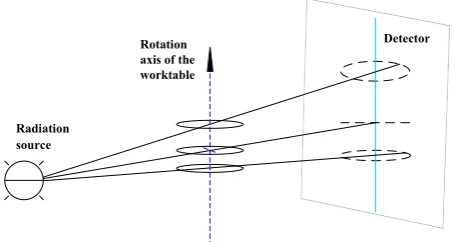
In the existing geometric calibration methods, some methods [16]-[18] use the 180° conjugate properties of the projection images to determine the rotation axis. However, during the projection process in CBCT, the ray is in the form of a cone-beam divergence rather than in a parallel form. For any point in the object to be scanned, the current projection position is not symmetrical with its corresponding projection position after 180° rotation. So this kind of methods cannot guarantee the accuracy of the calibration. It is found that the images show a symmetrical trend about the rotation axis in the images obtained by superimposing the projection images of the 360° rotary scan. As shown in Fig. 1, there are three particles with different positions. The trajectories of the three particles are circles, and the superposition image obtained by its projection images exhibits symmetrical property with respect to the rotation axis.
Detector Rotation
axis of the worktable
[image:2.595.311.542.290.391.2]Radiation source
Fig. 1. The sketch map of superimposed CBCT projection image.
Based on the symmetric principle, the rotation axis of CBCT can be calculated using the circular scan projections of the measured object itself. But the actual measured object is usually irregular, using the measured object to calibrate geometric parameters has many uncertain factors, which will bring a lot of interference to the calculation process of rotation axis. So, it is difficult to determine the exact center of the beam, and will reduce the robustness of the calibration method. At the same time, it is difficult to determine the magnification ratio of the reconstructed image by using the information of the measured object, because the measured
object itself lacks accurate and effective size values.
[image:2.595.53.282.501.622.2]Through some research and analysis, using the cylindrical object can obtain a better gray distribution in the projection image. Because fine straight wire can achieve very small geometric dimensions, good projection images can be obtained in small focus CT, particularly in micro focus CT. The contrast in the projection image is high, making it easy to analyze the gray distribution of the projection image. At the same time, the wire also has the advantages of easy access and low cost. In order to improve the robustness and accuracy of the calibration method, a plexiglass tube with wire is used as the calibration tool. The design sketch of calibration tool is shown in Fig. 2, and the enlarged part on the right side is scanning projection object. Each section of the calibration tool should ensure coaxiality. The lowermost cylinder is used to mate with the central circular hole of the rotary table. In this design, to some extent, the wire in calibration tool represents the rotation axis of the object scanning, and helps to ensure the accuracy of the measurement.
Fig. 2. The design sketch of calibration tool.
In the geometric calibration method based on wire scanning, the specific calculation steps of the beam center ( , )X Z0 0 and
rotation angle β are as follows:
1) Set the approximate distance of Dso and Dsd
according to the normal scan requirement, and use a laser level meter to ensure that the center of the radiation source is in the same plane as the center of the detector. 2) Scan the calibration tool at equal angular intervals to obtain the projection images (the number is generally much smaller than the normal scan).
3) Clip the projection images, and then obtain the logarithmic images.
4) Superimpose and average the logarithmic images to obtain the rotating superimposed image.
5) Acquire the symmetry axis of the rotating superimposed image. That is, taking a plurality of straight lines at equal interval in the rotated superimposed image, using quadratic curve to fit the gray distribution of each straight line, calculating the vertex of the fitting curve, which is the rotation center on each line.
6) Fit the obtained rotation center to obtain the linear equation of the rotation axis in the projection image. 7) The slope of the linear equation is the rotation angle β ,
and the beam center ( , )X Z0 0 is obtained by
substituting the beam center plane value into the linear equation.
B. Measurement of Distance of Dso and Dsd
the rotary table is moved in a direction that is favorable for the projection difference, and the calibration tool is projected again. The imaging relationship is shown in Fig. 3.
m
Dsd
Dso
R
2
R
1
a
2
a1a2
a
[image:3.595.52.289.90.226.2]1
Fig. 3. Imaging relationship of Dso and Dsd.
It is not difficult to obtain the following equation from the geometrical relations in Fig. 3.
1
1 2 2
2
2 2 2
tan
tan
( )
sd so
sd so
R r
a
D D r
R r
a
D D m r
= =
−
= =
− −
(1)
And then we can obtain:
2 4 2 2 2 2 2 2 2 4 2
2 1 1 2 1 2 2
2 2
2 1
2
so
R m R r R R m R R r R r
D
R R
± + − +
−
= (2)
Substituting R1 and R2 obtained from the edge detection
into (2), the larger one of the two obtain values is Dso. And then substituting Dso into (1), Dsd can be solved.
According to the above analysis, the measurement steps of obtaining the distance parameters of Dso and Dsd are as
follows:
1) Set the rotary table at normal scanning position, collect some projection images of the calibration tool, and then average them to one to reduce the noise.
2) Move the rotary table in a direction that is favorable for the projection difference, and then collect some projection images of the calibration tool and average them into one to reduce the noise.
3) Carry on the edge detection to the two projection images, respectively, and obtain the binary images including the edge contours.
4) Perform the straight line fitting to the outermost edge contours, respectively.
5) Intersect the fitted straight lines with the beam center plane, and get R1 and R2.
6) Dso is calculated according to (2).
7) Dsd is calculated according to (1).
III. EXPERIMENTS AND DISCUSSION A. Small Focus CBCT Calibration
For small focus CBCT, the measured object is usually far from the X-ray source and close to the detector, so the amplification ratio is small. The CBCT used in the experiment has been installed to ensure a certain degree of verticality and
parallelism. The diameter of plexiglass tube in the calibration tool is 30 mm, the wall thickness is 3 mm, and the wire material is copper with a diameter of 0.5 mm. Insert the calibration tool into the center hole of the rotary table. And then, approximate distance parameters can be obtained with a tape measure. Dsd is about 1220 mm, and Dso is about 950
mm. The calibration voltage is 100 kVp, and the exposure is 1 mAs.
In the experiment, the image acquisition order of the calibration tool is:
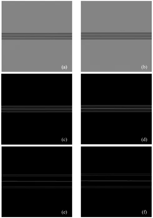
1) Collect 20 projection images at normal scanning position and average them to one (Fig. 4(a)).
2) Move the rotary table by 50 mm toward the radiation source, and then collect 20 projection images and average them to one (Fig. 4(b)).
3) Return the rotary table to normal scanning position, and circularly scan to get 72 projection images.
The above obtained projection images are cut at 2000×2000 and logarithmically calculated. Fig. 4(c) and Fig.
4(d) are the logarithmically calculated images of Fig. 4(a) and Fig. 4(b), respectively. Fig. 4(g) is the image after 72 logarithmic images were superimposed and averaged.
According to the above mentioned method, the final calculated rotation axis equation is
0.002465 1007.55
Y = − X + . So, the rotation angle β is -0.002465°. The beam center ( , )X Z0 0 is (1005.09, 1000) for
the beam center plane value Z0 is 1000. Dso is 950.50 mm,
and Dsd is 1217.85 mm.
(a) (b) (a)
(c) (d)
[image:3.595.304.549.423.772.2]Fig. 4. Projection images of calibration tool with small focus CBCT. (a) is the projection at normal scanning position, (b) is the projection at moved position, (c) is the logarithmic image of (a), (d) is the logarithmic image of (b), (e) is the enlarged edge detection image of (c), (f) is the enlarged edge detection image of (d), (g) is the image after logarithmic images were superimposed and averaged. Display window: (a) and (b) is [4000, 60000], (c) and (d) is [0, 2.2], (e) and (f) is [0, 255], and (g) is [0, 1.6].
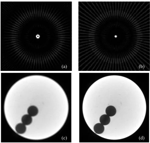
[image:4.595.302.555.205.669.2]In order to verify the accuracy of geometric parameter calibration, we compared the reconstructed images before and after calibration. Fig. 5(a) and Fig. 5(b) are the reconstructed images of the calibration tool before and after calibration, respectively. And Fig. 5(c) and Fig. 5(d) are the reconstructed images of an aluminum part before and after calibration, respectively. As can be seen, the edges of the uncalibrated reconstructed slices are blurred, and the edges of the reconstructed slices after calibration are clear and sharper. So, the image quality is significantly improved after calibration.
Fig. 5. Reconstruction results comparison of before and after calibration of small focus CBCT. (a) is uncalibrated slice image of calibration tool, (b) is calibrated slice image of calibration tool, (c) is uncalibrated slice image of test object, (d) is calibrated slice image of test object. Display window: (a) and (b) is [0, 0.5], (c) and (d) is [0, 0.04].
B. Micro Focus CBCT Calibration
For micro focus CBCT, the distance between the calibration tool and the X-ray source is very close and the amplification ratio is relatively large. In this case, the calibration tool are designed to have an outer diameter of 6 mm and a wall thickness of 1.5 mm, and the wire material is still copper and has a diameter of 0.05 mm. After the adjustment of micro focus CBCT, Dsd is about 1130 mm and
so
D is about 40 mm. The calibration voltage is 90 kVp and
the exposure is 1 mAs.
The image acquisition sequence of the calibration tool in the experiment is basically the same as that of the small focus CBCT experiment except that the move direction of the rotary table is changed to the direction toward the detector, and the move distance is still 50 mm. The images in the experiment and calculation process are shown in Fig. 6. The final calculated rotation axis equation is Y = −0.0017X+1066.05. So, the rotation angle β is -0.0017°. The beam center
0 0
( , )X Z is (1064.35, 1000). Dso is 36.45 mm, Dsd is
1129.59 mm.
Fig. 6. Projection images of calibration tool with micro focus CBCT. (a) is the projection at normal scanning position, (b) is the projection at moved position, (c) is the logarithmic image of (a), (d) is the logarithmic image of (b), (e) is the enlarged edge detection image of (c), (f) is the enlarged edge detection image of (d), (g) is the image after logarithmic images were superimposed and averaged. Display window: (a) and (b) is [0, 10000], (c) and (d) is [0, 0.8], (e) and (f) is [0, 255], and (g) is [0, 0.3].
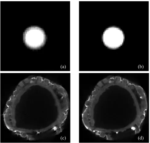
Fig. 7(a) and Fig. 7 (b) are reconstructed images of the wire before and after calibration, respectively. Fig. 7(c) and Fig. 7(d) are reconstructed images of copper gilt hairpin before
(g)
(a) (b)
(c) (d)
(a) (b)
(c)
(e)
(d)
(f)
[image:4.595.46.292.368.601.2]and after calibration, respectively. As can be seen from Fig. 7, the results of the calibration experiment are similar to those of the small focus CBCT calibration. The uncorrected edges of the reconstructed slices are blurred, and the obvious artifacts appear in the complex structures. After calibration, the corresponding artifacts are also effectively removed.
Fig. 7. Reconstruction results comparison of before and after calibration of micro focus CBCT. (a) is uncalibrated slice image of calibration tool, (b) is calibrated slice image of calibration tool, (c) is uncalibrated slice image of test object, (d) is calibrated slice image of test object. Display window: (a) and (b) is [0.3, 2.0], (c) and (d) is [0, 4.0].
IV. CONCLUSION
In this paper, based on the analysis of the existing calibration methods of CBCT geometric parameters, a fast and robust calibration method for geometric parameters based on wire scanning is proposed. The method utilizes one translation scan and one circle scan of the designed calibration tool to measure the four primary geometrical parameters directly, including the distance from the focus of X-ray source to the detector Dsd, the distance from the focus
of X-ray source to the rotation axis of the work table Dso, the
beam center ( , )X Z0 0 , and the rotation angle of the detector
β . The method has the advantages of a small amount of scanning, high measurement precision, and good robustness. The whole calibration process takes only about 3 minutes, and can be applied to different situations of the small focus CBCT and the micro focus CBCT.
REFERENCES
[1] K. D. Huang, H. Zhang, Y. K. Shi, L. Zhang, and Z. Xu, “Scatter correction method for cone-beam CT based on interlacing-slit scan,” Chinese Physics B, vol. 23, no. 9, pp. 098106, Sept. 2014.
[2] K. D. Huang, Z. Xu, D. H. Zhang, H. Zhang, and W. L. Shi, “Robust scatter correction method for cone-beam CT using an interlacing-slit plate,” Chinese Physics C, vol. 40, no. 6, pp. 068202, Jun. 2016. [3] L. A. Shepp, S. K. Hilal, and R. A. Schulz, “The tuning fork artifact in
computerized tomography,” Computer Graphics and Image Processing, vol. 10, no. 3, pp. 246–255, Jul. 1979.
[4] T. Taylor and L. R. Lupton, “Resolution, artifacts, and the design of the computed tomography,” Nuclear Instruments and Methods in Physics Research Section A: Accelerators, Spectrometers, Detectors and Associated Equipment, vol. 242, no. 3, pp. 603–609, Jan. 1986. [5] S. Tan, P. Cong, X. Liu, and Z. Wu, “An interval subdividing based
method for geometric calibration of cone-beam CT,” NDT & E International, vol. 58, no. 9, pp. 49–55, Sept. 2013.
[6] Y. Meng, H. Gong, and X, Yang, “Online geometric calibration of cone-beam computed tomography for arbitrary imaging objects,” IEEE Transactions on Medical Imaging, vol. 32, no. 2, pp. 278–288, Feb. 2013.
[7] J. Xu and B. M. W. Tsui, “A graphical method for determining the in-plane rotation angle in geometric calibration of circular cone-beam CT systems,” IEEE Transactions on Medical Imaging, vol. 31, no. 3, pp. 825–833, Mar. 2012.
[8] F. Noo, R. Clackdoyle, C. Mennessier, T. A. White, and T. J. Roney, “Analytic method based on identification of ellipse parameters for scanner calibration in cone- beam tomography,” Physics in Medicine and Biology, vol. 45, no. 11, pp. 3489–3508, Nov. 2000.
[9] B. I. Tekaya, V. Kaftandjian, F. Buyens, S. Sevestre, and S. Legoupil, “Registration-based geometric calibration of industrial x-ray tomography system,” IEEE Transactions on Nuclear Science, vol. 60, no. 5, pp. 3937–3944, Oct. 2013.
[10] J. Muders and J. Hesser, “Stable and robust geometric self-calibration for cone-beam CT using mutual information,” IEEE Transactions on Nuclear Science, vol. 61, no. 1, pp. 202–217, Feb. 2014.
[11] F. Zhang, J. Du, H. Jiang, L. Li, M. Guan, et al, “Iterative geometric calibration in circular cone-beam computed tomography,” Optik - International Journal for Light and Electron Optics, vol. 125, no. 11, pp. 2509–2514, Jun. 2014.
[12] Y. Sun, Y. Hou, F. Zhao, and J. Hu, “A calibration method for misaligned scanner geometry in cone-beam computed tomography,” NDT & E International, vol. 39, no. 6, pp. 499–513, Sept. 2006. [13] W. Dewulf, K. Kiekens, Y. Tan, F. Welkenhuyzen, and J. P. Kruth,
“Uncertainty determination and quantification for dimensional measurements with industrial computed tomography,” CIRP Annals - Manufacturing Technology, vol. 62, no. 1, pp. 535–538, Jan. 2013. [14] Y. Cho, D. J. Moseley, J. H. Siewerdsen, and D. A. Jaffray, “Accurate
technique for complete geometric calibration of cone-beam computed tomography systems,” Medical Physics, vol. 32, no. 4, pp. 968–983, Apr. 2005.
[15] J. Kumar, A. Attridge, P. K. C. Wood, and M. A. Williams, “Analysis of the effect of cone-beam geometry and test object configuration on the measurement accuracy of a computed tomography scanner used for dimensional measurement,” Measurement Science and Technology, vol. 22, no. 3, pp. 035105, Feb. 2011.
[16] M. J. Li,D. H. Zhang,K. D. Huang, S. L. Zhang, and Q. C. Yu, “Fast localization method in cone-beam computed tomography,” Acta Armamentarii, vol. 31, no. 11, pp. 1455–1460, Nov. 2010.
[17] Z. B. Wang, “Effect of center deviation on CT reconstruction images,” Acta Armamentarii, vol. 22, no. 3, pp. 323–326, Mar. 2001. [18] B. L. Li, J. Fu, Q. Z. Huang, H. Chen, and Y Wang, “One automated
method for determination of center of rotation based on sinogram in industrial computed tomography system,” Acta Aeronautica ET Astronautica Sinica, vol. 30, no. 7, pp. 1341–1345, Jul. 2009.
(a)
(c)
(b)