and winding losses must be included to provide a realistic model. In practice the losses in magnetic components give rise to signif-icant temperature increases which can lead to major changes in the component behavior. In this paper a model of magnetic compo-nents is presented which integrates a nonlinear model of hysteresis, electro-magnetic windings and thermal behavior in a single model for use in circuit simulation of power electronics systems. Mea-surements and simulations are presented which demonstrate the accuracy of the approach for the electrical, magnetic and thermal domains across a variety of operating conditions, including static thermal conditions and dynamic self heating.
Index Terms—Dynamic thermal effects, electromagnetic devices, Jiles–Atherton, modeling, simulation.
NOMENCLATURE
Thermal resistance. Power loss.
Thermal capacitance. Flux density. Field strength. Surface temperature. Ambient temperature. Flux.
Current. Voltage.
Number of primary winding turns. Number of secondary winding turns. Time.
Current monitor resistance. CH1 Oscilloscope channel 1. CH2 Oscilloscope channel 2
I. INTRODUCTION
W
ITH the advent of higher switching frequencies and power densities in power electronic circuits, it is becoming ever more important to ensure that the magnetic components in the design operate within their specified thermal, magnetic and electrical safe operating regions and performance limits. It is also becoming standard design practice to use circuit simulation software, such as SPICE or SABER, to analyze andManuscript received December 4, 2000; revised October 16, 2001. Recom-mended by Associate Editor K. Ngo.
The authors are with the Department of Electronics and Computer Sci-ence, University of Southampton, Southampton SO17 1BJ, U.K. (e-mail: [email protected]).
Publisher Item Identifier S 0885-8993(02)02176-2.
Much effort has been applied to the detailed modeling of individual components in the design, especially switching power devices such as IGBTs, power MOSFETS, and diodes [4]–[8]. Models for magnetic materials for use in power circuit simulation have included the Jiles–Atherton model [9]–[11] (implemented in many SPICE simulators and Saber), the Chan–Vladirimescu model [12] (implemented in -Spice), the Preisach model [13], [14] (implemented in Saber) and the Hodgdon model [15]–[17] (also implemented in Saber). The integration of the magnetic material models into a magnetic component model for use in a circuit simulator has been based on equivalent circuit techniques using the duality concept. Duality and the theoretical development of equivalent circuit models have been described by Cherry [18], Laithwaite [19] and Carpenter [20]. The techniques have been applied in practical examples by Zhu, Hui and Ramsden [21], [22] and Brown, Ross, Nichols, and Penny [23].
A similar approach has been used to model the relationship between power switching devices and thermal components, such as heatsinks, as shown by Hefner [4] and Hefner and Blackburn [5]. Hsu and Vu-Quoc [36], [37] have developed the use of finite element analysis to characterize detailed models for dynamic electro-thermal simulation. The effect of tempera-ture on magnetic component behavior has been examined using finite element analysis techniques, such as Jesse [24]. The development of magnetic material models that are thermally dependent has also been undertaken by Hsu and Ngo [25] and Tenant, Rousseau, and Segadi [26]., but these don’t take self heating into account. Maxim , Andreu, and Boucher [27]–[29] have implemented a lookup table hysteresis model in SPICE, with thermal behavior, but the power losses are calculated analytically and effectively restricted to fixed waveform shapes. In this paper the energy aspects of the Jiles–Atherton model of hysteresis are considered to produce the correct dynamic power loss for arbitrary applied waveforms. Winding losses and eddy current losses are also included to ensure the correct overall power loss. The resulting power loss is used as the stimulus to a lumped element thermal model including core conduction, thermal capacitance, and convection to the air. The parameters of the Jiles-Atherton model have been characterized over a wide temperature range (27 C to 154 C) and implemented in the model to vary with respect to the component temperature. This technique develops the method described by Wilson, Ross, and Brown [30].
To demonstrate the accuracy and effectiveness of the model, a standard core material was characterized (Philips 3F3) and
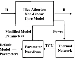
Fig. 1. Mixed domain transformer model.
Fig. 2. Pspice winding model listing.
used to create a model of a transformer for use in circuit simu-lation. Test cases were constructed and measured results com-pared with simulations.
II. PROPOSEDMAGNETICCOMPONENTMODELINCLUDING DYNAMICTHERMALBEHAVIOUR
A. Basic Magnetic Component Modeling Techniques
Modeling magnetic components for use in circuit simula-tion can take several forms. The first approach, which is gen-erally used models each magnetic component as an ideal, linear model, using inductors with coupling coefficients to represent common flux paths. This can be extended to include nonlinear couplings to represent nonlinear core materials. This method does not easily allow detailed modeling of the magnetic com-ponent behavior. Another approach is to model each winding as an interface between the electrical and magnetic domains, and define core models for the core material directly in terms of mmf and flux. This method allows the structural modeling of mag-netic components using lumped models. To illustrate this point, Fig. 1 shows a transformer modeled using two windings and a core model.
Using this mixed-domain approach is helpful in several ways. It is useful to represent the magnetic circuit with a number of el-ements representing nonlinear core sections (perhaps with dif-ferent dimensions) and linear paths for air gaps or leakage flux. An accurate model of the magnetic component can then be con-structed using these ‘building blocks.’ The inclusion of more advanced effects in the model, such as eddy currents or winding losses, can easily be included using extra elements in the model. The SPICE listings of a winding and linear core model are given in Figs. 2 and 3, respectively.
Fig. 3. Pspice linear core model listing.
Fig. 4. Modification to the Jiles–Atherton model to include temperature dependence.
B. Proposed Model Structure
It is proposed to extend the nonlinear core model by modi-fying the model parameters dynamically depending on the tem-perature of the magnetic material. The outline of the approach is given in Fig. 4. Hsu and Ngo [25] and Tenant, Rousseau, and Segadi [26] have shown how to modify the model parameters depending on the material temperature, but the temperature has been specified as a static variable. In this model, the temper-ature is calculated dynamically from a thermal network repre-senting the thermal behavior of the magnetic core. The input power to the thermal network is calculated dynamically from the nonlinear core model. It must also be noted that the power loss due to the hysteresis in the core is not the only loss to be considered, but that eddy current loss and winding losses need also be taken into account. For the moment, the eddy current and winding losses will be ignored to keep the initial model structure simple, but will be discussed later in this paper. Using this approach allows the use of arbitrary waveshapes to be ap-plied to the model and an accurate power loss estimated regard-less of the waveform. This contrasts with analytical methods of power loss calculation as described by Maxim, Andreu, and Boucher [27]–[29] for sinusoidal waveforms, which are there-fore restricted in applicability.
C. Non-Linear Core Material Model
1) Choice of Core Model: The choice of an appropriate
Fig. 5. Jiles and Atherton reversible and irreversible magnetization.
useful in frequency dependent applications. The other widely used method is the Preisach model [13], [14]. This technique has not been extensively used for circuit simulation, but mainly in finite element analysis. The main drawback of the Preisach model for implementation in a SPICE based simulator is the requirement for state based modeling which would require the development of a C or Fortran based model. In this case, the Jiles–Atherton model was considered to be useful for two specific reasons. The first reason is its implementation using simple equations with meaningful parameters. This is important when the temperature dependence of parameters is considered. If essentially arbitrary parameters as used, as in the Preisach approach, then it may be difficult to meaningfully characterize parameter variations. The second reason is the structure of the Jiles–Atherton model using separate equations for the reversible and irreversible magnetizations. Having direct access to these variable allows the power loss to be directly calculated using the model. While this does not preclude a similar approach using other models, it is a convenient aspect of the Jiles–Atherton model.
2) Implementation of Jiles–Atherton Model Using SPICE: Jiles and Atherton have developed a theory of
ferromagnetic hysteresis which separates the hysteresis func-tion into the reversible, or anhysteretic, and the irreversible, or loss, magnetizations. The magnetization is the lumped change in magnetic state when an external magnetic field is applied to the magnetic material and gives rise to an equivalent magnetic flux. Jiles and Atherton explain how the behavior of individual magnetic particles and domains can be treated as a bulk material and an effective lumped expression derived for the magnetization The total lumped magnetization as derived by Jiles and Atherton is given in (1) and illustrated in Fig. 5
(1)
The normalized anhysteretic function, , is approximated by the Langevin function as given by (2) where is the effec-tive applied magnetic field and is the parameter modifying the curvature of the function. The function must be scaled by the saturation magnetization to obtain the actual reversible magnetization
(2)
Fig. 6. Original Jiles–Atherton model implemented using Pspice.
The rate of change of the irreversible magnetization, , is ob-tained using (3), which is a lumped model of the losses caused by domain wall movement and distortion. is the total magne-tization, is the direction of the applied field strength ( for positive, for negative slope), is the permeability and is the model parameter that defines the hysteresis of the loop. The parameter a defines inter-domain coupling and is effectively a proportion of the magnetization
(3)
The total magnetization rate of change is calculated using (4), where is the parameter dictating the relative proportion of re-versible and irrere-versible magnetizations
(4)
This model has been implemented in a variety of commercial simulators, such as PSPICE and SABER, and is the de facto standard model for most nonlinear core modeling using circuit simulators. The listing of the original Jiles–Atherton model im-plemented in Pspice is given in Fig. 6.
3) Modeling Power Loss in Magnetic Components: Hefner
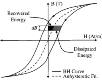
[image:3.612.65.261.63.192.2]Fig. 7. Recovered and dissipated energy in theBH loop.
The conventional method of calculating the hysteresis loss re-quires the measurement of the area of the loop. The energy lost per cycle is obtained by integrating the field strength with respect to the change in flux density . The mean power loss is found by multiplying this energy by the frequency. Un-fortunately, this procedure does not provide the instantaneous power dissipated inside the material. It is possible to make the assumption that the thermal network time constant is several or-ders of magnitude greater than that for the magnetic circuit and effectively averages out the effect of the cyclic power applied. This assumption allows the approach to be used in practical ex-amples, but the instantaneous power will still only be valid on average over the period of the simulation, not at every simula-tion point.
The Jiles–Atherton model is based on fundamental energy considerations as explained by Feynman [33] and Jiles [34] which implies that the instantaneous power loss can be derived directly from the model. The Jiles-Atherton model uses an anhysteretic function to represent the stored energy, and so the instantaneous energy loss can be approximated as shown in Fig. 7. The instantaneous power loss can be obtained by differentiating the instantaneous energy loss with respect to time. This power loss can be used as the input to a thermal circuit for a more accurate representation of instantaneous power loss. While this method is not an exact derivation of the power loss, it is an improvement over the cycle based approach and permits a more accurate estimation of the energy loss in the magnetic material for an arbitrary applied magnetic field
at all points in the simulation.
4) Modifications to the Jiles–Atherton Model to Include Dynamic Self Heating Effects: The Jiles–Atherton model was
modified as shown in Fig. 8 to use the generated temperature based on the heat flow into the thermal network to dynamically modify the model parameters. The dependence on the tem-perature was modeled using the polynomial approximations calculated from the experimental data. The heat flow into the thermal circuit was calculated using the integral of the curve to evaluate the area inside the loop.
D. Including Eddy Current Losses
The eddy current loss can be implemented in two forms. The first uses the existing Jiles-Atherton model for the core, but the model parameters are characterized with the behavior including
the eddy currents. This is apparent in a larger loop. This ap-proach is fine for a single sinusoidal frequency, but less useful in the general case for arbitrary waveforms. The second form is to dynamically include the eddy current behavior in the model. This can be achieved using inductors to model power loss in conjunction with resistors to provide the correct frequency re-sponse, or by using a filter on the applied field variable to pro-vide a larger apparent loop area at higher frequencies. In this paper, fixed frequency sinusoidal waveforms were used, and the frequencies were chosen to minimize the effect of eddy currents on the eventual thermal behavior. In this paper the a.c. resistance variations have not been included, but this could be easily implemented using an RL ladder network with the same principle.
E. Winding Losses
To include the d.c. winding losses, the winding model previ-ously given in Fig. 2 was modified as shown in Fig. 9 to extract the instantaneous power dissipation from the winding for inclu-sion as a power source in the thermal circuit.
F. Modeling the Thermal Behavior of the Magnetic Component 1) Thermal Modeling Concepts: The thermal model for
the magnetic core consists of the core thermal conduction, the thermal convection to the atmosphere and radiated emissions as described by Snelling [35]. The governing variables for the thermal system are the heat flow (or power) and the tempera-ture. In the thermal network models, the heat flow is defined as the through variable and the temperature as the across variable, analogous to the electrical current and voltage respectively. Each of the elements in the thermal network can be represented by an equivalent electrical circuit model for simulation, as described previously by Hefner and Blackburn [5] and Hsu and Vu-Quoc [36], [37].
2) Thermal Conduction Model: Snelling [35] provides the
general expression for the calculation of the conduction of heat through a lamina and hence the effective thermal resistance for a magnetic core as given in (5), where is the elemental lamina thickness, is the thermal conductivity and is the cross-sec-tional area
(5)
Practical magnetic materials are usually of a more complex shape and this requires some analysis, again described by Snelling [35], to calculate the effective thermal resistance of the material. In the magnetic core, the power source is distributed throughout the volume. To calculate the thermal resistance of a toroid, for example, requires the integration of the heat flow over the volume of the toroid. The thermal resistance relates the integration between the centre of the core and the core surface to the total power input. Equation (6) shows that the thermal resistance is dependent on the cross section diameter of the toroid
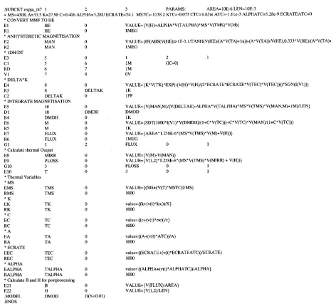
Fig. 8. Spice listing of Jiles–Atherton model extended to include parameter variations with temperature.
Fig. 9. Winding model with thermal pin connection.
The implementation of a thermal resistor in spice can be achieved using a standard resistor component, with the resistance equal to the thermal resistance.
3) Thermal Capacitance: The definition of the thermal
ca-pacitance is given by (7), where is the incremental Power Loss, is the thermal capacitance and is the rate of change of temperature
(7)
The thermal capacitance can be modeled in a circuit simulator using an electrical capacitance, where the value of capacitance is the thermal capacitance for the material. The value of thermal capacitance for a material can be calculated using the volume, density and specific heat in (8)
Volume (8)
4) Thermal Convection: The major loss of heat from the
Fig. 10. Thermal convection model.
Fig. 11. Thermal emission model.
then the convection of heat from a toroid is considered to be approximately the same as that from a cylinder, where is the temperature difference across the boundary and is the toroid diameter. In most cases a thermal resistance model is of ade-quate accuracy
(9)
The thermal convection was modeled in spice using the model given in Fig. 10.
5) Radiated Emissions: The radiation of heat from the core
is generally disregarded as it can be much smaller than the other forms of heat transfer, but can be included in a model if neces-sary for improved accuracy. The standard Stefan–Boltzman law given in (10) defines the rate of heat dissipation, where is the emissivity of the material
(10)
The thermal emission was implemented in spice using the model given in Fig. 11.
6) Thermal Network Model Implementation: In this paper,
the temperature was assumed to be constant across the volume of the core material, and therefore the thermal resistance of the core material can be ignored in this instance. If the heat transfer behavior across the core material is required, then a ladder network of thermal resistances and capacitances is nec-essary. The transfer of heat from the core to the surrounding atmosphere takes place primarily through surface convection and radiated thermal emissions. The thermal capacitance of the TN10/6/4 core is based on the volume, specific heat and den-sity of the core material. Using the Philips data book denden-sity value of 4750 kg/m , the specific heat of MnZn Ferrites given by Snelling [35] as 700–800 JKg C , and the volume of the core (188e-9 m ) the thermal capacitance was calculated to be 0.67 J C . The parameters for the convection model were based on the surface area of the toroid’s ferrite material 293 mm and diameter of 4.4 mm (see Fig. 14 for the toroid’s dimensions). The resulting thermal circuit is shown in Fig. 12. If more detail is required in the thermal model, a distributed approach can be implemented using the same basic models, as
[image:6.612.307.544.64.508.2]Fig. 12. Thermal circuit.
[image:6.612.305.555.385.545.2]Fig. 13. TN10/6/4 physical dimensions.
Fig. 14. Test configuration for temperature characterization.
described by Hefner and Blackburn [6] and Hsu and Vu-Quoc [36], [37]. The penalty for using a distributed approach would be a considerable added complexity to the circuit simulation.
III. DERIVATION OF MAGNETIC MATERIAL
MODELPARAMETERS
A. Measurement of Material Behavior
Fig. 15. BH characteristic variation with temperature.
field strength of 100 At/m. The power amplifier was con-figured as a current amplifier to ensure that the applied cur-rent and hence applied magnetic field strength was the same under all environmental and load conditions. Initially the fre-quency was set to 80Hz to minimize any eddy currents. The primary current sense and secondary voltage waveforms were captured using a digital oscilloscope and transferred to a per-sonal computer for post-processing. The flux density was derived from the (no load) secondary voltage by using numerical integration (fourth order Runga–Kutta) and the applied mag-netic field strength (H) derived from the voltage across the pri-mary current sense resistor. The environmental temperature was varied across the range 27 C to 154 C in 10 C steps by set-ting the oven temperature. The temperature was verified using a temperature probe attached to the surface of the core. The tem-perature was allowed to stabilize between measurements for a minimum of 10 min. Examples of the resulting curves ob-tained can be seen in Fig. 15. This clearly shows that as the temperature increases, the saturation flux density decreases, as does the coercive force. There is also increased loop tip closure, as has been previously investigated by Wilson and Ross [31]. Testing of the material beyond the Curie temperature (220 C) gave rise to complete thermal demagnetization as expected for this material.
B. Extraction of the Model Parameters Including Temperature Variations
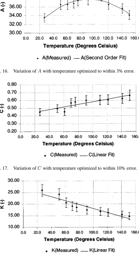
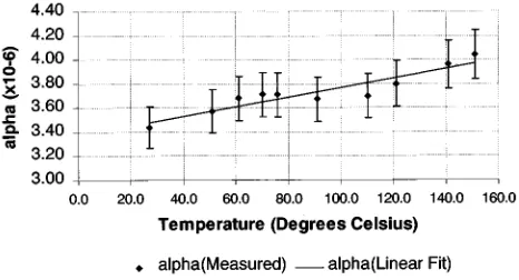
[image:7.612.309.542.65.193.2]The Jiles–Atherton model parameters were extracted from the hysteresis curves obtained at each test temperature, by optimizing the model to fit the measured data at each point. A genetic algorithm was used in this case, as has been described by Wilson, Ross, and Brown [32]. Regression analysis was ap-plied to the resulting model parameters to obtain functions for each model parameter with respect to temperature. The resulting extracted parameters, regression analysis curves and estimated errors are shown in Figs. 16–20. It is important to note that the Jiles–Atherton model parameters may be highly interdepen-dent, therefore care must be exercised in constraining the op-timization process to achieve consistency of parameter change across the temperature range. Any discontinuity in character-istic should be analyzed for “rogue” optimization results.
[image:7.612.312.540.101.523.2]Fig. 16. Variation ofA with temperature optimized to within 3% error.
Fig. 17. Variation ofC with temperature optimized to within 10% error.
Fig. 18. Variation ofK with temperature optimized to within 5% error.
Fig. 19. Variation ofM with temperature optimized to within 5% error.
C. Parameter Validation—Static Thermal Testing of Magnetic Material Model
[image:7.612.306.544.389.518.2] [image:7.612.306.546.547.674.2]Fig. 20. Variation of alpha with temperature optimized to within 5% error.
Fig. 21. Magnetic material model static temperature test circuit in PSPICE.
modification for improved early closure modeling as outlined by Wilson, Ross, and Brown [32]. The parameters were modified to include temperature dependence as characterized previously. The test circuit shown in Fig. 21 was used to test the behavior of the model. The comparison of the measured and simulated curves at 27 C, 95 C, and 154 C can be seen in Figs. 22–24, respectively. It is clear from these figures that there is an excellent correlation between the measured and simulated waveforms.
IV. EXAMPLE: MODELING ATRANSFORMERWITH DYNAMICSELF-HEATINGEFFECTS
A. Static Thermal Behavior Testing
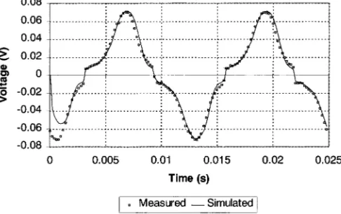
To demonstrate the electrical behavior of the model, in-cluding the effects of the thermally dependent magnetic core, an example transformer was modeled including eddy currents, winding losses and hysteresis losses, with a thermal circuit to complete the electric-thermal-magnetic model. The complete model of the transformer, thermal circuit and electrical circuit is shown in Fig. 25. A voltage was applied to the primary of the transformer at 80 Hz at 27 C and 70 C driving the transformer into saturation for a short time with the resulting simulated and measured waveforms shown in Figs. 26 and 27. The initial difference between the measured and simulated waveforms is primarily due to differing initial conditions and the waveforms correlate better after one cycle has been completed. The
simu-Fig. 22. Measured and simulatedBH curves at 27 C.
Fig. 23. Measured and simulatedBH curves at 95 C.
Fig. 24. Measured and simulatedBH curves at 154 C.
[image:8.612.42.290.235.379.2] [image:8.612.306.552.285.471.2] [image:8.612.307.550.510.694.2]Fig. 25. Electrical-thermal-magnetic transformer model in PSPICE.
Fig. 26. Measured and simulated transformer secondary voltage at 27 C.
Fig. 27. Measured and simulated transformer secondary voltage at 70 C.
and accurately predict the electrical behavior of the transformer at different temperatures.
TABLE I MEASURED AND SIMULATED
TEMPERATURERISES
B. Self-Heating and Dynamic Magnetic-Thermal Testing
With the static results showing a good correlation between measured and simulated results at a variety of environmental temperatures, the core temperature was measured and simulated due to the self heating of the core itself. For the TN10-3F3 core, a simulated temperature rise of 3.5 C corresponded well with a measured rise of 3.2 C. Measurements on a range of core types showed a thermal time constant in seconds making full real-time simulations time-consuming and memory intensive. The results of the overall temperature rise measurements and simulations are given in Table I. By reducing the thermal capacitance in the thermal model, the simulation times could be reduced but still keeping the overall temperature changes correct. An RM12 core was used to investigate the accuracy of the approach for a more complex core type.
C. Simulation of Dynamic Magnetic Material Behavior
[image:9.612.43.286.547.700.2]Fig. 28. Variation ofB with time as core temperature increases.
Fig. 29. Core surface temperature rise for insulated core.
is possible to observe the dynamic behavior of the flux in the core as the temperature increases (with the time axis effectively scaled by the reduction of the thermal capacitance). This allows reasonable simulation times to be achieved without significant loss of overall accuracy. An example of this is the variation of flux density as the core heats up (as shown in Fig. 28). In this case the simulated results of the RM12 core show a reduction in the peak flux density of 10%, which is consistent with measured values. The advantage of the simulation is the ability to observe the dynamic behavior, which is difficult to see on a real-time measurement.
The core surface temperature can also be observed in the same context as the flux density variation using this time-scaling ap-proach. Fig. 29 shows the core surface temperature rise for the RM12 core, with the time constant reduced by a factor of 10000.
V. CONCLUSION
A. Overall Conclusions
This paper demonstrates how self-heating and dynamic thermal effects can be implemented in magnetic component models for application in circuit simulators. Modeling methods have been presented to show how the Jiles–Atherton hysteresis model can be made temperature dependent and characterized. Lumped element models of thermal components were derived, and these were used to accurately model the thermal aspects of the core material and its effect on both the magnetic and electrical behavior. Good correlation between the simulated and measured results of the magnetic component in the electrical, magnetic and thermal domains has been observed, for static and dynamic temperature variations. Analysis of the methods for the calculation of power losses in magnetic materials has highlighted the need for care in the assumption of the behavior of energy losses in magnetic materials, particularly when applied to circuit simulation.
B. Validity of the Model
The model in its present form has only been tested for sinu-soidal waveforms at low frequencies ( kHz). Although the model is theoretically valid for arbitrary waveforms and higher frequencies, these have not been tested thus far, and will be the subject of future work.
C. Simulation Issues
This work has raised issues with simulating this type of mixed-domain system, the most important of these being large differences in time constants. If simulations are carried out over long periods, then it is possible for cumulative accuracy to be very poor. This paper has highlighted this and demonstrated that by judiciously reducing the thermal time constants, reasonable predictions of the overall performance can be obtained.
REFERENCES
[1] S. Chwirka, “Using simulation as an integral part of the power con-verter design process,” in Proc. IEEE Workshop Comput. Power
Elec-tron., 1994, pp. 121–126.
[2] P. R. Wilson, “Simulation of modular power systems,” in Proc. Colloq.
CAD Power Electron., 1992.
[3] , “Modeling and simulation of power factor correction circuits in-cluding automatic compliance to regulations defining current harmonic limits,” in Proc. Power Contr. Intell. Motion Conf., May 1996, p. 103. [4] A. Hefner, “A Dynamic electro-thermal model for the IGBT,” in IEEE
IAS Conf. Rec., 1992, p. 1094.
[5] A. R. Hefner and D. L. Blackburn, “Simulating the dynamic electro-thermal behavior of power electronic circuits and systems,” in Conf. Rec.
IEEE Workshop Comput. Power Electron., 1992, p. 143.
[6] , “Thermal component models for electro-thermal network simu-lation,” Proc. IEEE Semicond. Thermal Meas. Manag. SEMI-THERM
Symp., p. 88, 1993.
[7] C. L. Ma and P. O. Lauritzen et al., “A Systematic approach to modeling power semiconductor devices based on charge control principles,” in
Proc. PESC, Taipei, Taiwan, R.O.C., 1994.
[8] P. O. Lauritzen and C. L. Ma, “A simple diode model with reverse re-covery,” IEEE Trans. Power Electron., vol. 6, pp. 188–191, Apr. 1991. [9] D. C. Jiles and D. L. Atherton, “Ferromagnetic Hysteresis,” IEEE Trans.
Magnetics, vol. 19, pp. 2183–2185, Sept. 1983.
[10] , “Theory of ferromagnetic hysteresis (invited),” J. Appl. Phys., vol. 55, pp. 2115–2120, Mar. 1984.
[11] , “Theory of Ferromagnetic Hysteresis,” J. Magn. Magn. Mater., vol. 61, pp. 48–60, 1986.
[12] J. H. Chan, A. Vladirimescu, X. C. Gao, P. Libmann, and J. Valainis, “Non-linear transformer model for circuit simulation,” IEEE Trans.
Computer-Aided Design, vol. 10, pp. 476–482, Apr. 1991.
[13] F. Preisach, “Über die magnetische nachwirkung,” Zeitschrift Phys., pp. 277–302, 1935.
[14] A. Courtay, “The Preisach Model,” Analogy, Inc., Analogy Tech. Note, 1999.
[15] M. L. Hodgdon, “Mathematical theory and calculations of magnetic hys-teresis curves,” IEEE Trans. Magn., vol. 24, pp. 3120–3122, Nov. 1988. [16] , “Applications of a theory of ferromagnetic hysteresis,” IEEE
Trans. Magn., vol. 27, pp. 4404–4406, Nov. 1991.
[17] D. Diebolt, “An implementation of a rate dependent magnetics model suitable for circuit simulation,” in Proc. APEC Conf., 1992.
[18] E. C. Cherry, “The duality between inter-linked electric and magnetic circuits,” in Proc. Phys. Soc., vol. 62, 1949, pp. 101–111.
[19] E. R. Laithwaite, “Magnetic equivalent circuits for electrical machines,”
Proc. Inst. Elect. Eng., vol. 114, pp. 1805–1809, Nov. 1968.
[20] C. J. Carpenter, “Magnetic Equivalent Circuits,” Proc. Inst. Elect. Eng., vol. 115, pp. 1503–1511, Oct. 1968.
[image:10.612.64.261.205.303.2]into account the temperature,” in Proc. Eur. Power Electron. Conf., vol. 1, 1995, pp. 1.001–1.006.
[27] A. Maxim, D. Andreu, and J. Boucher, “New spice behavioral macro-modeling method of magnetic components including the self-heating process,” in PESC Rec.—IEEE Annu. Power Electron. Spec. Conf., vol. 2, 1999, pp. 735–740.
[28] , “Novel behavioral method of SPICE macromodeling of magnetic components including the temperature and frequency dependencies,”
Proc. IEEE Appl. Power Electron. Conf. Expo. (APEC’98), vol. 1, pp.
393–399, 1998.
[29] , “New analog behavioral SPICE macromodel of magnetic com-ponents,” in Proc. IEEE Int. Symp. Ind. Electron., vol. 2, 1997, pp. 183–188.
[30] P. R. Wilson, J. N. Ross, and A. D. Brown, “Dynamic electro-mag-netic-thermal modeling of magnetic components,” in Proc. IEEE Conf.
Comput. Power Electron. (COMPEL’00), 2000.
[31] P. R. Wilson and J. N. Ross, “Definition and application of magnetic material metrics in modeling and optimization,” IEEE Trans. Magn., vol. 37, pp. 3774–3780, Sept. 2001.
[32] P. R. Wilson, J. N. Ross, and A. D. Brown, “Optimizing the Jiles-Atherton model of hysteresis using a genetic algorithm,” IEEE
Trans. Magn., to be published.
[33] R. P. Feynman, R. B. Leighton, and M. Sands, Lectures in Physics, 16th ed. Reading, MA: Addison-Wesley, 1983, vol. 2, ch. 37.
[34] D. C. Jiles, Introduction to Magnetism and Magnetic Materials, 1st ed. London, U.K.: Chapman & Hall, 1991, ch. 7.
[35] E. C. Snelling, Soft Ferrites—Properties and Applications, 2nd ed. London, U.K.: Butterworth, 1988, pp. 255–264.
[36] J. T. Hsu and L. Vu-Quoc, “A rational formulation of thermal circuit models for electro-thermal simulation—Part I: Finite element method,”
IEEE Trans. Circuits Syst., vol. 43, pp. 721–732, Sept. 1996.
[37] , “A rational formulation of thermal circuit models for electro-thermal simulation—Part II: Model reduction techniques,”
IEEE Trans. Circuits Syst., vol. 43, pp. 733–744, Sept. 1996.
Swindon, U.K. During this time he developed a number of models, libraries, and modeling tools for the Saber simulator, especially in the areas of power sys-tems, magnetics, and telecommunications. His current research interests include modeling of magnetic components in electric circuits, VHDL-AMS modeling and simulation, and the development of electronic design tools.
Mr. Wilson is a member of the IEE and a Chartered Engineer.
J. Neil Ross received the B.Sc. degree in physics and the Ph.D. degree on the physics of ion laser discharges from the University of St. Andrews, U.K., in 1970 and 1974, respectively.
He is a Lecturer in the Department of Electronics and Computer Science, University of Southampton, U.K. For 12 years he worked at the Central Electricity Research Laboratories, CEGB, undertaking research on the physics of high voltage breakdown and optical fiber sensors for use in a high voltage environment. He joined the University of Southampton in 1987 and has undertaken research in a variety of fields associated with instrumentation and measurement. His current research interests include the modeling of mag-netic components for communications, instrumentation, and power applications.
Andrew D. Brown (M’90–SM’96) was born in the U.K. in 1955. He received the B.Sc. degree (with honors) in physical electronics and the Ph.D. degree in microelectronics from Southampton University, Southampton, Hants, U.K., in 1976 and 1981, respectively.
He was appointed Lecturer in electronics at Southampton University, in 1981, Senior Lecturer in 1989, Reader in 1992, and was appointed to an established chair in 1998. He was a Visiting Scientist at IBM, Hursley Park, U.K., in 1983 and a Visiting Professor at Siemens NeuPerlach, Munich, Germany, in 1989. He is currently head of the Electronic System Design Group, Electronics Department, Southampton University. The group has interests in all aspects of simulation, modeling, synthesis and testing.