The Structural Difference of Shanghai Stock Index before
and after 2008: A Copula Based Analysis
Chuan Wu1, Ke Huang2, Xue Tian2, Weikang Geng1, H. J. Cai1 1International School of Software, Wuhan University, Wuhan, China 2School of Economics and Management, Wuhan University, Wuhan, China
Email: [email protected]
Received September 5, 2012; revised October 9, 2012; accepted October 16,2012
ABSTRACT
The year 2008 witnessed the greatest joint stock reform and financial crisis in Chinese history. After these two cases, significant changes have taken place in investors’ behaviors worldwide, along with which is the occurrence of structure change in stock market. In this paper, we employ Copula model to simulate the joint distribution between Shanghai Stock Index (SSE) and Chinese Shanghai Index 300 (CSI 300), to find out structure change in Chinese stock market before and after 2008. From results of empirical studies, we get conclusions that the main nature of Chinese stocks market is symmetric, in both marginal and joint distributions. Via the changes of Copula types, upper and lower tail coefficients and Kendall coefficients, we can measure the structure change in Chinese stock market, and get further con-clusion about investors’ behaviors change. Before 2008, there is an equal power in quitting market and longing, while diversified investors adjusted their expectation uniformly after this year. Testing results show that the general depend-ence structure of CSI 300 and SSE is highly dependent and symmetric in most cases. From the distribution of upper and lower tail coefficients, we can draw the conclusion that stratified investors are mainly focused on two tasks, after this year, to close the position on stocks with high correlated stocks market and to maintain market value of stocks.
Keywords: Copula Distribution; EM Algorithm; Kendall Tau Upper; Lower Tail
1. Introduction
The year 2008 has imposed remarkable influence on stock market worldwide, because of two significant cases, the joint stock reform and financial crisis. The 2008 fi-nancial crisis created strong and deep psychological fluence on investors, while serious problems were in-duced by the incomplete joint stock reform and unrea-sonable reallocation of shares between stock holders. CSI300 is a major reflection of overall price trend of Chinese stock market. It experienced a sharp decrease in 2008, from 5062.26 to 1606.73 in just 10 months. Simi-larly, another comprehensive index, SSE, also declined severely, from 4695.80 to 1664.93. Such remarkable change in Chinese stock market undoubtedly generated investors’ distinct behaviors before and after 2008. Since the main nature of Chinese stocks market is the symmet-ric marginal and joint distributions, and great changes of investors’ behaviors would contribute to the changes of marginal and joint distribution of stocks. In this paper, we will introduce Copula model to analyze the structure difference of Shanghai Stock Index before and after 2008.
Since CAPM and Black-Scholes models were pro-posed to simulate the joint distribution, many following researchers have found an obvious deviation of empirical
evidence from the theoretical model [1]. Many papers tend to ascribe it to the assumption of normality [2]. Based on overwhelming empirical evidence and discus-sions, various alternative models with non-normality are proposed, one of which is the Copula model proposed by Sklar in 1959 [3]. It is an exact and overall statistical method to describe the dependent structure between ran-dom variables by linking the marginal distribution of each [4,5]. The introduction of Copula model can im-prove the properties of estimation to fit the volatility, provide flexibility to depict the fat tail, high skewness as well as other non-normality in distribution, and solve the dimension disaster when estimating multivariate joint distributions. Its special fitness in dealing with monotone mapping variables, describing linear or non-linear de-pendence structure, symmetric or asymmetric between upper and lower tail and showing time series characteris-tics of data dynamically, makes it a promising method and gaining more and more popularity in financial re-searches such as price derivatives, financial calculations, risk management and financial fluctuations description [6-8].
Copula, and Gaussian mixture Copula is estimated as dy-namic mixture Copula to improve the fitting. With fluc-tuations and changes in stock market, any solo Copula model fails to simulate the joint distribution of two stocks without loss of accuracy in long term. A structure change in stock market can be reflected in the changes of Copular types. In this paper, we will develop the Copular model to describe the structure changes before and after 2008 due to the influences of joint stock reform and financial crisis. Based on results of empirical study, we get further conclusion about changes of investors’ be- haviors.
2. Copula Model Selection
Various Copula models are chosen to simulate the joint distribution of two stocks. They go into two major kinds: Elliptical and Archimedean Copulas.
2.1. Elliptical Copulas
2.1.1. Bivariate Gaussian Copula
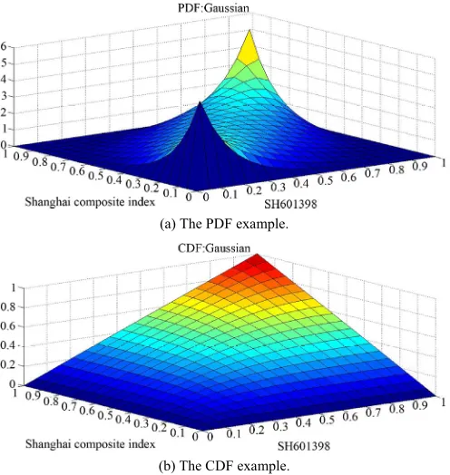
Bivariate Gaussian Copula is a symmetry distribution with asymptotically independent in both upper and lower tail. Because of the relatively easy estimation of parame-ters in this model, it fits well when the market does not fluctuate much. However, it ignores extreme incidence in the financial market.
Let be the inverse function of standard nor-mal accumulative probability function and
model can be expressed as below. The Probability Dis-tribution Function (PDF) and the Cumulative Distribu-tion FuncDistribu-tion (CDF) of Bivariate Gaussian Copula for Shanghai Stock Index are as shown in Figure 1.
u1
1, 1
be the correlation coefficient. Bivariate Gaussian Copula
2 21 1
2
2 2 1
2 1
, , e d d
1
r s rs
u v
g
C u v r s
, ,
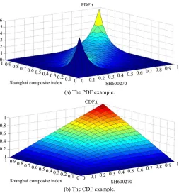
2.1.2. Gaussian Mixture Copula
Gaussian mixture Copula is a linear combination of Gaus-sian Copulas and also one of the applications of Hidden Markov Model (HMM). The HMM model describes a stochastic process with several possible states. The ran-dom variable jumps between these states ranran-domly. The HMM with Gaussian mixture is divided into two parts: a Markov chain and a stochastic process. The Markov chain measures the state switching process between different states while a stochastic process describes a dynamic process in a certain state. Since no one can specify which state the variable is experiencing, the model is called Hidden Markov Chain.
Let μ, σ denote the volatility and mean of variables, which can vary in different states. Then 11 12 13 means that there are three major states in the market for variable μ1, namely: good, medium and low condition. The random variable jumps between states with probabil-
1, 2, ,n
1 1 n
i i
and
. Gaussian mix- ity ture Copula model can be expressed as below.
(a) The PDF example.
[image:2.595.174.422.459.721.2](b) The CDF example.
2 2
1 1 2 2
2 2
1 2
2 2
k k
k k
x x
1 1 1 1
2 1 2
1
2 2 1
1 2 2
=1 1 2
1
, e
2π 1
k k k
k k k
x x
n
k
k k k k
f x x
2.1.3. Bivariate t-Copula
Bivariate t-Copula is a symmetric distribution with two equal tails, and is one of the substitute models for Gaus-sian distribution. With 1 .
representing the inverse of t distribution with degree of freedom υ. t-Copula have two parameters υ, ρ determining the structural depend-ence. These two parameters can control the peaks and tails, thus enabling more freedom in depicting the non- normality in return distributions. Expression of this Cop-ula model can be described as below. The PDF and CDF of Bivariate t-Copula for Shanghai Stock Index are shown in Figure 2.
1 1
2 2
2
2
, , , 1
1
u v
t
r s C u v
2 2
d d
rs
r s
2.2. Archimedean Copulas
2.2.1. Gumbel Copula
Gumbel Copula is asymmetric with a probability density function fatter in the upper tail and thinner in the lower tail like a “J”, which makes it very sensitive in the upper tail. In other words, there exists a better ability for it to describe the bull market. Let
then the two assets are highly correlated in the upper tail and vice versa. The PDF and CDF of Gumbel Copula for Shanghai Stock Index are shown in Figure 3.
0,1
0
be a coefficient of dependence, it can be expressed as below. If
,
1 1
log log
, , , e u v
G
C u v
Gumbel Copula fits to simulate the dependence of two assets that are highly correlated in a bull market. How-ever, since it is insensitive to changes in the lower tail, Gumbel Copula is not suitable in a bear market, less able to model lower tail, which is independent.
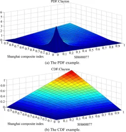
2.2.2. Clayton Copula
Let 0, be the coefficient to depict dependence. If
, it indicates the two assets are highly depend-ent in lower tails which is just the reversed case of Gumbel Copula like and “L”. The PDF and CDF of Clayton Copula for Shanghai Stock Index are shown in Figure 4.
1
, , 1
C
C u v uv
In contrast with Gumbel Copula, it is more sensitive to bear market, and specially fits to simulate the depend-ence structure of two assets in bear market.
(a) The PDF example.
[image:3.595.149.444.87.129.2](b) The CDF example.
[image:3.595.171.424.449.721.2](a) The PDF example.
[image:4.595.171.425.82.354.2](b) The CDF example.
Figure 3. The PDF and CDF example of Gumbel Copula.
(a) The PDF example.
(b) The CDF example.
Figure 4. The PDF and CDF example of Clayton Copula.
,
, 0. When 0
2.2.3. Frank Copula
where
1 e 1
, , log 1
F
C u v
1 e
1 e
u v
u
0, the two assets are asymptotically independent. If
0 , they are
positively correlated while if , they are negatively correlated.
[image:4.595.171.426.382.649.2]upper tail and the lower tail. However, it cannot capture asymmetric dependence. Unlike t-Copula, it has both fat tails and higher correlation in the middle of the distribu-tion while t is thinner.
2 =1 , , nIP iI ip
iI iP i
C u F v F
L u v f f
u v
3. The Measure of Dependence Structure
3.1. Kendall Rank Coefficient τ
To analyze the correlation between variables, we intro-duce Kendall rank correlation coefficient (τ) which is represented by corresponding Copula function as
v C u vd , 1
1 1
0 0
4 C u,
3.2. Upper and Lower Dependence
Upper and lower dependence statistics are introduced to measure the association between two quantities. Define the joint survival function of Copula as C · ·,
1u,1v
,where
ˆ , 1
C u v u v C
Let X,Y be two continuous random variables with mar-ginal distribution F
· and G
·
· ·,
. Specify the Copula asC , then the Upper tail dependence up
and lower dependence low are defined as follows:
up 1 1
1 1 1 1
lim lim lim lim
u u P Y G u X F u u u
ˆ 1 ,1 1
C u u u
low 1 1
0 0 0 0
lim lim lim lim
u u P Y G u X F u u u
ˆ 1 ,1 1
C u u
u up
If or low exists and up or low
0,1
, they measure the dependence structure in extreme cases;ifup
or , then, they are statistically independ-ent. It is very easy to observe whether the collapse of one asset’s price will be followed or lead to the others’ col-lapse with these measure dependences.
low
0
4. The Estimation of Copula
4.1. Estimation of Static Copula
As assumed in Sklar’s theorem, if the marginal distribu-tions of variables are all continuous, then there must ex-ists one Copula that fits their joint distribution. Suppose F
u v, is the joint distribution with marginal distribu-tion 1
, . A unique Copula C u existssatisfying: .
F · F2
·
,v
u v,
,F C u v
The estimation of Copula and the marginal distribution can be very time consuming and cumbersome with ordi-nary MLE method. We employ a two stage MLE method to improve the accuracy and optimize the algorithm of static Copula, include Gauss Copula, t-Copula, Frank Cop- ula, Clayton Copula and Gumbel Copula. Suppose there are n samples and the likelihood function is:
2 , ,
I
where i CP u v u F viI Fip
u v
=1 =1 =1
ln , , ln ln
n n n
i ip iI
i i i
L
c u v
f
f1 ln n ip i c
and ln
f
1 ln n iI iand f
The first stage is to estimate
,
f f
1
ln , , n
i i
c u v
respectively with ordinary MLE methods. The second step is to transform the estimated iI iP into cumula-tive probability value in each sample and substitute them
. Then the only unknown vector is θ, intowhich can be estimated by ordinary MLE.
4.2. Estimation of Gaussian Mixture
The estimation method for Gaussian mixtureis different from that of static Copula. Here the Expectation-Maxi- mization (EM) algorithm is employed to estimate the parameters of Gauss mixture. It is a MLE method where the model depends on unobserved latent variables. In addition, it is also an iterative method and therefore a computer program can be designed to solve them effi-ciently. In this case, the data is just like the shadow pro-jected by many normal regimes and the target is to find how many regimes and what each regimes looks like exactly [9].
1
=1 1 =1 , , n
i i t
i
k n
i t i
x p k x p k x
where
2 1 =1 2 1 =1 , , n ti k i
i
k n t
i i
x p k x p k x
2 1 =1 2 1 =1 , , n ti k i
i
k n t
i i
x p k x p k x
where
2 1 =1 2 1 =1 , , n ti k i
i
k n t
i i
x p k x p k x
2 1 =1 2 1 =1 , , n ti k i
i
k n t
i i
x p k x p k x
The upper limit of regimes of Gaussian mixture is 10. For the determination of regimes of Gaussian mixture, the following procedures are suggested [10]:
2 2
1 1
ˆt ˆt
u
2) Estimated the parameters with assumption of M re-gimes.
does not mean there is no approximate one to estimate. We use Kernel smoothing density estimation as an as-ymptotic distribution of those ones [15]. In essence, it is a weighted average between sample points by using ker-nel function as weighted functions. Generally, we em-ploy the standard normal distribution as the kernel func-tion for it is widely used in distribufunc-tion [16]. It can also be shown that the estimated parameter is asymptotically unbiased estimator of the real distribution as n approaches positive infinity [17].
3) Test the model with Kolmogorov-Smirnov (K-S) test under confidence level of 95%.
4) If the test is past, then the result is what we need. If not, let M = M + 1 and return to Step 1.
Results of univariate Gaussian mixture distribution will be candidates of marginal distribution, while that of Bivariate Gaussian mixture is used to simulate the joint distribution in our empirical study. In this paper, we use AIC, BIC and Chi square test to choose a more
appropri-ate one among these models [11,12].
5. Modeling the Return
5.1. Sample Description 4.3. The Estimation of t Copula
For the fitting extent of t Copula, there is a mature and precise way to estimate the parameters so that the time series effect can be taken into consideration. Patton firstly set up a research about how a Copula evolution equation, like ARMA (1,10) model, describes the actual trend of certain price process, leading to the study of time-varying Copula. Kole, Koedijk and Verbeek proposed some ways of choosing Copula functions. Following these studies, a Copula-GARCH model can be obtained as follows.
Previous research strongly suggest that GARCH (1,1)-t
can reflect the lag in time series [13]. We continue to employ the same model in this paper. Let ri be the returns of a stock, then GARCH (1,1)-t model can be solved as below:
2
ˆ
t t
r C u ˆ2
t K
If F · ·, ,,·
is a N-dimension joint distribution func-tion with marginal distribufunc-tionF1
· ,F2 · , , FN
· . There exits a Copula function C
··, , ,·
such that
1, 2, , N
1
1 , 2 2
F X X X C F X F X , , FN XN
While studying time-varying situation, we usually con-sider correlation parameters of Copula evolution equa-tion [14]:
1 1
t i t i
u v
log log ,
r P P
1
1
1
ˆ q
t t
i
q
In this paper, we choose Shanghai Stock Index and CSI 300 as a sample. Data from period 2005.6-2007.12 are treated as sub-sample before 2008 while 2008.1-2010.6 as the one after 2008. To calculate a specific return rate, we use i i t, i t, 1 where i is the trading code during CSI 300 and t is the specific trading day. Descrip-tion of return rate data is shown in Table 1.
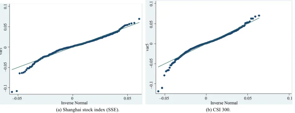
We employ two approaches to test whether the returns are normal, Q-Q plot and K-S test. If their distribution is normal, they should be consistent with the line y = x in the Q-Q plot. Moreover, in the Kolmogorov-Smirnov test, if the null hypothesis is true, namely the returns are nor-mal, the test value should be greater than 0.01. Accord-ing to the results in Figure 5 and Table 2, both Q-Q plot and K-S test show a deviation from normality of return rate of SSE and CSI 300. In other words, these results contradict the traditional assumption of Brownian mo-tion.
5.2. Modeling the Marginal Distribution
From the above discussion, non-normal models are ap-propriate to simulate marginal distributions. In this paper, we mainly use t distribution and univariate Gaussian mixture distribution model. The former one can better model the fat tails if they are symmetric while the latter is more suitable to model the asymmetric tails. In t dis-tribution model, the fatness of the tails is variable and controlled by the value of parameter nu. A small nu gives heavy tails. While for Gaussian mixture, it mainly de-pends on the different regimes to model the asymmetric tails. Theoretically, the more regimes employed in the model, the more precisely the simulation will be (of course it is possible to over specifying, so that AIC and 4.4. Kernel Smoothing Density Estimation
[image:6.595.60.545.689.737.2]However, there is a possibility that both t and Gaussian mixture are not capable of passing the test, to simulate marginal distribution of stocks exactly. In this case, we will specify them as inability to find real model. But it
Table 1. The summary statistics of return rate.
Mean Variance Skewness Kurtosis Max Min
SSE 0.0025437 0.0003866 –0.8096452 6.970561 0.0690344 –0.1107323
(a) Shanghai stock index (SSE). (b) CSI 300.
[image:7.595.68.275.311.366.2]Figure 5. The Q-Q plot of the return rate series.
Table 2. Kolmogorov-Smirnov test for normality. Skewness/Kurtosis Tests for Normality
Variable Pr (Skewness) Pr (Kurtosis) adj chi2 (2)
SSE 0.000 0.000 0.000
CSI 300 0.000 0.000 0.000
BIC will set up punitive function to deal with over spe-cifying problem). For t distribution, ordinary MLE me-thod is enough to estimate parameters while a simpler EM algorithm estimates the parameters of the subsequent one.
We apply these distribution models to simulate the marginal distribution of constituent stocks of CSI300 before and after 2008, and results of their types are shown in Table 3. From the “invalid” figures, it can be easily inferred that the ability of t and Gaussian mixture to model the return after 2008 is better than that before 2008. Actually, neither of t distribution nor Gaussian Mixture distribution model fits to simulate the marginal distribution of these 300 constituent stocks before this year, thus we use Kernel smoothing density estimation for simulation. After 2008, we see that the numbers of both t and Gaussian mixture distributions increase greatly and they simulate their distributions well.
[image:7.595.335.512.322.371.2]The changes of marginal distribution reflect the struc-ture change in the stock market, which can be explained by the hedging strategy and other behaviors of investors in this particular year. Before 2008, we were not able to simulate returns of a large proportion of stocks owing to the lack of uniform behavior from traders and other in-vestors. Owing to different expectation towards stocks, there might be different peaks in the distribution, while a slight decline will cause different reactions: some quit but some continue to hold long stocks. When the domi-nating power switches, the divergence from normality was hard to capture. However, after 2008, the behaviors
Table 3. Types of marginal distribution of constituent stocks of CSI300 before and after 2008.
Marginal Distribution
t Gaussian Mixture Invalid
Before 41 158 101
After 84 207 9
of investors are much more uniform. The increased num-ber of t distributions illustrates the symmetric character-istics in both upper and lower tails, reflecting the equal power in quitting market and longing. Fewer investors stay put during 2008. For Gaussian mixtures, a sudden increase might suggest that stratified investors start to dominate the market after 2008. Although they have dif-ferent preference for risk, after the crisis, diversified in-vestors adjusted their expectation uniformly so that the regimes switching model are specified. We simulate the marginal distribution of CSI300 constituent stocks, and find that large part of them change marginal distribution types after 2008. Detailed information of a small sample is shown in Table 4.
5.3. Modeling the Joint Distribution of Copula
After fitting the marginal distribution, then the joint dis-tribution can be found by the two stage MLE method. The general results are shown in the Table 5.
From Table 5, one interesting fact is that both Clayton and Gumbel Copula that are good at modeling bull and bear market are not specified here. On the contrary, the results of model fitting mainly show the symmetric de-pendence structure both before and after 2008. Before 2008, the t-Copula is most frequent, while after 2008, t
the general dependence structure of CSI300 and SSE is symmetric in most cases.
5.4. Measure of Correlation in Overall Level
[image:8.595.59.287.261.349.2]Besides, the positive correlation can also be found in the Kendall tau rank correlation. The distribution of Kendall tau rank correlation of CSI300 and SSE is shown in Fig-ure 6. In fact, the rank correlation coefficients show a highly explicit dependence structure of CSI 300 and SSE, which gives the reason why symmetric Copula is pre-vailing.
Table 4. Marginal distributions of constituent stocks of CSI300 before and after 2008.
Code Before After Code Before After SH600016 - t SZ000002 GausMix t SH601328 GausMix t SZ000858 GausMix t SH600000 GausMix t SH600837 GausMix t SH601166 GausMix t SH601398 GausMix t SH600519 t GausMix SH601601 - GausMix SH601088 - GausMix SH601668 - t
Table 5. Frank and Gumbel Copula dominate after 2008 and not t and Frank.
Copula types
Gaussian t Clayton Frank Gumbel before 4 162 46 15 2
[image:8.595.57.286.385.527.2]after 8 150 14 116 4
Figure 6. The Kendall tau of CSI300 and SSE.
5.5. Measure of the Dependence in Extreme Cases
The dependence structure in extreme cases is a very im-portant issue in empirical studies. For example, the joint stock reform and financial crisis are extreme cases, and here we employ upper and lower tails coefficient to fig-ure out the changes in structfig-ure of Chinese stock market. Statistics about a small sample from CSI300 constituent stocks are shown in Table 6.
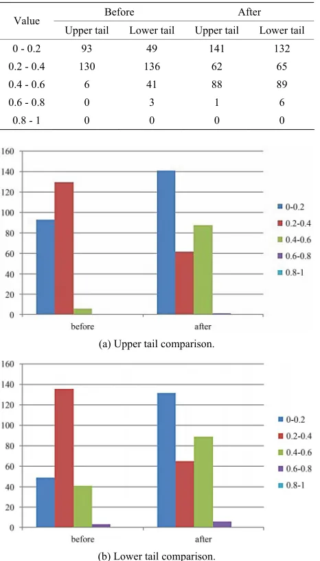
Collect test results of CSI 300 constituent stocks with SSE, we get the statistical results in Table 7. It shows that the value of upper and lower tails coefficients in-crease after 2008, which implies a stronger tendency that CSI300 and SSE are more correlated with each other in extreme cases. In both cases, upper tails and lower tails are scattered similarly, echoing to the prior finding of the symmetric Copula. The distribution of upper tail and lower tail are very similar, as shown in Figure 7. Before 2008, they are most aggregated in 0.2 - 0.4, while after 2008; there are two intervals that are aggregated 0 - 0.2 and 0.4 - 0.6.
From other points of view, if the same categories of coefficient were put together, it might bring our attention that another structural change is the extreme cases for some stocks, like those stocks with lower tail lying in 0.6 - 0.8. The main nature of CSI 300 after 2008 can be di-vided into two types: the first one is that a majority of constituent stocks in CSI300 continue to perform against the trend of SSE, or simply suffer from a small slump. For some additional stocks, the second large proportions of them are highly correlated with SSE, which in turn suffer a great loss, just like SSE.
[image:8.595.69.527.562.734.2]Therefore, one important fact deduced from it is that the formerly mentioned stratified investors are mainly focused on two tasks. The first one is to close the posi-tion on these stocks with high correlated stocks market.
Table 6. Acomparison of sample stocks’ test results before and after 2008.
Copula type Upper tail Lower tail Kendall rank Code
before after before after before after before after
SH600036 Gumbel t 0.5377 0.4793 0.1171 0.4793 0.6222 0.8061
SH600016 Frank t 0.0562 0.5342 0.0562 0.5342 0.7068 0.8307
SH601318 Clayton t 0.0201 0.5060 0.5120 0.5060 0.4868 0.8118
SH600000 Frank t 0.0562 0.4661 0.0562 0.4661 0.7070 0.7971
SH601088 - t - 0.5501 - 0.5501 - 0.8064
SH601398 Gaussian t 0.3652 0.5000 0.3652 0.5000 0.7765 0.7920 SH601601 - Frank - 0.0869 - 0.0869 - 0.8488
SH601668 - t - 0.3418 - 0.3418 - 0.6935
SH601939 - t - 0.5519 - 0.5519 - 0.8098
SH601169 - t - 0.5126 - 0.5126 - 0.8112
Table 7. A comparison of upper and lower tails coefficient before and after 2008.
Before After Value
Upper tail Lower tail Upper tail Lower tail
0 - 0.2 93 49 141 132
0.2 - 0.4 130 136 62 65
0.4 - 0.6 6 41 88 89
0.6 - 0.8 0 3 1 6
0.8 - 1 0 0 0 0
(a) Upper tail comparison.
(b) Lower tail comparison.
Figure 7. The comparison of upper and lower tail coeffi-cient before and after 2008.
These strategies intensified the collapse of the market. The second one is to maintain market value of stocks so that these stocks perform a less correlated dependence structure.
5. Conclusion
This paper mainly discusses the structural changes before and after 2008 with the application of bivariate Copula to measure the joint dependence between CSI300 and SSE. Firstly, the non-normality characteristic is found in the marginal distribution. Before 2008, investors’ behaviors are so various that marginal distribution models fail to simulate them well, but after it, the marginal distribution is better specified by t and Gaussian mixture distributions.
Although there is a collapse of market, the return distri-bution remains relatively symmetric by comparison of types of Copula. It might be explained by the stratified investors’ distribution. There is a group of investors who want to quit the market or close the position while an-other requires hedging strategies to maintain the value. In addition, we examine the value of Kendall tau, upper and lower tail to support the investor’s constitution. The Kendall tau shows a medium correlation of CSI 300 and SSE. After 2008, the upper and lower tail also shows a two-peak in its value interval distributions. Thus, it can be concluded that the structural change, with a sudden change of the tendency of SSE, leads to a multidimen-sional influence on the behavior of CSI 300 and investors. The peer effect might gather uniformly distributed types of investors into several main groups that remain univer-sal nature in a certain group. With this change in inves-tors’ expectations and strategies, the marginal distribu-tion of return deviates from normal distribudistribu-tion symmet-rically and asymmetsymmet-rically. And the joint distribution is more symmetric with medium correlation of market be-cause two powers are offset to a certain extent.
REFERENCES
[1] C. Jacky, “Some Empirical Evidence on the Outliers and the Non-Normal Distribution of Financial Ratios,” Jour-nal of Business Finance & Accounting, Vol. 14, No. 4, 1987, pp. 483-496.
doi:10.1111/j.1468-5957.1987.tb00108.x
[2] X. Z. Bai, “Beyond Merton’s Utopia: Effects of Non- Normality and Dependence on the Precision of Variance Estimates Using High-Frequency Financial Data,” The University of Chicago, Chicago, 1999.
[3] A. Sklar, “Fonctions de Repartition à n Dimensions et Leurs Marges,” Publication de l’Institut de Statistique de l’Université de Paris, Paris, 1959, pp. 229-231.
[4] R. B. Nelsen, “An Introduction to Copulas,” 2nd Edition, Springer, Berlin, 2006.
[5] E. Jondeau and M. Rockinger, “The Copula-GARCH Model of Conditional Dependencies: An International Stock-Market Application,” Journal of International Money and Finance, Vol. 25, No. 5, 2006, pp. 827-853. doi:10.1016/j.jimonfin.2006.04.007
[6] H. Joe, “Multivariate, Models and Dependence Con-cepts,” Chapman & Hall, London, 1997.
[7] A. J. Patton, “Estimation of Multivariate Models for Time Series of Possibly Different Lengths,” Journal of Applied Econometrics, Vol. 21, No. 2, 2000, pp. 147-173. doi:10.1002/jae.865
[8] A. J. Patton, “On the Out-of-Sample Importance of Skew-ness and Asymmetric Dependence for Asset Allocation,” Journal of Financial Econometrics, Vol. 2, No. 1, 2004, pp. 130-168. doi:10.1093/jjfinec/nbh006
Statistical Society, Series B, Vol. 39, No. 1, 1977, pp. 1-38. [10] C. Genest, J.-F. Quessy and B. Rémillard, “Goodness-
of-Fit Procedures for Copula Models Based on the Prob-ability Integral Transformation,” Scandinavian Journal of Statistics, Vol. 33, No. 2, pp. 337-366.
doi:10.1111/j.1467-9469.2006.00470.x
[11] F. X. Diehoid, et al., “Evaluating Density Forecasts with Application Financial Risk Management,” International Economic Review, Vol. 39, No. 4, 1998, pp. 863-883. doi:10.2307/2527342
[12] I. Karatzas and S. Shreve, “Methods of Mathematical Finance,” Springer-Verlag, Berlin, 1998.
[13] H. J. Cai, H. Sun, C. Wang and Y. Wang, “A Cop-ula-GARCH Analysis of Chinese Stock Market Depend-ence Structure,” Advances in Intelligent and Soft
Com-puting, Vol. 136, 2012, pp. 589-596.
[14] C. Jacky, “Some Empirical Evidence on the Outliers and the Non-Normal Distribution of Financial Ratios,” Jour-nal of Business Finance & Accounting, Vol. 14, No. 4, 1987, pp. 483-496.
doi:10.1111/j.1468-5957.1987.tb00108.x
[15] J. Durbin, “Weak Convergence of the Sample Distribu-tion FuncDistribu-tion When Parameters Are Estimated,” The An-nals of Statistics, Vol. 1, No. 2, 1973, pp. 279-290. doi:10.1214/aos/1176342365
[16] B. L. S. PrakasaRao, “Nonparametric Functional Estima-tion,” Academic Press, Orlando, 1983.