Master Thesis - Confidential Draft
Investigation on factors limiting the
performance of deep sleep classification
Author:
Yuan Lu
Supervisor:
Mannes Poel
Pedro Miguel Fonseca
Gary Garcia Molina
Femke Nijboer
Human-Media Interaction Program
Faculty of Electrical Engineering, Mathematics and Computer Science
The content of this document is intended for reviewing by the supervisors stated above.
Contents i
1 Introduction 1
1.1 Objectives . . . 2
1.2 Methods . . . 2
1.3 Organization . . . 3
2 Background 4 2.1 Sleep physiology . . . 4
2.2 Unobtrusive sleep staging . . . 7
2.3 Framework for deep sleep classification . . . 8
2.3.1 Feature overview . . . 9
2.3.2 Cardiorespiratory features . . . 10
2.3.3 Feature normalization . . . 12
2.3.4 Classification . . . 14
2.4 Initial results . . . 14
3 Methods 21 3.1 Experimental setup and Dataset . . . 21
3.2 Hypothesis 1 validation: Regression analysis . . . 22
3.2.1 Equation and parameter estimation . . . 23
3.2.2 Evaluation of a linear regression model. . . 25
3.3 Hypothesis 2 validation . . . 26
3.3.1 Classification . . . 26
3.3.2 Experiment procedure . . . 29
3.3.3 Evaluation of hypothesis 2. . . 30
3.3.3.1 Feature evaluation . . . 31
3.3.3.2 Classification evaluation. . . 32
4 Results and Discussion 36 4.1 Validating hypothesis 1 . . . 36
4.1.1 Variables . . . 36
4.1.2 Regression analysis with one independent variable . . . 41
4.1.3 Regression analysis with more independent variables . . . 47
4.2 Validating hypothesis 2 . . . 53
4.2.1 Upper bound . . . 53
4.2.2 Subject-dependent model based on whole-night data . . . 54
4.2.3 Subject-dependent model based on cycles . . . 56
5 Conclusions 61
6 Future work 63
Introduction
Sleep is important for people. People spend nearly half of their lifetime in sleep. Sleep
problems are harmful for health. Lots of people suffer from sleep problems, such as sleep
apnea, insomnia and sleep deprivation etc. These sleep problems interfere with normal
physical and mental functioning of human body. About 17-24% of North American
adults are affected by obstructive sleep apnea, which increases the risk of sudden death
[1]. A lot of people, who do not have sleep disorders, still struggle with tiredness and lack of motivation resulted from sleep. Therefore, sleep studies emphasizes on
identify-ing elements interferidentify-ing with sleep in order to design interventions aimidentify-ing at relievidentify-ing
symptoms of sleep disorders and improving sleep quality.
Conventional sleep monitoring procedure and interpretation of sleep recordings are
cum-bersome tasks. Automatic sleep staging system is therefore developed to remove human
factors in the interpretation of sleep recordings. Other modalities for sleep monitoring
are investigated as well, such as cardiorespiratory signals which exhibit sufficient ability
in sleep staging. The new monitoring modality shows the possibility for the development
of unobtrusive sleep monitoring.
Among different sleep stages, deep sleep is an important sleep stage. The importance of
deep sleep in learning have been proved [2][3]. The features differentiating sleep stages and various classifiers are largely investigated for the sleep classification. Yet studies on
the elements limiting the performance of sleep classification has received little attention
so far.
1.1
Objectives
An early investigation of the deep sleep classification was conducted prior to this
re-search. The early investigation aimed at utilizing features, which were derived from
cardiorespiratory signals, on the deep sleep classification. The result of the early
inves-tigation indicates some aspects which may limit the performance of deep sleep
classifi-cation.
Two aspects are explicitly stated that influence the classification performance. Although
a series of features, which are dedicated to the discrimination between deep sleep and
non-deep sleep, are extracted from the cardiorespiratory signals, there are still
char-acteristics of deep sleep that are not captured by these features. For example, the
discontinuity of deep sleep, which illustrates a considerable correlation with the
classi-fication performance (Spearman ρ = −0.5), is not reflected in the extracted features.
Therefore, we suspect the classification performance depends on not only the
quali-ty of the extracted features, but also some characteristics of deep sleep external to the
extracted features. Another aspect limiting the classification performance is the
subject-independent property of the constructed classification model. This property ensures that
the model performs good in general, but is not able to consider the characteristics in
the features for specific subjects. Thus, we suspect the classification performance can
be improved if a personalized classifier is constructed.
Based on the two aspects introduced above, two hypotheses are formulated accordingly.
The first hypothesis deals with the relationships between classification performance and
deep sleep characteristics. The second hypothesis concerns the improvement brought by
personalized classifier. The scope of this master project is focused on the validation of
the two hypotheses. The validation of the two hypotheses can provide guidance for the
future work of deep sleep classification.
1.2
Methods
The validation of the two hypotheses uses a dataset of 45 subjects. For the validation
of the first hypothesis, the first-night data of the 45 subjects are segmented into sleep
cycles [4] to ensure the data sufficiency for the analysis. For each cycle, several vari-ables are defined according to sleep characteristics and observations from the result of
the early investigation. Multiple linear regression analysis [5] is employed to quantify the relationship between the defined variables and the classification performance. The
The adequacy of the model is evaluated by R-squared [5]. Two-night recordings of the 45 subjects and segmented two-night recordings of 13 subjects, who are selected among
the 45 subjects, are utilized for the validation of the second hypothesis. Training and
evaluation of the trained classifier is performed using Leave-One-Out Cross-Validation
(LOOCV) [9]. The classification performance is evaluated using the area under the
Precision-Recall curve, which is a metric more suitable than the area under the ROC
curve in the case where class-imbalance problem exists. Partial data and ground-truths
of the test subject/cycle are used for the construction of personalized classifier. The
performance of the personalized classifier is compared to that of a subject-independent
classifier.
1.3
Organization
Chapter2gives an overview of the sleep physiology. It also summarizes the past work on unobtrusive sleep staging. The classification framework is introduced in detail as well.
Furthermore, the result of an early investigation on deep sleep classification is explained
in this chapter. In the end of Chapter2, the two hypotheses that need to be validated
are presented. Chapter 3 describes the methods and procedures of the validation of the two hypotheses. The description of the experiment setup and dataset employed in
this research are also introduced. The result of validations and detailed discussion are
Background
2.1
Sleep physiology
Sleep is a period during which the brain is disconnected from external environment.
When in sleep, people remain in quiescence and the vigilance are reduced. Although
the precise function of sleep is not fully understood, it has been proved that the brain
benefits from sleep [10].
Sleep is not a homogeneous state, but a period during which both the brain and the
body enter different states. There are two broad types of sleep: rapid eye movement
(REM) sleep and non-rapid eye movement (NREM or non-REM) sleep. NREM sleep
can be further divided into four stages according to the standardized criteria by Allan
Rechtschaffen and Anthony Kales in the R&K sleep scoring manual [11]: S1, S2, S3 and
S4. In 2007, the R&K scoring system was reviewed by the American Academy of Sleep
Medicine (AASM) [12], which resulted in several changes of which the most significant
being the combination of S3 and S4 into NREM stage 3 (N3). In the R&K criteria, S3
and S4 denotedeep sleepstage while N3 denotesdeep sleepstage in the AASM criteria.
The dominant brainwaves featuring different stages are presented in
electrocephalog-raphy (EEG). EEG records the electrical activity within the brain [13]. Sleep studies employ EEG, along with other methodologies, such as accelerometer and
electromyogra-phy (EMG), to identify or rule out sleep disorders. With the help of electrooculograelectromyogra-phy
(EOG) and submental EMG, EEG can also provide ground-truth for automatic sleep
stage classification. Characteristics of different sleep stages are summarized below
(AAS-M guideline for sleep staging are adopted in the following explanation).
• N1.
NREM stage 1 (N1) is a stage between sleep and wakefulness. The
dominan-t brainwaves in N1 sdominan-tage is dominan-thedominan-ta waves. Thedominan-ta waves oscilladominan-tes in dominan-the 4-8 Hz
frequency bands and its amplitudes are approximately 10 microvolts, which
differ-entiate them from the dominant brainwaves when awake.
• N2.
NREM stage 2 (N2) follows N1 where theta wave activity continues. Besides that,
two other abrupt activities, sleep spindles and K-complexes, start to happen. A
K-complex is an EEG waveform and it is the “largest event in healthy human
EEG” [14]. K-complexes help suppressing cortical arousal in response to external
stimuli and aiding sleep-based memory consolidation [14]. A sleep spindle is a brain activity occurring during N2. It consists of 12-14Hz waves that occur for
at least 0.5s [15]. Sleep spindles function to help the brain inhibiting processing, ensuring the sleeper stay in calm.
N1 and N2 are considered to belight sleep. People may not admit to be asleep if
they are awoken duringlight sleep.
• N3.
NREM stage 3 (N3), also called slow-wave sleep (SWS), is the deep sleep stage.
The dominant brainwaves for N3 are delta waves. A delta wave is a high
ampli-tude brainwave with a period approximately equal to 1 second. N3 is the most
difficult sleep stage to wake sleepers when the brain shows the least reaction to
environmental stimuli. As sleepers move into N3, their breaths become smooth
and steady and their heart rates become more regular. If somesone is awoken
during deep sleep stage, he or she will feel sleepy or disoriented.
N3 is thought to be an important part of sleep. It is closely related to learning
and memory. The brainwaves, which dominate slow-wave sleep, are essential for
memory consolidation. It is proved that stimulations, which are given during
slow-wave sleep, enhance the retention and consolidation of declarative memory, while
stimulations out of slow-wave sleep leave it unchanged [16][17][18].
• REM.
REM is a sleep stage accompanied by rapid eye movements. Most dreams occur in
this sleep stage. In REM, the exhibiting brainwaves are similar to those in the wake
state. REM differentiates from the wake state in EOG and submental EMG. There
are eye blinks and movements in EOG when awake, while REM exhibits episodic
REMs. In the submental EMG, the muscle activities are relatively reduced when
Stage EEG Frequency EEG Amplitude
Awake 8-13 Hz Low
N1 4-8 Hz Low
N2 4-7 Hz Medium
Sleep spindles and K complexes
N3 1-3 Hz High
REM More than 10 Hz Low
Table 2.1: Brainwaves featuring different sleep stages.
0 1 2 3 4 5 6 7 8
N3 N2 N1 REM Wake
Hours
Figure 2.1: Hypnogram of a healthy subject.
Both the intensity and duration of deep sleep (N3) are greater in the first half of the
night, while the proportion of REM sleep increases as sleep progresses. Considering the
total sleep time, a great amount of time is spent in N2, approximate 45-55% of total
sleep time. Only 5-15% of total sleep time is consisted of N3. N1 and REM represents
2-5% and 20-25% of total sleep time respectively.
In sleep study, the golden standard for sleep quality assessment and sleep disorder
i-dentification is overnight polysomnography (PSG). Such a clinical procedure is carried
out in a specialized hospital-based laboratory. Well-trained sleep technicians manually
annotate sleep stages by visually examining electroencephalography (EEG, brainwaves),
eletrooculography (EOG, eye movements) and electromyography (EMG, muscle
activi-ty). Annotations are represented by a graph called hypnogram. Hypnogram represents
the stages of sleep as a function of time. In both R&K and AASM standards, annotation
is performed on non-overlapping 30-second epochs. Thus, a healthy subject (a healthy
subject in the context of this research is a subject who does not have sleep disorder),
whose sleep lasts for 6-9 hours, will have a hypnogram consisting of 720-1080 epochs.
could be seen from Fig.2.1 that the subject cycles between NREM and REM sleep. A full-night sleep is comprised of several sleep cycles [4]. The notion of a sleep cycle is
fuzzy though. Roughly speaking, it is limited in time by a sequence NREM-REM. A
sleep cycle begins with a period of NREM sleep followed by a period of REM sleep. One
sleep cycle takes approximate 90 to 100 minutes, thus there are four to five complete
sleep cycles for an average sleep time of 8 hours.
2.2
Unobtrusive sleep staging
As mentioned earlier, traditional sleep study requires overnight PSG and manually
s-coring sleep stages for the recordings. Both procedures are cumbersome tasks. The
PSG-based methods for acquiring sleep data may be uncomfortable for subjects and
may interfere with their normal sleep. Also, the obtrusive measuring make it difficult
for long-term monitoring of several months. Due to these reasons, unobtrusive sleep
monitoring methods have received significant attentions from the research community
[20][21][22].
In addition to brainwaves, there are other physiological characteristics, which can be
captured unobtrusively, that are capable in sleep staging, such as cardiac activity,
respi-ratory activity and body movements. For example, the average duration of the inter-beat
intervals is longer in deep sleep than light sleep and the cardiac signals are more regular
in deep sleep than in other stages [23]. The monitoring of cardiorespiratory signals, compared to the monitoring of the EEG signals, is easier to implement. For example,
in order to monitor cardiac activity, a Lead II configuration can be used to measure the
voltage between the right arm and the left leg. Although monitoring cardiac activity is
also obtrusive, compared to EEG, it causes less discomfort in subjects. With advanced
technology, cardiac activity can be unobtrusively monitored by a
ballistocardiography-based (BCG-ballistocardiography-based) system. BCG is non-invasive technique that can be measured with
sensors installed in the bed to monitor the vibrations of human body which are caused
by cardiac and respiratory activities [24][25][26]. Therefore, it can be expected that, by
extracting elaborate features, it is possible to distinguish sleep stages from ECG signals
and respiratory effort. In the research of sleep staging, it has been shown that
cardiores-piratory signals are able to differentiate deep sleep stage from other stages [27][28][29]. Willemen et al. [27] reports a non subject-specific deep sleep versus light sleep
classifica-tion result of 0.55 in Cohen’sκ[30]. The easier signal acquiring procedure and the good performance in sleep staging make the cardiorespiratory signal a competitive candidate
Although this research is still based on obtrusively acquired cardiorespiratory signals,
the results can be translated to the fully unobtrusive case as long as the sensors used
can give the same information regarding cardiac and respiratory activities in order to
extract essentially equivalent features.
Most studies, which mention deep sleep classification, focus on multiple-sleep staging
using ECG and/or respiratory signals [27][28][29]. Few published studies exclusively
focus on deep sleep classification using cardiorespiratory signals. Only one research, done
by Shinar et al. [31], used heart rate variability information on deep sleep classification, achieving an accuracy of 80%.
2.3
Framework for deep sleep classification
This section summarizes the steps within the classification process. The described
pro-cess follows a common routine of machine learning.
Sleep stages are defined at a 30-second resolution according to AASM guideline. In
other words, a sleep stage is assigned to each 30-second long segment (i.e. one epoch)
of sleep for each subject. In this framework, each epoch is assigned to either ‘deep
sleep’ or ‘non-deep sleep’. The goal of the classif ier is to find a mapping between the
sleep recordings and sleep stages. The classification result of a classifier is compared to
annotationsgiven by sleep experts. The result of the classifier is expected to match as
closely as possible that of a manual scoring.
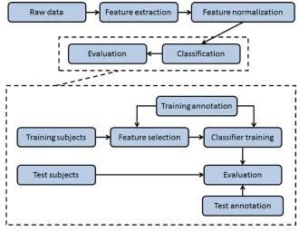
There are four main steps within the classification process, which are shown in Fig.2.2.
• Feature extraction. The goal of feature extraction is to extract relevant
informa-tion from the recordings. The distincinforma-tion between deep sleep and non-deep sleep
can hardly be seen from the raw sensor recordings. To better describes the
dif-ference between the two classes, a series of features are designed to extract the
characteristics from the recordings.
• Feature normalization. Features extracted from the raw recordings are further
processed to adapt to the requirements of the classifier, referred to as feature
nor-malization. Feature normalization helps to reduce the between-subject variability
in features. Thus, the performance of a generalized classifier is improved. The
classifier maps a set of normalized features to a class.
• Classifier training. During training, a classifier is tuned to a selected feature subset,
so that the generalization ability of the classifier is maximized. Feature selection
Figure 2.2: Flow-process diagram of the deep sleep classification framework.
• Performance evaluation. The training and evaluation of the classifier are performed
utilizing separate sets of subjects. Evaluation is usually done by splitting the
dataset in two, one is for classifier training and the other is for evaluation. In
practice, this method may suffer from lack of data. Therefore, we employ the
Leave-One-Subject-Out Cross-Validation (LOSOCV) paradigm for training and
evaluation, which will be explained in Chapter3.
2.3.1 Feature overview
Features are computed from the cardiorespiratory signals. Each feature describes a
characteristic of the cardiac and respiratory system. For example, the shapes of the
respiratory signals during deep sleep are more similar than those during the non-deep
sleep. Thus, a features expressing this characteristic would be a good candidate feature.
Though the sleep recordings are recorded at different sampling rates, features are
re-quired to describe each epoch with a single value, either an integer or a real number. The
computation of the features is usually restricted to a single epoch. For features which
describe the long-term change in cardiac and respiratory system, the computation will
not only consider the current epoch but also take the adjacent epochs into account.
0 1 2 3 4 5 6 7 50
55 60 65 70 75 80 85
Hours
[image:13.596.179.448.96.245.2]Mean heart rate
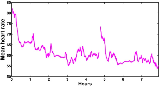
Figure 2.3: Mean heart rate over the entire night for one subject.
Two problems, which occurs frequently in features, are demonstrated in Fig.2.3: missing
values and trends in features. The missing values in features will cause problem for
those classifiers whose classification score is based on a linear combination of feature
values. Removing the epochs with missing values is not allowed since this will disrupt
the time series, and data coverage is decreased as well. To deal with the missing value
problem, cubic interpolation is employed. The values in epochs with invalid data are
interpolated according to the values of adjacent epochs. Since cubic interpolation aims at
interpolating using a smooth curve, it sometimes assigns extreme values for the missing
epochs (extreme values means that the assigned values far exceed the range of the
before-interpolation features). To avoid outliers in the after-before-interpolation features, only values
within the 2th percentile and 98th percentile of the total feature values are considered
as valid values. For those epochs whose values are outside the range, their values will
be set to the 2th percentile or the 98th percentile of the total feature values accordingly.
Trends in features is another problem since it is difficult for many classifiers to adapt
to the changes over time within the classifier itself. Thus, detrending is performed for
some features, most of them are features describing heart rate.
2.3.2 Cardiorespiratory features
This research utilizes many features which are claimed to be good at discriminating
deep sleep and non-deep sleep in literature. Thus, for each subject, 125 features are
computed. There are correlated features among the 125 features. Though the features
contain mutual information, they are still useful since they may carry unique information
that is good for classification but hard to isolated. Most features are ECG features, which
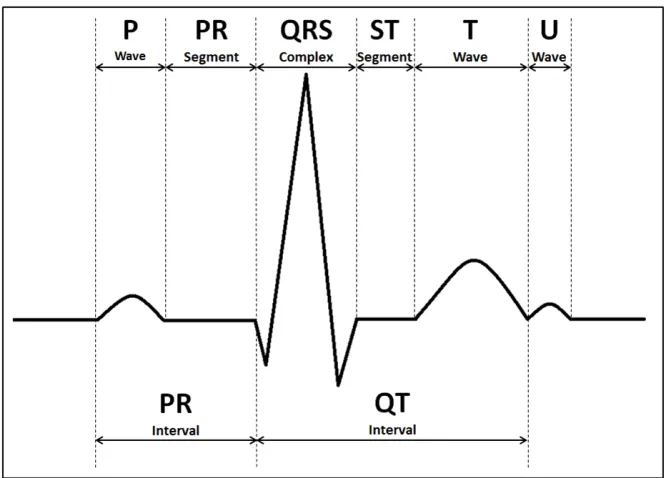
Figure 2.4: Schematic diagram of ECG waveform and attributes.
Since features are not the main focus of this research, we only provide a short description
of the most important features.
ECG features
To introduce ECG features, we first introduce ECG (Electrocardiogram) signal. ECG
interprets the electrical activity of the heart, which is generated by the polarization
and depolarization of cardiac tissue [32]. A single heartbeat ECG waveform and its
attributes are given in Fig.2.4. Features can be derived from RR interval, ECG-derived respiration (EDR) information and raw ECG signal.
RR interval represents the time between two successive R waves. It captures the
instan-taneous heart rate. Features derived from RR interval describe the heart rate variability.
Some example features, expressing the heart rate variability in the time domain, include
[33]:
• Mean of the normalized RR interval duration.
• Standard deviation of the normalized RR intervals.
• Range of RR intervals.
Features derived from RR interval in the frequency domain using power spectral density
(PSD) analysis. For cardiac analysis, three frequency bands are employed to the RR
(LF, 0.04-0.15 Hz) and High Frequency (HF, 0.15-0.45 Hz) [34]. The power in each of these frequency bands are shown to be good for discriminating deep sleep [35][31].
Another two types of ECG features that are proved to be useful for deep sleep
clas-sification employ detrended fluctuation analysis (DFA) and multiscale sample entropy
analysis respectively [36][37][38][39]. DFA eliminates trends in time series in order to study long-range correlations in the data. Multiscale sample entropy analysis
conduct-s a multi-conduct-scale (temporal and conduct-spatial conduct-scaleconduct-s) conduct-study to diconduct-scover the interactionconduct-s in the
physiologic systems.
Respiratory Features
Respiratory features measure the time domain as well as the frequency domain
informa-tion in the respiratory system. Similar to ECG signal, the extracted respiratory features
describe the respiration variability and contents in the same frequency bands (VLF,
LF and HF) as the cardiac features. In addition, some features related to respiration
amplitudes were extracted. Some important respiratory features are [40]:
• Standardized mean and median value of peaks and troughs of the respiration
am-plitudes.
• Median breath volume over time.
• Approximate entropy for peaks and troughs of the respiration amplitudes.
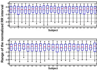
2.3.3 Feature normalization
Extracted features exhibit significant between-subject variability. For example, Fig.2.5
represents a box plot illustrating the distribution of a feature describing heart rate
vari-ability. Since this framework generates a generalized classifier, the generalized classifier
is obtained given various subjects. Such big between-subject variability makes the
gen-eralized classifiers difficult to achieve the optimal performance across the 45 subjects.
Its classification performance is limited by the variation between subjects. With the
feature in Fig.2.5, the generalized classifier is unable to find a constant threshold that
could achieve a good separation between two classes for all the subjects. Therefore,
features are normalized to eliminate the between-subject variability.
It is displayed in Fig.2.6 the normalized heart rate variability feature. The normal-ized feature of each subject is comparable. For each feature, one additional feature is
0 200 400 600 800 1000 1200
1 2 3 4 5 6 7 8 9 10 11 12 13 14 15 16 17 18 19 20 21 22 23 24
Subject
Range of the normalized RR interval
0 200 400 600 800 1000 1200
25 26 27 28 29 30 31 32 33 34 35 36 37 38 39 40 41 42 43 44 45
[image:16.596.135.480.115.364.2]Subject
Figure 2.5: Distribution of the heart rate variability feature of 45 subjects.
-3 -2.5 -2 -1.5 -1 -0.5 0
1 2 3 4 5 6 7 8 9 10 11 12 13 14 15 16 17 18 19 20 21 22 23 24
Subject
Range of the normalized RR interval
-3 -2.5 -2 -1.5 -1 -0.5 0
25 26 27 28 29 30 31 32 33 34 35 36 37 38 39 40 41 42 43 44 45
Subject
Figure 2.6: Distribution of the heart rate variability feature of 45 subjects after
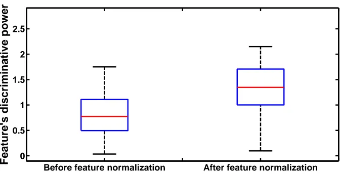
[image:16.596.137.478.452.705.2]Before feature normalization After feature normalization 0
0.5 1 1.5 2 2.5
[image:17.596.143.479.97.271.2]Feature's discriminative power
Figure 2.7: Distribution of the discriminative power of the heart rate variability
fea-ture among 45 subjects before and after feafea-ture normalization. Feafea-ture normalization improves the discriminative power of the original feature.
2.3.4 Classification
Classification includes feature selection and classifier training. Feature selection helps
to remove redundant information in features and improve the efficiency and efficacy for
the classifier. The classifier realizes the mapping between a set of features and classes.
Detail explanations of the classification process are in Chapter 3.
2.4
Initial results
This part summarizes the work of an early research investigation conducted prior to
this master project. The results of the early investigation are the initial results and
the conclusions drawn from the results motivate the work of this master project. The
work of the early investigation mainly targets on two tasks: one is to resolve the
class-imbalance problem in the dataset and the other is to test the performance of different
classifiers on deep sleep classification.
When introducing deep sleep, we have mentioned deep sleep only occupies 5 - 15% of total
sleep time. Therefore, in deep sleep classification, the positive class is the minority class.
In the dataset, on average, the ratio of the number of positive instances to the number
of negative instances is 1/7. Such a skewed data distribution makes the classification
problem even harder. The majority of the majority class are instances from N2 stage,
which is a stage that is the most easily been confused with deep sleep stage. The severe
results. Although there are more false negatives than false positives in the errors, the
harm of the false positives is bigger than the false negatives. In the introduction of
deep sleep, we have mentioned the stimulation should be given in accordance with the
progress of deep sleep. Otherwise, the stimulation will only interrupt the sleep process.
These false positives make the timing of stimulation inaccurate. Therefore, solving the
class-imbalance problem in the dataset is one major task of the early investigation.
We approached the imbalance problem from the data level. One can also think of solving
the imbalance problem from the algorithm level. On the algorithm level, the technique
is called cost-sensitive learning, which is to introduce a cost matrix to describe the
cost of misclassification in order to compensate and/or penalize the misclassification
of minority class instances and majority class instances. In our case, the objective of
solving the class-imbalance problem is to achieve a balanced data distribution. The
reason we approach the class-imbalance problem from the data level is that the classifier
used for deep sleep classification in this framework can be considered as solving the
class-imbalance problem from the algorithm level. The trained classifier models each
class separately, implicitly achieving the goal to ignore the percentage of data for each
class in the dataset. We therefore adopted methods from the data level as another way
to solve the problem.
On the data level, the objective is to achieve a balanced data distribution in the training
set. Thus, the trained classifier will not be biased in favor of the majority class. The
re-sampling technique we adopted is down-re-sampling the instances from the majority class.
Up-sampling the instances from the minority class is another way to achieve a balanced
data distribution. However, up-sampling results in more instances for training, therefore
overload the training system with more calculations. Two down-sampling techniques
have been employed, one is random down-sampling the instances from majority class,
another is informative sampling the instances from majority class. Random
down-sampling method is simple. It randomly selects a part of instances from the majority
class, to make sure in the training data, the number of instances from the majority class is
the same as the number of instances from the minority class. Informative down-sampling
method is more complex. The instances from the majority class sampled by it are those
instances which are called the representative instances. The representative instances are
the majority instances that are difficult to differentiate from the minority instances. The
training set, which is comprised of the minority instances and the representative majority
instances, makes the trained classifier learn the difference between these hard-to-classify
instances.
trained on the obtained training set. The obtained training sets are trained with a
k-Nearest Neighbor (kNN) classifier, and then tested on the test set. The choice for the
kNN classifier is motivated by its simplicity. kNN classifier suffers greatly if the training
data has severe class-imbalance issue. Therefore, it is appropriate to evaluate the quality
of the re-sampling techniques. The performance of the kNN classifier is compared with
the performance of a linear discriminant (LD) classifier. The LD classifier is trained
on the original training set (which is not re-sampled). The impact of skewed data
distribution on a LD classifier is small. The goodness of a LD classifier depends on
the extent to which the data meets the assumptions of linear discriminant. Although
it holds the assumption of shared covariance matrix, in practice, it can achieve good
performance as long as both classes approximate Gaussian distribution even for skewed
data distribution. Although we proposed a way to deal with the class imbalance problem
in the dataset, the simple LD classifier still performed the best on the classification task.
Although the informative re-sampling technique helps to preserve the representative
ma-jority instances and make the amount of both classes comparable, the re-sampled data
still exhibits highly degree of mixture between classes, which makes the classification
problem still difficult. Thus, the conclusions we drawn are it is easy to achieve a
bal-anced data distribution with re-sampling techniques but it is extremely difficult to get
a classifier with the re-sampled data who can perform better than a classifier immune
to skewed data distribution.
Since resolving the class-imbalance problem is unable to give a better classifier, we
switched the work to test the performance of different classifiers on deep sleep
classi-fication. We have experimented with linear classifier and non-linear classifier. After
comparing their performance, linear discriminant (LD) turned out to outperform other
classifier on deep sleep classification. Classifiers which takes context into account might
perform better in deep sleep classification since sleep exhibits dependence between stages.
For example, some use Hidden Markov Model in sleep staging [41][42][43]. Nevertheless, we restricted our test to classifiers who do not try to model the relationship between
instances. Under such circumstances that the best classifier for deep sleep classification
is LD.
After examining the classification results, we have noticed some issues. When we put
the classification results and the hypnogram of the test subject together, we found there
might be a connection between the classification result and characteristics of the deep
sleep. Fig.2.8 illustrates hypnograms of two subjects and corresponding classification results. By looking at Fig.2.8(a) and Fig.2.8(b), we have a rough impression that the
classification performance might be related to the continuity of deep sleep. The
0 1 2 3 4 5 6 7 8 N3
N2 N1 REM Wake
Hours
0 0.1 0.2 0.3 0.4 0.5 0.6 0.7 0.8 0.9 1
0 0.5 1
Recall
Precision AUC-PR = 0.95
(a) Hypnogram and classification result of subjecta.
0 1 2 3 4 5 6 7 8
N3 N2 N1 REM Wake
Hours
0 0.1 0.2 0.3 0.4 0.5 0.6 0.7 0.8 0.9 1
0 0.5 1
Recall
Precision
AUC-PR = 0.47
(b) Hypnogram and classification result of subjectb.
Figure 2.8: Examples of two hypnograms and corresponding classification results. N3
is the deep sleep stage. Classification result is given by thePrecision-Recall curve and area under thePrecision-Recall curve (AUC-PR).
stages. The performance of subject b is worse and his/her sleep has been interrupted
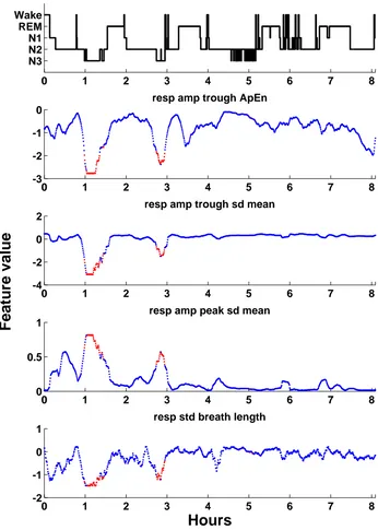
by other stages frequently. Fig.2.9shows a hypnogram and four features of a subject.
Both of these features are with strong discriminative power for deep sleep classification
for the subject. The deep sleep in the first half of the night is more continuous than
those in the second half of the night. And in the feature plots, the difference between
positive epochs and negative epochs in the first half of the night is obvious while it
is difficult to differentiate between positive epochs and negative epochs in the second
0 1 2 3 4 5 6 7 8 N3
N2 N1 REM Wake
0 1 2 3 4 5 6 7 8
-3 -2 -1 0
Feature value
resp amp trough ApEn
0 1 2 3 4 5 6 7 8
-4 -2 0 2
resp amp trough sd mean
0 1 2 3 4 5 6 7 8
0 0.5 1
resp amp peak sd mean
0 1 2 3 4 5 6 7 8
-2 -1 0 1
[image:21.596.131.477.146.631.2]Hours
resp std breath lengthFigure 2.9: An example of hypnogram and features. Feature names are indicated
deep sleep interval. This property that may have impact on the performance of deep
sleep classification is not encoded in the features but is the characteristic of the deep
sleep interval itself. There might be other factors which may also affect the deep sleep
classification, such as the age of the subject and the duration of deep sleep intervals.
Therefore, we suspect that the performance of deep sleep classification is affected by the
characteristics of deep sleep and the subjects, which is the first hypothesis that needs
to be validated.
Another issue is the limitation of the subject-independent model. Though the
perfor-mance of the subject-independent model is good in general, its perforperfor-mance on specific
subjects can be low. Instead of blaming the classifier, we turned the attention to the
features. It is observed that the selected features, which have strong discriminative
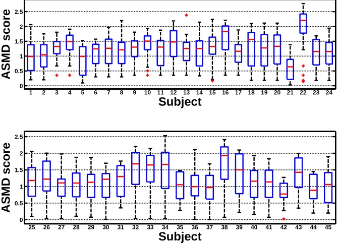
pow-er ovpow-er all, behave badly for specific subjects. Fig.2.10illustrates the distribution of the
discriminative power (ASMD scores) of the selected features for each subject. It is clear
that the range of scores varies significantly between subjects. The subject-independent
model, which is not tailored to specific subjects, is unable to discover what is the real
good features for them (By real good features, we mean features with strong
discrimina-tive power.). In other words, the subject-independent property of the constructed model
limits its ability on accounting for the personal characteristics in features. Therefore, the
second hypothesis is formed, which is for a specific subject, a personalized model is able
to provide better performance on deep sleep classification than a subject-independent
model.
So far, the two hypotheses, which are motivated by the work done before the master
project, are stated and will be validated in the following chapters. The validation of
the two hypotheses will provide new directions for the research work on improving the
performance of deep sleep classification using features derived from cardiorespiratory
signals.
Hypothesis I:
The performance of deep sleep classification is affected by sleep
characteris-tics which are not captured in features.
Hypothesis II:
Personalized classifier can help improve the performance of deep sleep
0 0.5 1 1.5 2 2.5
1 2 3 4 5 6 7 8 9 10 11 12 13 14 15 16 17 18 19 20 21 22 23 24
Subject
ASMD score
0 0.5 1 1.5 2 2.5
25 26 27 28 29 30 31 32 33 34 35 36 37 38 39 40 41 42 43 44 45
Subject
[image:23.596.145.481.289.533.2]ASMD score
Figure 2.10: Distribution of the discriminative power (ASMD scores) of the selected
Methods
In Chapter 2, two hypotheses have been presented, which will be validated in this re-search. These two hypotheses mention two aspects that may influence the performance
of deep sleep classification. The first hypothesis states the relationships between
classifi-cation performance and one sleep characteristic or a series of sleep characteristics which
are not encoded in features. The second hypothesis focuses on the importance of
per-sonalization of deep sleep classifier. In this chapter, methods and steps for hypotheses
validation are explained. The dataset used in the research is also introduced in this
chapter.
3.1
Experimental setup and Dataset
Experimental Setup
The dataset used in this research is from the sleep database created during the EU Siesta
project (1997-2000) [44]. This project was organized as a multi-center study, which comprised 8 clinical partners and 8 engineering groups located in Europe. In current
study, the dataset is comprised of recordings from 7 separate labs. Each subject spent
two consecutive nights in the same sleep lab using the same sensors. Different sensors
were used in different labs, therefore variation in the recordings between subjects caused
by varying sensors readings are to be expected.
For each subject, lead II ECG configuration was used on the chest to acquire ECG
signals. The respiratory effort signal is obtained by measuring the chest circumference
using respiratory inductance plethysmography.
Dataset
M ean±std Range Age 43.6±17.1 20 - 86 Time in bed (hours) 7.9±0.4 6.7 - 9.3
Sleep efficiency (%) 84.7±6.5 73.9 - 97.5 Deep sleep (%) 14.2±4.4 6.7 - 24.8
Wake (%) 15.4±6.5 2.5 - 26.1 REM (%) 16.8±3.5 10.8 - 26.3 30 female subjects and 15 male subjects.
Table 3.1: Population statistics among the 45 subjects
The dataset includes recordings of 45 subjects two-night sleep. Subjects are selected for
their healthy sleep patterns and high data coverage. Subjects those do not exhibit a
healthy sleep pattern are excluded from the dataset. Healthy subjects whose recordings
have missing values of more than 50 continuous epochs are excluded. None of the 45
subjects have known sleep disorders. For the purpose of hypothesis validation,
origi-nal recordings are segmented into sleep cycles. The first-night recordings after cycle
segmentation of the 45 subjects are used in the validation of the first hypothesis. The
validation of the second hypothesis utilizes both nights recordings of the 45 subjects. 13
subjects are selected from the 45 subjects, whose both nights recordings are segmented
into cycles for the validation of the second hypothesis as well. The selection criteria for
the 13 subjects are explained later in the chapter. The validation of the two hypotheses
will be the guidance for the future work on improving the performance of deep sleep
classification using features derived from cardiorespiratory signals. An overview of the
demographics and sleep statistics of the first-night recordings of the 45 subjects is given
in Table.3.1.
3.2
Hypothesis 1 validation: Regression analysis
The first hypothesis that needs to be validated is: performance of deep sleep
classifica-tion is affected by sleep characteristics which are not captured in features. These sleep
characteristics are called inf luencial f actors. Regression analysis is chosen to validate
the first hypothesis since it is a statistical approach in order to investigate the
relation-ship among a set of variables. It is used to model and analyze the relationrelation-ship between
response variable (Y, also called dependent variable) and explanatory variables (Xis,
also called independent variables), which helps to understand how the response variable
changes when any of the explanatory variables varies. In our case, the response variable
is the classification performance and the explanatory variables areinf luencial f actors.
Linear regression is the easiest category of regression analysis [5]. This is because the assumed linearity among variables makes the model easy to fit and the statistical
prop-erties of the estimated parameters are easy to interpret. The constructed model is a
linear combination of explanatory variables in order to predict the outcome of response
variable. Linear regression could also be used to quantify the strength of the
relation-ship betweenY andXis. It reveals whichXi has a stronger impact onY and whichXi
has little impact on Y. The model could have one explanatory variable, the case which
is called simple linear regression, or multiple explanatory variables, the case which is
called multiple linear regression. In later discussion, we are focusing on multiple linear
regression.
To determine whether it is appropriate to use linear regression modeling the data, it
is essential to plot the data first. Scatter plots are recommended to determine the
relationship among variables. If the variables appear to be linearly related, a linear
regression model can be used then. If the variables are not linearly related, one can
tackle the problem by transforming the data or adopting a non-linear model to establish
the relationship among variables.
3.2.1 Equation and parameter estimation
Linear regression assumes the relationship betweenY andXis is linear. Given a data set
{Y, x1, x2,...,xn−1, xn}, Y is defined as response variable or dependent variable while xis are defined as explanatory variables or independent variables. In linear regression,
the simplest relationship betweenY and Xi can be modelled as:
Y = X
1≤i≤n
βixi+b+ε,
where βi is the linear coefficient corresponding to xi, and ε is the error term, which
denotes for the unobserved random variable which adds noise to the model. Such model
poses a big advantage in terms of interpretability, however can be over simplistic in some
cases. In this thesis, a more flexible linear regression model that allows between-variable
interaction is adopted:
Y = X
1≤i≤n βixi+
X
1≤i,j≤n
γi,jxixj +ε,
where γi,j models the influence of theinteraction term xixj on response variable. The
interaction term xixj assumes that the independent variable xi(xj) has a effect on Y
depending on the values of the independent variablexj(xi). This model, called the
scenarios. The two-way interaction model can be further extended to a more generic
and flexible form, allowing more interactions among variables, e.g., three-way linear
regression model. As interpretability comes as an expense of flexibility, we restrict the
discussion within the scope of two-way linear regression.
In order to estimate coefficients of independent variables, ordinary least squares (OLS)
is employed. This method minimizes the sum of squared vertical distances between the
response variables in the dataset and the response variables predicted by the model.
Assume the response variable in the dataset is Y and the response variable predicted
by the model is Yf it, OLS attempts to estimate unknown parameter by minimizing
Σ(Y −Yf it)2. (Y−Yf it) is also called residual, thus OLS attempts to estimate unknown
parameters in the linear regression model by minimizing the sum of squared residuals.
Assumptions
In order to validate the use of linear regression model, a series of assumptions should
be met by the variables. If the assumptions are violated, then the results are not
trustworthy. According to [45], the assumptions are:
• The measurement of dependent variable and independent variables is error free.
• Dependent variable and independent variables are linearly related.
• The independent variables should be independent of each other.
• Dependent variable should be normally distributed given each value of the
inde-pendent variables.
• The variance of the residuals is constant for all values of the independent variables,
dependent variables and fitted values of the dependent variables
(homoscedastici-ty).
• The residuals are independent of each other.
• The residuals should be normally distributed.
Among these assumptions, the first four assumptions should be met by the data and
the last three assumptions should be met by the residuals. The assumptions can be
summarized as: independence, linearity, normality and homoscedasticity. To validate
a linear regression model, the residuals of the model should be normally and randomly
3.2.2 Evaluation of a linear regression model
Evaluation of a linear regression model consists of evaluating whether the assumptions
of linear regression are violated and the adequacy of the model.
Residual analysis is used to check for the assumptions. To check for normality, a
quantile-quantile plot (Q-Q plot) can be used. Q-Q plot is used to compare two probability
distributions [46]. If the two distributions being compared are similar, the points in the Q-Q plot should approximately lie on the line y = x. In order to check whether
the residuals are normally distributed, the y-axis has been fixed with quantiles from
a normal distribution with mean 0 and standard deviation 1. The modified Q-Q plot
is called normal probability plot. By examining the deviation from the line y = x in
the normal probability plot, one can check for the normality of residuals from a linear
regression model.
To check for linearity and homoscedasticity, one could produce a scatter plot, plotting
residuals against predicted response variable. Ideally, residuals are randomly scattered
around 0 and have a relatively even distribution, exhibiting a shape resembling centrally
dense cloud. To quantitatively test for the homoscedasticity, one can use a
Breusch-Pagan test [47]. It is a test for heteroscedasticity in a linear regression model. It can
detect whether the heteroscedasticity in a linear regression model comes from the linear
dependence between the residuals and the independent variables in the model.
Breusch-Pagan test employs OLS to construct a regression model for the squared residuals with
a linear combinations of the independent variables. The hypothesis of
homoscedastic-ity can be rejected when an F-test suggests that the regression model is statistically
significant.
Some statistical properties are derived to assess the goodness-of-fit of a linear regression
model [5]. Typically, people use R-square and/or adjusted R-square, root mean squared error (RMSE) and marginal sums of squares (Type III SS) to test whether the fitted
model is good. R-square measures how many variances in the dependent variable has
been explained by the fitted model. Values of R-square are in the range 0 to 1. R-square
= 1 indicates that the fitted model accounts for all variances in the response variable.
Thus, R-square is desired to be as high as possible. However, a high R-square does
not necessarily indicate that the model has a good fit. R-square alone does not tell the
entire story. In order to have a comprehensive view of the constructed model, R-square
values as well as residual plots and other model statistics should be evaluated. When
the model has many explanatory variables, one may use adjusted R-square instead.
variables. Adjusted R-square takes into account the number of explanatory variables
when calculating. Thus adjusted R-square is always lower than R-square.
Root mean squared error (RMSE) measures the difference between estimated values of
response variables and true values of response variables. RMSE is desired to be small,
meaning the predicted values of response variable are close to the true value of response
variable.
Type III SS measures the sum of squares in the error which can be obtained for each
explanatory variable if it was the last variable entering the model. The effect of each
variable is evaluated after all other variables have been considered. The goal of this
metric is to test the significance of each independent variable in the fitted model. A
variable is considered statistically significant when it has a Type III SS p-value of 0.05
or less.
3.3
Hypothesis 2 validation
The second hypothesis which will be validated in the research is: personalized classifier
can improve the performance of deep sleep classification. The experiment procedures
for validating the second hypothesis are explained in this part. A thorough description
of the methods for feature selection and classifier is also given in this part.
3.3.1 Classification
As mentioned in Chapter2, classification includes feature selection and classifier training. The feature selection method employed in the framework is explained as well as the
classifier trained for deep sleep classification.
Feature selection
The goal of feature selection is to select a feature subset from original feature space
in order to build a classification model afterwards. The objective of feature selection
is to reduce the amount of redundant features and irrelevant features in the feature
s-pace. Having many redundant features will cause overfitting problem for the constructed
model. The constructed model will have difficulty in generalizing to new, unseen data
if it has been trained with too many equal examples of the same thing, while irrelevant
features will not contribute to the constructed model. Therefore, feature selection is
expected to tackle these two problems. Moreover, feature selection helps to identify key
Since feature selection reduce the amount of features used in model construction, both
the training time and test time will be reduced.
Feature selection method could be sorted into two broad types: filter methods and
wrapper methods. Both methods attempt to find one feature subset which contributes
most according to some evaluation metrics. Filter methods measure the “usefulness”
of features, such as the mutual information between features, the correlation between
features etc. Therefore, feature subset selected by filter methods is not tuned to a
specific classification model. Wrapper methods use a classification model to score feature
subsets based on their performance on a given test set. Since wrapper methods consider
the interaction between the classification model and the training set, it is thought to
achieve the best possible performance with a particular learning algorithm on a particular
training set. However, wrapper methods could not guarantee the selected subset is the
best in terms of generalization since overfitting problem might occur in some cases
[48][49].
Since for each candidate feature subset, wrapper methods need a model to be trained,
it is a computational intensive task. Moreover, we are interested in not only the
per-formance of selected feature subset on the given dataset with a particular classification
model but also the quality of features. Hence we adopt filter methods for their simpler
computational methods and better generalization ability [50].
Correlation Feature Selection
Correlation Feature Selection (CFS) [51] is a supervised feature selection method which makes use of the ground-truths of training examples in the selection process. The
hy-pothesis adopted by CFS is that good feature subsets should contain features that are
highly correlated with ground-truths while the correlations between features are weak.
The merit of each feature subset is calculated as:
M eritS=
k·corr(c, S)
p
k+k(k−1)corr(S, S),
wherec is the ground-truths of the features in set S and k is the number of features in
S. corr(c, S) is the correlation between the features in set S and c. corr(S, S) is the
average pairwise correlation between features in S. The correlation is defined by the
Pearson’s linear correlation coefficient. Different search algorithms could be used, such
as forward search or backward search, to find the feature subset with the highest merit.
CF S= arg max
S M eritS.
Classifier assigns an instance to a category (class) according to its characteristics.
Char-acteristics will be represented by a series offeatures. The objective of classifier is to find
a mapping betweenfeatures and class labels. A classifier can handle binary class
classi-fication problem as well as multi-class classiclassi-fication problem. The classiclassi-fication problem
in this research is a binary class problem which decides whether an instance belongs
to deep sleep or non-deep sleep. Many classifiers have been investigated and achieve
varying degrees of success in sleep stage analysis [52][53]. Some used simple classifiers,
such as linear discriminant classifier, while some used more complex classifiers, such as
neural network. Simple classifiers are easier to interpret and implement but they might
not be able to learn all the useful information from the data. Complex classifier may well
model the data but when the data is limited it will probably cause overfitting problem
[54][55]. In this research, linear discriminant classifier is utilized.
Linear Discriminant
Linear Discriminant classifier (LD) is a simple and robust classifier. It was first
intro-duced by Fisher [56]. LD classifier attempts to construct a function which is a weighted combination of features. Hence the decision boundary drawn by LD is a hyperplane in
a high-dimensional feature space. LD assumes that each instance is generated from a
multi-variate Gaussian distribution and the covariance matrix of each class is the same.
Though in many real-life cases these two assumptions are violated, it also performs well
in those cases.
The aim of LD classifier is to find a hyperplane that maximally separates two classes. The
output of LD classifier is a numerical value which could be interpreted as the difference
in standardized distances between the two classes. An instance will be assigned to the
class that is closest to it. LD classifier uses probability to measure the distance between
an instance and classes.
Given two classes p and n, indicating positive and negative class respectively, and an
instance x with unknown label, the task is to find the most probable class that this
instance belongs to. This can be achieved by comparing the posterior probability of
P(p|x) and P(n|x):
y=P(p|x)−P(n|x).
If y is greater thanT, then the instance x will be assigned to positive class, otherwise
it will be assigned to negative class. T then is a threshold for the scores given by LD
classifier that can be manually set, which makes the classifier more flexible in order to
achieve a better performance towards the priority class (in our case, deep sleep is the
Directly computing y is difficult since it needs to model posterior probability. But
with Bayes theorem, posterior probability can be expressed by prior probability and
likelihood:
P(p|x) = P(x|p)P(p)
P(x) , P(n|x) =
P(x|n)P(n)
P(x) .
y is therefore expressed as:
y= P(x|p)P(p)−P(x|n)P(n)
P(x) .
Prior probability can be easily computed as the number of times instances belonging
to one class against the number of all instances. With LD classifier’s two assumptions,
likelihood can also be computed. We denote the Gaussian distribution of the positive
class befp∼N(µp,Σ), whose mean isµpand covariance matrix being shared covariance
matrix Σ. And the Gaussian distribution of the negative class befn∼N(µn,Σ), whose
mean is µn and covariance matrix being shared covariance matrix Σ. Thus, likelihood
of P(x|p) is:
P(x|p) = p 1
(2π)k|Σ|exp(−
1
2(x−µp)
TΣ−1(x−µ
p)),
wherek denotesx haskfeatures. P(x|n) can be expressed likewise.
When computingy, bothP(x) and the part outside of the exponential of likelihood can
be left out because they will not contribute to the final score since they are constant
terms over two classes. To simplify computing, we take the natural logarithm ofy, then
we have:
y=logP(x|p)−logP(x|n) +logP(p) P(n),
y=−1
2(x−µp)
TΣ−1(x−µ
p) +
1
2(x−µn)
TΣ−1(x−µ
n) +log P(p)
P(n).
y is the score function of LD classifier. If we set the threshold to T, then LD classifier
draws a decision boundary through the feature space along y = T. Note the prior
probability could be manually set when the distribution of two classes are imbalanced in
order to give more weights to minority class, which achieves the same effect as changing
the value ofT.
3.3.2 Experiment procedure
To validate the second hypothesis, we have designed several experiments to compare
the performance of the personalized classifier and the subject-independent classifier.
Because we have recordings of two-night sleep for 45 subject, the first experiment is to
M ean±std Range Age 39.8±14.8 20 - 71 Time in bed (epochs) 941.6±43.3 799 - 989
Sleep efficiency (%) 89.7±5.2 81.6 - 97.5 Deep sleep (%) 16.5±4.6 7.1 - 28.0
Wake (%) 10.3±5.2 2.5 - 18.4 REM (%) 20.0±4.3 12.2 - 29.2 10 female subjects and 3 male subjects.
Table 3.2: Population statistics among the 13 subjects
classifier evaluation. The second experiment is to compare the performance of classifiers
trained with segmented data. In the second experiment, subjects’ data are segmented
into sleep cycles. The purpose of cycle segmentation is to overcome the lack of training
data problem. To ensure the validity of the experiments using cycles, the first step
is to make a selection of subjects. This is step is to ensure the sleep characteristics
variability between nights is not high within one subject. Sleep characteristics is defined
as the percentage of different sleep stages, number of cycles, and duration of sleep.
Each percentage of the characteristics of the selected subject between the two nights
does not differ by more than 20%. Based on the criteria, only 13 subjects are selected
from the 45 subjects. The validation of the hypothesis will prove the feasibility of
constructing a personalized classifier which can therefore improve the performance of
deep sleep classification. An overview of the demographics and sleep statistics of the
13 subjects is given in Table.3.2. Due to the limited number of selected subjects, the experiment is only a pilot study of personalized classifier on deep sleep classification.
Cycle segmentation
After subjects selection, we can proceed to cycle segmentation. The first cycle is between
the sleep onset and the end of the first REM period. The subsequent cycles are defined
between the end of REM sleep of the previous cycle and the next end of REM sleep.
A REM period briefly interrupted by micro-arousals can be tolerated. If there is an
awakening, which lasts for longer than 5 minutes, in the middle of a cycle, then the
cycle is interrupted by this event. Each of the 13 selected subjects has 6−12 sleep
cycles. Sleep cycles without deep sleep stage are excluded. Thus each subject has 3−6
valid sleep cycles.
3.3.3 Evaluation of hypothesis 2
d = 1
d = 3 d = 2
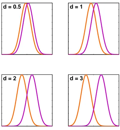
[image:34.596.220.421.104.322.2]d = 0.5
Figure 3.1: Gaussian densities illustrating various values of Cohen’sd(ASMD)
3.3.3.1 Feature evaluation
Two metrics are adopted to evaluate the effectiveness of a feature: absolute standardized
mean difference (ASMD) and area under the Precision-Recall curve (AUCPR).
Absolute Standardized Mean Difference
Absolute standardized mean difference (ASMD) is a measurement of the discriminative
power of a feature between two classes. This metric is a variation of standardized mean
difference, Cohen’sd[57]. Cohen’sdis a measurement for effect size based on distances
between means of different groups. Since the magnitude of Cohen’s d is of interest in
this research, we useASMD instead.
For a feature f, its ASMD is calculated as the absolute difference in the mean of two
classes divided by the pooled standard deviation for both classes
ASM D(f) = |µp−µn|
σ ,
here µp and µn are the means of positive class and negative class in f, and σ is the
standard deviation for f over two classes. Since we assume both classes are normally
distributed, Figure3.1illustrates various values of Cohen’s d(ASMD). It could be seen
from the plot that a feature with a largerASMD value has a higher discriminative power
d=0.2; medium,d=0.5; and large,d=0.8. Therefore, we decide that if theASMD value
of a feature is larger than 1 then the discriminative power of the feature is strong, while
the smaller than 0.5 ASMD value means a feature with weak discriminative power in
separating two classes.
Area under the Precision-Recall curve
Precision-Recall curve is a visualization tool to examine classification performance,
es-pecially when there is class-imbalanced problem [58]. Precision-Recall curve and area
under the Precision-Recall curve (AUCPR) are usually adopted to evaluate the
perfor-mance of classifier. The construction of Precision-Recall curve requires classification to
be done first. However, these metrics could also be used for evaluating features. As
mentioned before, when a thresholdT is set for the score function of a LD classifier, the
binary classification result for the test set can be obtained. With varying T, a series
of classification results can be obtained. Thus a series of precisions andrecalls can be
derived to make thePrecision-Recall curve. If we want to make aPrecision-Recall curve
for a featuref, we only need to replace the classification score by the feature value off
since the feature value is numerical. Then we could have the same process of
construct-ingPrecision-Recall curve for a classifier to get thePrecision-Recall curve for a feature.
Details of Precision-Recall curve will be explained later in the chapter.
3.3.3.2 Classification evaluation
Classification performance could be used to evaluate a classifier and/or a selected feature
subset. The dataset is split into training set which a classifier is built on and test set
which is used for the performance evaluation for the trained classifier.
Cross-Validation
Usually we split the dataset into training set and test set for classifier modeling and
evaluation. However, this approach is not appropriate in this research since we only
have a dataset of 45 subjects. In order to test the classifier on as large as possible
test set, while keeping the training set also large and independent of the test set, we
consider cross-validation. Cross-validation does not need an independent test set. It
partitions the current dataset, on the subject basis, into two disjoint subsets: one is
used for training a classifier, whereas the other is used to evaluate the classifier. This
procedure is repeated until all subjects in the initial set have been tested.
We applied the Leave-One-Subject-Out cross-validation (LOSOCV) scheme which is a
special case of cross-validation where the test set consists of data from only one subject
individually trained classifiers, each one followed by a test run. Results are reported by
the averaged performance over the 45 classifiers.
Performance Measure
To evaluate the performance of a classifier and compare the performance between
d-ifferent classifiers, we need to make a choice for performance measurement. Accuracy
or error rate is normally used in performance measurement. However, high accuracy
does not necessarily imply better performance on target task, particularly there is a
class-imbalanced problem. When the data distribution is imbalanced, accuracy will be
biased in favour of the majority class. Since the classification problem in this research
is a binary case, the explanations of the performance measurement will be restricted to
the two-class case.
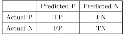
With a score given by the LD classifier and the threshold T, each test instance will
receive a label of either Positive (P) indicating it is deep-sleep or Negative (N) indicating
it is non-deep sleep. Given its original label and the classification result, there are four
possible outcomes for each test instance:
• True Positive (TP): The original label of the instance is positive and the classifier
correctly labels it positive.
• True Negative (TN): The original label of the instance is negative and the classifier
correctly labels it negative.
• False Positive (FP): The original label of the instance is negative and the classifier
erroneously labels it positive.
• False Negative (FN): The original label of the instance is positive and the classifier
erroneously labels it negative.
These possible outcomes are usually shown in what is called a confusion matrix. The
structure of a confusion matrix is shown in Table3.3.
Predicted P Predicted N
Actual P TP FN
[image:36.596.216.414.614.671.2]Actual N FP TN
Table 3.3: Example of confusion matrix
Several statistics can be derived from the confusion matrix: