Decay functions in commodity freight flow models A regression model for deriving the decay parameter

Full text

(1)Decay functions in commodity freight flow models A regression model for deriving the decay parameter. Author: Adrianus J. Mulder Date: October 14, 2011 Student ID: S0089621 Academic Institution: University of Twente Industrial Engineering and Management – Production and Logistics First internal supervisor: Dr. P.C. Schuur Second internal supervisor: Dr. ir. L.L.M. van der Wegen Employer: Centre for Supply Chain Management – Stellenbosch University External supervisor: Dr. J.H. Havenga.

(2)

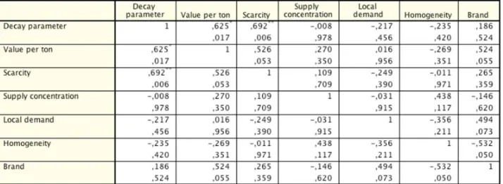
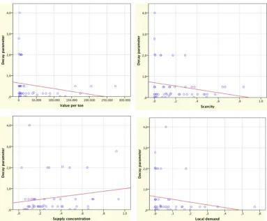
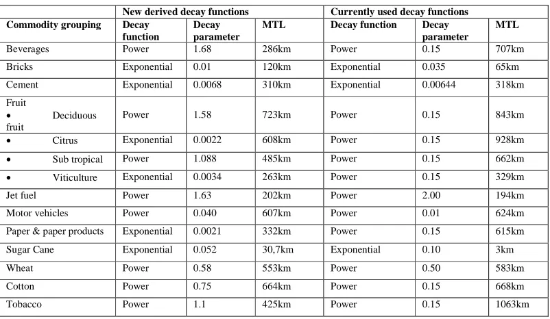
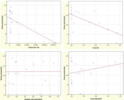
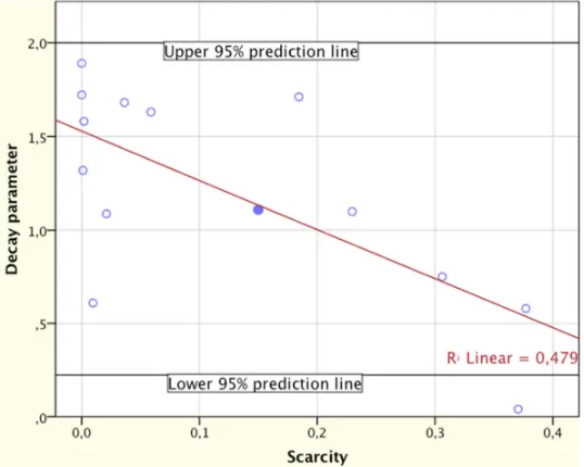
(3) Management summary Since 2006 South Africa has her own commodity freight flow model in place that is aiming to predict the freight flows for all goods in the country (aggregated in 64 commodity groupings) up to 30 years into the future. The model is based on gravity modelling; a technique that models the interaction (freight flows) between supply and demand points based on their size and the resistance (for example distance) between them. An important component in this model, the decay function, describes the decay in volume transported over an increasing resistance variable (distance, time or cost). In general a negative power function or negative exponential function is used. The exponent of the function, the decay parameter, varies for different commodity groupings. It is high for products that are only transported over short distance and low for products that are transported over long distance. Normally the decay function and its parameter are derived from actual freight flow data obtained from a statistical bureau, a logistical survey or a census. However as no obligation exists for companies in South Africa to hand over freight flow data and the other methods have not yet been carried out in South Africa as they are very costly and time consuming to perform, the current decay functions have been established based on a trial-and-error, lacking scientific background. Goal of this research has been to develop an alternative way to provide scientific background for and improve the use of the currently applied decay functions for transport by road in South Africa. The method used is based on regression modelling and assumes that the level of decay can be predicted by an (combination of) other factor(s). Six different factors that were expected to influence decay have been tested in correlation analyses: ‘Value per ton’, ‘Scarcity’, ‘Supply concentration’, ‘Local demand’, ‘Homogeneity’ and ‘Brand’. The decay in these analyses has been represented by the parameters of negative power decay functions. These functions were derived from actual freight flow data related to 14 different commodity groupings, which were selected based on the amount of gathered freight flow data from industry. This resulted therefore in 14 observations (decay parameter values) for the correlation analyses. From the expected relationships between the different factors and decay only ‘Scarcity’ was moderately correlated with decay. The relationships with the rest of the factors were mostly weak and insignificant. ‘Scarcity’ was therefore the only explanatory variable included in the regression model resulting in the following regression model expression: Decay parameter = 1.528 -2.628 Scarcity The explanatory value of this regression model (R2) is 0.479 at a significance level of 0.05. Even at a significance level of 0.003 the relation between ‘Scarcity’ and decay is expected to be negative. Because of doubtful data and remarkable differences with the outcome of other studies it is suggested to exclude the commodity grouping ‘Bricks’ from the regression analysis. This would lead to an increase of R2 to 0.681 with an observed significance level of less than 0.001. As no verification data are available it is hard to quantify the quality of the model. Given the 95% prediction intervals the accuracy of the model is not very high. Therefore the model can only be used as an indication for the decay parameter value. i.

(4) Many factors have or may have influenced the correlation and regression analyses. Especially the level of detail (size of the regions), selection of commodity groupings, amount and quality of the obtained data and the processing of the data have had their impact on the values of the decay parameters and scores of the possible influencing factors. Besides the issues with data and methodology also the different time frames (1967 vs. 2010) and countries (US and Europe vs. South Africa) will have influenced the comparison between the studies, the value of the derived decay parameters and their relationships with the possible influencing factors. The correlation analyses and comparison with similar studies should therefore be made and interpreted with caution.. ii.

(5) Preface My choice for the assignment was in the beginning solely based on my wish to visit South Africa and experience the country, I fell in love with while travelling, in a different context. However the more I learned about the subject and the influence it has on the logistical developments in South Africa the more interested I became and in the end I spent more weekends figuring out the freight flows in South Africa than I enjoyed her wines and braais (barbeques). Almost turning work into a hobby. Carrying out my thesis abroad has given some extra challenges in guidance from and communication with my home university but it has on the other hand improved my independence. The whole experience has broadened my horizon academically as well as cultural and social. When I left South Africa I left a beautiful country, a great group of friends and my second home. All in all an opportunity I have to thank both my internal as well as my external supervisors for. I also want to thank the whole team at the Centre for Supply Chain Management that first of all invited me in their office and gave me a very warm welcome. They always made time to discuss my hypotheses and answer my questions, gave useful advises on different topics and even grabbed the phone to support me in my quest for actual freight flows. Special thanks are directed to my dear mother who took the time to go through the whole report and was able to point out the obstacles for readers inexperienced with the topic. It has definitely added to the readability of the report. Yvonne definitely deserves my appreciation for all her help and support. She has been a wonderful friend that always knew how to motivate me but also remind me to place issues regarding my assignment in perspective whenever necessary. Finally I have to apologize to the contact persons of the different companies that I have called so often to remind them about my request for information that the secretaries started to remember my name. I believe that although the result of the project might not fully support the initial desired outcome, it has given different useful insights in South African freight flows, resulted in several useful data sets with actual freight flows and a long list of relevant contact persons in the industry. The invitation from the Centre to stay and perform a PhD project was the best appreciation I could receive. I hope this project will lead to more cooperation between both universities in the future, as there is still a lot to learn from each other. I am aware of the fact that eighty pages seems a lot but I tried to make the topic understandable for the readers with less experience in the field of gravity modelling without giving in on the depth of the content. Together we will make it till the end.. iii.

(6) Table of Contents Management summary .......................................................................................... i Preface .................................................................................................................iii Table of Contents ..................................................................................................iv List of figures ........................................................................................................vi List of tables ........................................................................................................ vii Glossary .............................................................................................................. viii 1. 1.1 1.2 1.3 1.4 1.5 1.6 1.7. 2. 2.1 2.2 2.3 2.4 2.5 2.6. 3.. Introduction .................................................................................................. 1 Introduction ........................................................................................................................................ 1 Background ......................................................................................................................................... 2 Problem statement ........................................................................................................................... 6 Research purpose ............................................................................................................................. 8 Research method .............................................................................................................................. 8 Boundaries........................................................................................................................................... 9 Thesis structure ................................................................................................................................. 9. Literature review ..........................................................................................12 Gravity modelling .......................................................................................................................... 12 Resistance variables and decay functions ........................................................................... 15 Factors influencing decay ........................................................................................................... 17 Decay functions in other freight flow models .................................................................... 19 Related topics .................................................................................................................................. 21 Chapter summary .......................................................................................................................... 22. The model ....................................................................................................24. 3.1 Purpose .............................................................................................................................................. 24 3.2 Structure ............................................................................................................................................ 24 3.2.1 Input ........................................................................................................................................................ 25 3.2.2 Process .................................................................................................................................................... 27 3.2.3 Output ..................................................................................................................................................... 29 3.2.4 Next steps .............................................................................................................................................. 30 3.3 Deriving decay functions ............................................................................................................ 32 3.4 Commodity groupings ................................................................................................................. 33 3.5 Other models ................................................................................................................................... 33 3.6 Chapter summary .......................................................................................................................... 36. 4. 4.1 4.2 4.3 4.4 4.5 4.6 4.7. 5.. The methodology .........................................................................................38 Order of steps .................................................................................................................................. 38 Step 1 and 2 - List of influencing factors and their metrics.......................................... 39 Step 3 - Scoring the commodity groupings ......................................................................... 44 Step 4 - Correlation analysis...................................................................................................... 45 Step 5 - Regression analysis ...................................................................................................... 48 Verification and validation......................................................................................................... 51 Chapter summary .......................................................................................................................... 51. Data .............................................................................................................53. 5.1 Required data .................................................................................................................................. 53 5.1.1 Metrics .................................................................................................................................................... 53. iv.

(7) 5.1.2 Decay functions .................................................................................................................................. 53 5.2 Data quality verification.............................................................................................................. 53 5.3 Comparison of decay parameters ........................................................................................... 56 5.4 Obtaining actual freight flow data .......................................................................................... 57 5.5 Processing obtained data............................................................................................................ 58 5.6 Deriving decay functions from obtained data .................................................................... 60 5.7 Newly derived vs. currently in use ......................................................................................... 61 5.8 Chapter summary .......................................................................................................................... 64. 6. 6.1 6.2 6.3 6.4. 7. 7.1 7.2 7.3 7.4 7.5. 8.. Results .........................................................................................................65 Correlation analysis ...................................................................................................................... 65 Regression analysis ....................................................................................................................... 69 Verification and validation......................................................................................................... 70 Chapter summary .......................................................................................................................... 72. Discussion ....................................................................................................73 Incorrect data (sources).............................................................................................................. 73 Inappropriate methodology ...................................................................................................... 74 Non-fit with current South African characteristics ......................................................... 77 Outlook into the future ................................................................................................................ 78 Chapter Summary .......................................................................................................................... 79. Conclusions and recommendations...............................................................80. 8.1 Conclusions ...................................................................................................................................... 80 8.1.1 The main research question ......................................................................................................... 80 8.1.2 Data ......................................................................................................................................................... 80 8.1.3 Correlation & regression ................................................................................................................ 81 8.1.4 Limitations ........................................................................................................................................... 81 8.2 Recommendations ......................................................................................................................... 82. References ...........................................................................................................85 Appendices ..........................................................................................................89 Appendix A: List of commodity groupings and currently used decay functions ................. 90 Appendix B: Decay parameter values from comparable models ............................................... 91 Appendix C: Background for using Gini coefficients ....................................................................... 93 Appendix D: Scoring of ‘Homogeneity’ and ‘Brand’......................................................................... 94 Appendix E: Correlation analyses based on currently used decay functions ....................... 95 Appendix F: Effect of resizing regions on ‘Supply concentration’ ............................................. 96 Appendix G: Overview of selected commodity groupings ............................................................ 97 Appendix H: Influence of binning on decay parameter value ................................................... 104 Appendix I: Overview of new derived decay functions ............................................................... 106 Appendix J: Correlation analyses based on new derived decay functions........................... 107 Appendix K: Regression model based vs. current decay parameters .................................... 109. v.

(8) List of figures Figure 1.1: Example of negative power function and negative exponential function .. 3 Figure 1.2: (a) OD – graph; (b) Distance table; and (c) Decay function...................... 4 Figure 1.3: (a) OD – flows; and (b) Flows matched with decay function .................... 5 Figure 2.1: Combined function model fit ................................................................. 16 Figure 3.1: Example of a supply table ...................................................................... 25 Figure 3.2: Example of a distance table ................................................................... 26 Figure 3.3: Example of an OD-matrix for the commodity grouping textile............... 29 Figure 3.4: An example of a freight flow map for textile ......................................... 30 Figure 4.1: Visualization of hypothetical results of the proposed approach .............. 38 Figure 4.2: Visualisation of log transformation of linear relationship ....................... 45 Figure 4.3: Visualisation of log transformation of curvilinear relationship ............... 45 Figure 4.4: Fictive relationship between value per ton and decay (left)* .................. 46 Figure 4.5: Nonlinear relation between decay and a possible influencing factor ....... 51 Figure 5.1: Correlation analysis between proposed influencing factors and decay* .. 55 Figure 5.2: Unclassified observations for beverages ................................................ 59 Figure 5.3: Fitting curve to unclassified observations for beverages......................... 59 Figure 5.4: Observations for beverages binned in 80 bins ........................................ 60 Figure 5.5: Fitting curve to obtained and binned data for beverages ......................... 60 Figure 5.6: Robustness analysis of ‘Beverages’ ....................................................... 63 Figure 6.1: Correlation analysis between the new derived decay parameters and possible influencing factors* ................................................................................... 65 Figure 6.2: Scatter plot of the relation between the log transformed decay parameter and log transformed ‘Value per ton’ ........................................................................ 67 Figure 6.3: Correlation analyses between the new derived decay parameters, ‘Homogeneity’ and ‘Brand’ ..................................................................................... 68 Figure 6.4: 95%-prediction interval for ‘Paper & paper products ............................. 71 Figure 7.1: Observations of ‘Paper & paper products’ ............................................. 77. vi.

(9) List of tables Table 4.1: Visualization of hypothetical result of the correlation analysis (step 4)*.. 39 Table 4.2: Scoring of commodity groupings against possible influencing factors ..... 44 Table 4.3: Correlation coefficient table (right) ......................................................... 46 Table 4.4: Correlation coefficient table after the univariate analysis (left) ................ 47 Table 4.5: Correlation coefficient table after the regression analysis (right) ............. 47 Table 4.6: Correlation coefficient table for univariate analyses among influencing factors ..................................................................................................................... 47 Table 5.1: Correlation coefficient table* .................................................................. 55 Table 5.2: Derived decay functions from obtained data ........................................... 61 Table 5.3: New derived vs. currently used decay functions ...................................... 62 Table 5.4: Robustness analysis for the new derived decay parameters...................... 63 Table 6.1: Correlation coefficient table (with new derived decay parameters) .......... 66 Table 6.2: Correlation coefficient table (based on log transformed data)* ................ 67 Table 6.3: Correlation coefficient table .................................................................... 68 Table 6.4: Regression coefficient table (decay parameter as dependent variable) ..... 69 Table 6.5: Analysis of variance (ANOVA) table (with the decay parameter as the dependent variable and a constant and ‘Scarcity’ as the predictors) ......................... 69 Table 6.6: Model summary (with the decay parameter as the dependent variable and a constant and ‘Scarcity’ as the predictors (indicated by a)) ........................................ 70 Table 6.7: 95%-prediction intervals for the regression model................................... 71. vii.

(10) Glossary Centre for Supply Chain Management (CSCM) A consultancy company that is part of the Stellenbosch University and specialized in logistics and change management. CSCM is founder and intellectual owner of the national freight flow model of South Africa as well as the related commodity freight flow model and cost model. Commodities Commodities are goods that are assumed to be indistinguishable based on their characteristics important in transportation; value per ton, weight per volume and handling characteristics. Commodity freight flow model The gravity based model that is responsible for mapping the commodity freight flows in South Africa from the origins to the destinations. Commodity grouping A group of commodities that has been combined to limit the amount of commodities in the model or because the total transport volume of single commodities was insignificant. A commodity group can still be one single commodity (like ‘maize’) or a combination of commodities (like ‘other agriculture’). Conningarth Economists (Conningarth) A multi-disciplinary economic consulting firm specialised in macroeconomic and microeconomic analysis and econometric modelling in various fields. They establish the necessary OD-matrices as input for the freight flow model. Cost model Model, related to both the national and commodity freight flow model, used for the calculation of several logistical cost related indicators. For example the cost related to the truck or train emissions. Decay function The function representing the decay in tons transported over a certain increasing ‘cost’ (distance, time, disutility’s). Commonly this function takes the form of a power function (Cij-β) or an exponential function exp(-β*Cij). Decay parameter The decay parameter (β) indicates the slope of the decay function. The lower the decay parameter the further goods will on average be transported. Distance The distance from an origin to a destination is in the commodity freight flow model and this research derived from the actual South African road network, penalized for the type of road. Doubly constrained gravity model. viii.

(11) A gravity model in which both the outflows of origins and inflows of destinations are known but it is unknown how the freight is distributed over the origin-destination pairs. Four step model (FSM) The four-step model (introduced in the early 1950s), initially meant for the modelling of travel behaviour, has been used for (urban) transportation planning, environmental concerns and multimodal planning during the last few decades. The four steps of the model are: trip generation, trip distribution, mode choice and route choice. They are explained in Section 2.1. Freight flow The flow of goods from a certain origin to a certain destination. Gravity model (GM) A model derived from physics and currently used in a broad range of scientific fields for example for the trip distribution (second step of the four step model) in freight transportation planning. In this field it describes how goods will flow from origins to destinations following a certain trip length frequency distribution. Influencing factors (potential) Factors that (potentially) influence the decay functions (and specifically the decay parameters) in the commodity freight flow model. Influencing factors are for example average value per ton of a certain commodity grouping or the spread in supply points per commodity grouping. They will be referred to as explanatory variables in the correlation and regression analysis. Magisterial district (MD) A district ruled by a separate local government. South Africa is divided in about 356 magisterial districts, which are indicated as the origins and destinations in the freight flow models used by CSCM. Every MD in the model has a certain level of supply (production) and a certain level of demand (consumption) for every commodity grouping separately. Mean trip length (MTL) or Average Travel Distance (ATD) The average distance a certain commodity grouping is being transported when taking the total set of freight flows for that commodity grouping into account. National freight flow model A model that maps all the flows from certain origins to certain destinations on an aggregated level. In this model the freight flows of all commodity groupings from certain origins to certain destinations are accumulated as being one flow. Origin/destination table (OD-table) A table with all the freight flows (in tons) from certain origins to certain destinations. Origins and destinations represent respectively the geographic starting and ending point of a freight shipment. They do, within this report, refer to a magisterial district (MD).. ix.

(12) Stock Keeping Unit (SKU) A unique identifier for each distinct product and service that can be purchased. So each SKU refers to a unique item and variants of one product will therefore be considered as separate, unique SKU’s. Sub-commodity A single commodity within a commodity grouping. Trip length frequency distribution A graph that displays the actual or expected distribution of trip length (x-axis) frequencies (y-axis). The distribution of actual trip length frequencies can for example be used to measure the goodness-of-fit of a freight flow forecasting model.. x.

(13) 1. Introduction 1.1 Introduction This report forms the framework for my master thesis, the final research for my study as industrial engineer at Twente University. The research has been conducted at the Centre for Supply Chain Management, Stellenbosch University, South Africa. Although there were many earlier attempts, only since 2006 a freight flow model on national level has been in place in South Africa. The model is still evolving through time as new insights and functionalities are implemented. Currently it aims to forecast the freight flows within South Africa 30 years into the future. The model is therefore used to answer strategic logistical and infrastructural questions from a broad range of companies and governmental entities. For a better understanding of the national freight flows and their behaviour in the future a refinement of the model has been made to a commodity level. The commodity freight flow model is able to predict the freight flows of 64 individual commodity groupings. The input data for this model come from various sources and are updated and verified on a yearly basis. This commodity freight flow model is based on gravity modelling, a technique originally derived from physics. The principle behind gravity modelling tells us that more interaction (trade) takes place between two places if the transport resistance between the places is low. Therefore one of the important elements used in gravity modelling is the component describing the level of resistance of transport between point A and B; the decay function. Instead of the level of resistance level the term attraction value is often used in literature, they are inversely interchangeable. In case of a pure commodity (for example salt) for which the price of the raw material is more or less equal everywhere, no branding exist and no variation in terms of grades can be determined, the only factor influencing the level of resistance is the distance (transport cost) between the origin and the destination. Because buyers intent to strive for the lowest price salt will always flow from the nearest source to the attracting destination. By definition a commodity is supposed to be pure and behave accordingly from a freight flow point of view as described above. Purity however would imply defining a commodity for every single SKU (Stock Keeping Unit). This level of data detail is not available and would be impractical for predicting flows on a macro level. In the model commodities are therefore grouped together in 64 commodity groupings. Some of these groups consist of only one product others consist of many products and product groups (often called sub-commodities). The grouping is based on comparable logistical characteristics of the commodities and the total volumes of the individual commodities that are being transported within South Africa. In case the commodity grouping is not really pure (for example textile) other factors besides distance are expected to influence the level of resistance too. For example brand considerations, value of the good, grades or sub-qualities or the spread of the distribution points. One way to improve the current mapping and prediction of future commodity freight flows could be by a better understanding of the factors influencing the level of resistance. This is the main topic of this study. In the following section first a more thorough background regarding this topic is given.. 1.

(14) 1.2 Background The commodity freight flow model for South Africa, introduced in the previous section, was designed in 2006 by the Centre for Supply Chain Management (CSCM) of the Stellenbosch University as a refinement of the national freight flow model. The main purpose of the model is to predict the freight flows between all supply and demand points for the different commodity groupings within South Africa. This process is based on gravity modelling. As the name already suggests is the model based on the law of gravitation; the amount of interaction between two masses depends on their size and the distance between them. In case of freight transportation this means that an increase in the level of supply in a supply point as well as an increase in the level of demand in a demand point or a decrease in the resistance level between the two points will result in an increase in the amount of trade between the two points. The level of resistance, briefly mentioned in the previous section, can be measured by different metrics: the travel distance from the supply point to the demand point, the travel time from the supply point to the demand point or a general cost factor related to the transportation from point of supply to point of demand. The choice of the metric depends on the purpose of the model and the available data. This will be explained in more detail in the next chapter. Although the level of resistance and the term attraction value are inversely interchangeable we will just use resistance within this report.. As may have become clear from Section 1.1 gravity modelling plays an important role in connecting supply and demand points for impure commodity groupings, as the demand for those goods does not necessarily gets supplied by the closest supply point. In the next example we will show the consequence of the impurity of commodity groupings and the role of gravity modelling. Example 1. Dealing with impurity in gravity modelling In supply point A 10 tons of textile are produced, in supply point C 5 tons of textile are produced and in demand point B 8 tons of textile are demanded. The level of resistance is given by the distance (shown by [x] on the arrows) from supply to demand point.. As the distance from A to B is shorter than from C to B and point A has sufficient resources to fulfil all demand from point B a flow of 8 tons textile is expected to go from A to B according to optimal cost logic. However point A is just producing jeans, point C is just producing sweaters and point B demands 4 tons of both. Therefore in practice A will supply B with 4 tons of textile and C will also supply B with 4 tons of textile (shown by (x) on the arrow).. 2.

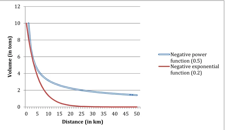
(15) Because of our aggregation of both jeans and sweaters into the commodity grouping ‘textile’ the flows of textile do not make sense from a logical (optimal cost) point of view. However in a gravity model these kinds of flows are allowed and modelled, as we will show in the next section. □ As mentioned in the Introduction and shown in Example 1 other factors besides distance like impurity (later represented by the level of homogeneity) are expected to influence the level of resistance too. One way to improve the current mapping and prediction of future commodity freight flows could be by developing a better understanding of the factors influencing the level of resistance. But before we concentrate on the factors influencing the resistance we will first discuss the resistance itself in more detail. Decay functions The level of resistance is represented by a certain metric (distance, time or general costs) in combination with a decay function. This function represents the decay in volume (tons) transported over increasing distance, time or cost. In gravity modelling the decay function often has the form of a negative power function (dij-β) or a negative exponential function (exp (-β*dij)). In these functions dij represents the resistance variable (for example distance) from supply to demand point. Parameter β is known as the decay parameter and determines the slope of the decay function. The graph below demonstrates an example for both decay functions. 12. Volume (in tons). 10 8 Negative power function (0.5) Negative exponential function (0.2). 6 4 2 0 0. 5. 10 15 20 25 30 35 40 45 50 Distance (in km). Figure 1.1: Example of negative power function and negative exponential function. The decay function (including the value of the decay parameter is normally estimated from sample data (actual freight flows). The source of the data can be a census, a procedure of systematically acquiring and recording information about a certain group of truck drivers, a logistical survey, a one-time survey under companies that have trucks for transport on road, or a statistical bureau, a governmental institution that gathers all types of data. The estimation of the decay function is generally an iterative process based on the volumes transported and related distances between the supply and demand points. An alternative procedure is based on the mean trip length (MTL) of a commodity 3.

(16) grouping (average weighted distance of all shipments) and the distances between the supply and demand points. However both procedures depend on actual freight flow data and these are not available at the moment in South Africa as no census or survey has been carried out recently. The statistical bureau does not has these data available either, as companies in South Africa are not obliged to hand over information about their freight flows. The current decay functions are therefore based on a (sophisticated) trial-and-error method that partly rely on decay functions from rail transport, actual flow figures from road transport and knowledge of industry experts. These figures are verified by common sense and feedback from practice. Based on these decay functions the flows are modelled and forecasts are made. To obtain national wide data for all industries in South Africa necessary for deriving accurate decay functions extensive logistical surveys, census or a new law (obligation to hand over freight flow information) are essential. However both surveys and census are expensive and highly time consuming and the implementation of such a new law is unlikely (because of serious confidentiality issues). Therefore obtaining the necessary data is almost impossible without governmental support or a financial sponsor. Flowmap Since the introduction of the national freight flow model a specific software package, Flowmap, is used to support the modelling of the flows. The software was designed by the University of Utrecht, the Netherlands, in 1990. It uses supply and demand tables (amount of supply/demand in each point), distance tables (from supply to demand points) and the decay functions as input to generate flows from supply to demand points. The flows are generated in such a way that these flows match the given decay function. This procedure is demonstrated in the example below.. Example 2. Flow modelling in Flowmap As mentioned before Flowmap uses the supply (in the origins, Oi) and demand (in the destinations, Dj) (Figure 1.2a), distance from the origin to the destination (Figure 1.2b) and the decay function (including the decay parameter) (Figure 1.2c) as input for the flow modelling. y = exp (-0.5*x). (a). (b). (c). Figure 1.2: (a) OD – graph; (b) Distance table; and (c) Decay function. In Figure 1.2a the origins (Oi) and destinations (Dj) and their amount of supply/demand (between brackets) is shown. A complete list of distances from every possible origin to every possible destination is given in the distance table (see simplified example in Figure 1.2b). The graph in Figure 1.2c shows how far the tons of goods are supposed to. 4.

(17) be transported. In this case a lot of tons will only be transported over a short distance while just a few tons will be transported over a long distance. Flowmap will now generate flows from the origins to the destinations. Many different configurations (so-called sets of flows) are possible. Next the different sets of flows (like for example the set presented in Figure 1.3a) are compared with the given decay function (in this case exp (-0.5*dij)). In Figure 1.3a we can see for example that 7 tons are transported from O1 to D1 and a 3 tons from O1 to D2. The remaining 5 tons of demand in D2 are supplied from O2. The comparison between the set of flows and the decay function is visually represented by Figure 1.3b. Finally the set of flows is chosen that fits best (in terms of distance and tonnage) with the given decay function.. (a). (b). Figure 1.3: (a) OD – flows; and (b) Flows matched with decay function. The best-fitting procedure within Flowmap is based on a comparison of the MTL from the set of OD-flows and the MTL of the applied decay function (in the range of the shortest and longest OD-distance in the set of OD-flows, see figure 1.3b). An example of this comparison can be found below (Equation 1.1 and 1.2). In Equation 1.1 Tij represents the total amount (volume) of flows from Oi to Dj (explained in detail in Section 2.2). Cij represents the resistance variable, in this case the distance from Oi to Dj, in both equations. In both equations we multiply the volume with the distance over which it is transported, sum over all these values and divide this sum by the sum of the total volume transported. MTL of OD-flows: (1.1) (Σi Σj (Tij * Cij)) / (Σi Σj Tij) = (13*1 + 8*2 + 5*3 + 4*4)/30 = 2 MTL of applied decay function (exp (-0.5*dij)): (1.2) (Σi Σj (exp(-β*Cij) * Cij ))) / (Σi Σj (exp(-β*Cij))) = (exp(-0.5*1) * 1)+(exp(-0.5*2) * 2)+(exp(-0.5*3) * 3)+(exp(-0.5*4) * 4)/ (exp(-0.5*1)+exp(-0.5*2)+exp(-0.5*3)+exp(-0.5*4)) = 1.92. In this case Flowmap compares the outcomes of the two equations (2 and 1.96). If no other generated set of OD-flows produces a MTL closer to 1.92 the flow presented in Figure 1.3a (with a MTL of 2) will be chosen. □. 5.

(18) If the decay parameter is unknown Flowmap gives the possibility to use an iterative procedure to derive the parameter based on the MTL of actual observed flows. In case no applicable decay parameter is available from earlier research and there is a lack of actual observed flows (so no reliable MTL can be derived), as is the case in South Africa, an alternative way to obtain a decay parameter needs to be created. The overall aim of CSCM is to improve the model every yearly cycle both in functionality as well as accuracy of the current and forecasted flows. As the decay function is one of the main input variables for the flow modelling improving, this function would improve the accuracy of the currently mapped and forecasted flows. 1.3 Problem statement As mentioned earlier the idea within CSCM is that the decay function is influenced by more than just the distance between supply and demand points. The expectation is that a better insight in the factors influencing the decay will improve the accuracy of the decay function and therefore the mapped and forecasted freight flows. This leads to the central research question.. Central research question How can the current decay functions of the commodity freight flow model applied on the freight flows of South Africa transported by road be improved in a way that both the current mapping of the freight flows as well as the forecasts of the freight flows will be improved by focussing on better insights in the factors influencing decay? To answer every aspect of the central research question in a structured way a set of sub research questions are formulated. Combining the outcomes of these sub studies should be sufficient to come to a conclusion regarding the central research question at hand. Sub research questions 1. How is the commodity freight flow model for South Africa built up? (Which modelling techniques form the backbone of the model and why? What changes have been applied since the introduction of the model? What is the status quo of the model?) To be able to speak a common language with the designers and current users of the commodity freight flow model it is important to understand how the model was initially established, which modelling techniques have been applied and what changes the model has gone through. This brings us to the current status of the model. Being aware of the status quo makes it possible to indicate the improvement opportunities of the research on decay functions. Moreover it forms the basis for later validation of the suggested improvements. 2. Which decay functions are currently used in the commodity freight flow model and why? (What decay function and parameters are applied and why? How are they derived? What is the influence on the model?). To make suggestions for improvement understanding the role of the decay functions in the commodity freight flow model is essential.. 6.

(19) 3. What decay functions are available/commonly used in scientific research? (What decay function and parameters are applied in comparable models/modelling techniques and why? How are they derived?). To be able to question the currently used decay functions it is important to know what other functions are available to describe decay and to know their advantages and limitations. 4. What factors that could influence the decay in freight transportation are known in literature? (Which are currently applied or have been applied in the past in commodity freight flow models and why? What is the influence on the model?). The decay function is currently established based on a trial-and-error method without a proper scientific background. To be able to construct the decay function in an academically appropriate way based on the factors by which it is influenced, these factors obviously need to be known. 5. How can the present commodity freight flow model be improved by including insights on the factors influencing the decay?. After our analysis we expect to know how the different factors influence decay and to which extent. These insights should eventually make it possible to establish a regression model that enables CSCM to derive decay functions without performing a nation-wide logistical survey or census or waiting for the implementation of the obligation for companies to hand over their freight flow data. This scientific method should eventually lead to better founded forecasts for the future. 6. What data are required for the model improvement and how can it be acquired?. Part of the analyses will be the measurement of the influencing factors and the scoring of the commodity grouping against these factors. This will be the biggest share of data needed and needs to come from external parties. Next to that current flows (output from the model) are needed to test the results of the decay function improvements, data that come from CSCM itself. 7. How should the improvement of the decay functions be measured and validated?. Although both the decay functions currently used and the output flows from the model are not proven to be totally correct they are the best values currently available. The validation will be done based on (parts of) the flows that are most reliable. 8. How should the improved model be used and maintained?. The improvement will be limited to the decay functions so the changes to the structure of the model are expected to be rather small. The whole model is based on Flowmap. This program will have limitations concerning input variables. That fact will be taken into account throughout the research. The overall perception is that the basic way the model is currently used will not change majorly.. 7.

(20) The biggest challenge will be to obtain the necessary input data to score the influencing factors as these scores are likely to change over time. This counts both for the yearly update as well as for the future forecasts. 1.4 Research purpose In the introduction of this report the main purpose of this research, increasing the accuracy of the model output (currently mapped and predicted freight flows) by improving the current decay functions, has already been mentioned. By gathering more knowledge about the factors influencing the decay of transported volume over distance establishing the decay function will become more fact based. Therefore the accuracy of both currently mapped flows and predicted flows is expected to increase. In the current situation the decay function is static for all the predicted years as no indicators for change are available. However Iacono et al. (2008) already indicated that the decay function is often studied over time because of its characteristic of being dynamic and changing in response to transportation network development for example. So by knowing the factors influencing the decay it should be possible to predict changes in the decay function if a change in one or more influencing factors is expected. Therefore a significant increase in accuracy is expected in the predicted flows.. The shift from the current (sophisticated) trial-and-error method towards a more fact based approach to establish decay functions makes it possible to give a validated explanation for the chosen decay function, a requirement of the current clients of CSCM. An important additional advantage of the fact-based approach is the time consumption of the process. The model has to be rerun for every adjustment of the decay function, which takes a lot of time, especially if it has to be done for 64 commodity groupings individually. The current approach uses trial-and-error, which means a lot of adjustments. The fact-based approach should be able to reduce the amount of necessary adjustments drastically and therefore the time needed for rerunning the model. 1.5 Research method The first steps to understand the composition, role and behaviour of decay functions within gravity modelling and the commodity freight flow model in specific are conducting a literature study and interviewing the people involved in the design of the model, the construction of Flowmap and people working with gravity modelling on a regular basis (the experts). The knowledge about the basics of decay functions forms the basis for the analysis of factors influencing the decay. Again literature and interviews will form the starting point, resulting in a list with possible influencing factors. Based on statistical methods the real influence of and correlation between the influencing factors should become clear. This should generate sufficient input for the final formula replacing the old decay function. To be able to carry out statistical analyses sufficient and verified data need to be available. Therefore currently available data need to be verified and in-depth research should be done on the characteristics and current flow behaviour of the different commodity groups. Understanding their characteristics and current flow behaviour are essential to be able to make realistic comparisons among them during workshops with. 8.

(21) the CSCM team. Therefore different data sources and knowledgeable people will be consulted. 1.6 Boundaries The research only concerns the transportation of goods on road The commodity freight flow model combines the flows of goods (no passengers are included) from all the different available modes in South Africa. However this research only concerns the transportation of goods on road as the flows of goods on the other modes are known based on detailed and reliable data. Road however counts for about 90% of the total tonnage of freight transported and is therefore of high interest for CSCM and her clients.. The deep dive analysis will be limited to a maximum of 10 commodity groups The deep dive analysis will be limited to a maximum of 10 commodity groups that are expected to cover the upper and lower bounds of the rating spectrum for every influencing factor. This will speed up the process of discussing and verifying figures (rates) during the workshops, limit the amount of time needed for this phase and is expected to deliver sufficient information for the next steps in the research. The other commodity groups will be rated and verified outside of the workshops based on comparisons with the in-depth researched commodity groupings and the derived upper and lower bounds, without carrying out in-depth research on them. Verification will be based on the latest modelled flows Verification will be based on the latest modelled flows. These flows are no exact replication of the actual flows but they currently give the best indication. The lack of actual flows is a problem experienced often in this field of research as mentioned by De Jong et al. (2004) and Bröcker et al. (2010). In these cases different sources of data have to be combined to establish the overall view. One of the factors influencing the accuracy of the output of freight flow models is the large amount of modifications necessary to make the already scarce, available data suitable as input for the model (De Jong, 2004). Although the modifications may have a serious impact on the output of the model this impact will be the same for both the currently modelled flows as for the flows established based on the model improvements. Therefore the modification issues are not taken into account within this research. Manoeuvring within the possibilities and boundaries of Flowmap The commodity freight flow model is based on and built up around Flowmap and its required input variables. Changing the software package (switching to another provider than Flowmap) is far from likely as it will be very costly and time consuming. Another possibility would be to change the structure/code of Flowmap. However this will also be a costly and time-consuming exercise, as CSCM does not have the authority nor the necessary knowledge to make changes in the program structure by herself. Therefore the intention of this research is to manoeuvre within the boundaries of what is possible within the structure of Flowmap. 1.7 Thesis structure The remainder of the report is organized as follows. Chapter 2 consists of a literature review where the focus will be on gravity modelling, estimating decay functions, the factors influencing decay and topics from closely related study fields. An in-depth. 9.

(22) overview of the commodity freight flow model is given in Chapter 3. The analysis methodology is presented in Chapter 4. Chapter 5 describes the data used to perform the proposed analyses. The results of the study are presented in Chapter 6. Chapter 7 is used to discuss the results of the study and Chapter 8 concludes the report with most important findings, an answer to the research question and recommendations for further research. On the next page a schematic overview of the structure is shown.. 10.

(23) 11.

(24) 2. Literature review We will use this chapter to review the history and current application of gravity modelling (Section 2.1). The resistance variables and decay functions as well as the way they are estimated from sample data will be discussed (Section 2.2). We will review the factors known in literature that have been proven to influence the decay functions in freight transportation (Section 2.3) and we present and evaluate decay functions used in comparable models (Section 2.4). We will conclude this chapter by touching on some freight flow related topics (Section 2.5). In the last decades the decay function has gain a lot of attention in scientific research. Numerous studies especially in travel behaviour of pedestrians (willingness to travel for work for example) and cross border freight transport have been conducted in the last decades, aiming to define and derive the “correct” decay function (Haynes, 1984). However the decay function that should explain the freight flows within country borders seems to be of less interest. The studies that are dedicated to national freight flows only slightly touch the decay function but there seems to be a lack of research questioning distance to be the only factor influencing the decay. The lack of research on factors influencing the decay in transport freight flows may be partly explained by fact that the field of scientific research on this topic is rather small and the required budget to conduct proper studies in this field is high. Besides that the level of detail and the accuracy of the data available in most other countries with a freight flow model in place are higher than the detail and accuracy of the South African data. Therefore the derived decay functions are more accurate and the need for more information on the influencing factors is lacking (no regression model needed). The amount of commonly available publications about decay functions within national freight flow models may be limited (Östlund, 2003 and Hensher, 2008) but as said earlier much about decay functions and their role in transportation modelling in general has been researched. We will now first introduce gravity modelling before we focus on decay functions and the factors influencing them. 2.1 Gravity modelling The universal gravitation law Although a theoretical explanation for the application of the empirical gravity equation for commodities was only given in 1979 (by Anderson) the gravity equation was by then already intensively used as a trade device for over a quarter of a century. The principle of the gravity equation, originally derived from the universal gravitation law in physics founded by Newton (in 1687), describes the interaction (force) between two points (masses) based on the size of both points and the distance between them (Roy and Thill, 2004). The level of interaction is proportional to the product of the two masses and inversely proportional to the squared distance between them. The original expression has therefore the following form:. (2.1) F = G*(m1*m2/r2) Here F is the force between the masses, m1 and m2 are the first and second mass and r is the distance between the masses. G is the gravitational constant, a constant of proportionality used to make sure that F has a meaningful magnitude.. 12.

(25) The gravity models currently used in the field of transportation are all based on this early gravitation law. As expected these models have for various reasons evolved over time, some just slightly others, like the traffic-demand equations, have started to take on the characteristics of large multiple regression models (explained in Section 4.7) (Taaffe, 1996). Later in this section we will show some of the evolvements in the model expression like the masses that may often be replaced by supply and demand and the squared distance that may be replaced by a combination of a resistance variable and a decay function. Before the model formulation is discussed in more detail it is necessary to see where the gravity model fits in the broader process of transportation forecasting to understand the model components involved. An easily understood model that is often used for transportation forecasting purposes is the four-step model. The model includes all basic steps involved in the forecasting procedure. We will discuss the model and the separate steps below. The four-step model The four-step model (FSM) was designed and applied the first time during the early 1950s. It was initially meant for the modelling of travel behaviour to evaluate trafficengineering improvements. Later it has been used for urban transportation planning, environmental concerns and multimodal (multiple modes of transport) planning (McNally, 2000). Since the late 1970s when was recognised that the initial model was not suitable for the emerging policy concerns many model upgrades and improvements have been conducted. This has led to the start of what has grown to become the activitybased approach and base for the current modelling of passenger transport. Although the four-step model was, like many other model concepts, created for travel behaviour of passengers initially freight transportation adopted this model too. It has been in place for many years now. Each step had to be adapted to be applicable for freight transportation forecasting but the basic principles have stayed the same (De Jong, 2004):. *. Trip generation (supply and demand): the quantities (in tons) of goods to be transported from the various origin zones and the quantities to be transported to the various destinations zones are determined. They form the marginals of the OD-matrices (see Figure 3.3 for an example of an OD-matrix and Sections 3.2.2 and 3.2.3 for more explanation).. *. Trip distribution: the flows of goods transported from points of origin to points of destinations are determined, often using a gravity model function. They form the cells of the OD-matrices.. *. Mode choice: the allocation of the commodity flows to modes (e.g. road, rail) is determined. This modal model may be of the logit form (statistical model for predicting human choice behaviour), developed by McFadden.. *. Route choice: after converting the flows in tons to vehicle-units, they can be assigned to networks.. Although the steps above seem to have a fixed sequence the possibility of feedback is allowed and therefore makes the model principles better aligned with other existing. 13.

(26) concepts (like supply-demand equilibrium). A drawback of the model is that it has difficulties in capturing adequately the factors that influence shippers and carriers route choice behaviour (Southworth, 2006). Institutional and decision-making structures are simply lacking in current applied models of this kind. These components, appearing in other models, seem to play a significant role in the explanation and forecasting of the flows. However to be able to use these kinds of functionalities certain input data are essential. If these data components are not available the four-step model does not have serious limitations for the user compared to the other models (that obviously need the data to be able to make their extra features usable). Recent model expressions As mentioned above the gravity model is commonly used in the second step of the fourstep model, the trip distribution. However the general model expression for this step differs from the original expression of Newton. The sizes of the supply and demand points are expressed in the level or volume of supply (Oi) and level or volume of demand (Dj). The squared distance between the points has been replaced by a more general resistance variable (Cij) combined with a certain decay function. Cij can still represent the distance between the origins and destinations but also the travel time between these points or general (transportation) costs. The decay function (in this case a negative power function) describes the decay in tons transported versus an increasing resistance variable. Parameter (β), the decay parameter, determines the slope of the decay function. The expression may therefore have the following form:. (2.2) Tij = α *Oi*Dj*Cij-β In this expression Tij is the amount of trips from Oi to Dj and therefore comparable with the force of interaction (F) in the original model expression of Newton. α is the substitute for the gravitation constant (G) having the same function in reducing the estimated flows to more realistic magnitudes (with α ≥ 0). The decay parameter (β) is generally positive. Only in case more volume gets distributed over long distance than over short distance (which is unlikely) the parameter becomes negative. The gravity model can also be used for a combination of the first and second step of the four-step model, the trip generation and the trip distribution. This model variant is used in case the actual supply and demand values of the different places of origin and destination are unknown (in African countries for example). The variables in the gravity model expression have to be changed again slightly. If we recall the original gravity model expression, size is expected to be the most important indicator for flow generation. The most commonly used indicator of size is the gross domestic product (GDP), in the new model expression represented by (Yi) for the origin and (Yj) for the destination. Next to GDP other origin and destination specific characteristics (like for example the size of the region of origin, size of population or productivity) can be included (Bröcker, 2010). The expression may have the following form: (2.3) Tij = αYi*Yj*Cij-β. 14.

(27) This model expression (in more sophisticated form) is often used in cross border freight flow modelling, as GDP is known for most countries with a reasonable level of accuracy. Many different variants of the original gravity model are currently in use within freight flow modelling and many other research fields. However the basic principles have not changed tremendously. We still see substitutes for the size of origin and destination in every model as well as combinations of resistance variables and decay functions. In the next section we will have a closer look at these last two elements. 2.2 Resistance variables and decay functions In the previous section both the resistance variable and the decay function have been mentioned. The combination of both is referred to as the level of resistance to transport freight from certain origins to certain destinations. The combination determines how far, long or against which costs certain goods are being transported. The role of the resistance variable and the decay function in gravity modelling is significant. A more detailed review is therefore desirable and given below. Resistance variables In the original model expression of Newton (Equation 2.1, see previous section) the amount of interaction between two masses was inversely proportional to the squared distance between the two masses. Distance can be seen as the resistance variable within this expression. Nowadays distance is still widely used as a resistance variable in gravity modelling however alternatives have been introduced. Instead of transportation distance, resistance can also be measured in transportation time or transportation costs (Iacono et al., 2008). Bröcker et al. (1990) even included geographical, historical and cultural transportation barriers in their resistance variable. The choice for the resistance variable used in the gravity model highly depends on the purpose of the model and the available data. In freight flow modelling distance is the most common resistance variable. The necessary data are often more reliable compared to transportation times as only origin, destination and (road) network are needed for the distance (objective data) compared to the travel times which are self-reported and therefore subject to the bounds of human perception and cognition (Iacono, 2008). Moreover from a cost calculation perspective (in case of non-perishable goods) distance is often the most important denominator. The use of travel time as resistance variable is far more popular in urban passenger transportation models, as travel time is the most important denominator for the far majority of the people travelling for example from home to work, school or the shopping mall. Distance related cost components like petrol and truck depreciation are by far the biggest cost components related to road freight transportation. From a macroeconomic perspective they can be assumed to behave more or less linear with distance. Because of this assumption of linearity the cost components can be represented by distance only and no general transportation cost variable is needed. Model simplicity motivates the preference of distance above a general transportation cost variable in case of road freight transportation. There are situations were certain significant costs cannot be linked to distance or travel time (for example an airplane charter) in these cases a transportation cost variable can be used. The transportation barriers mentioned by Bröcker et al. (1990) are specifically meant for. 15.

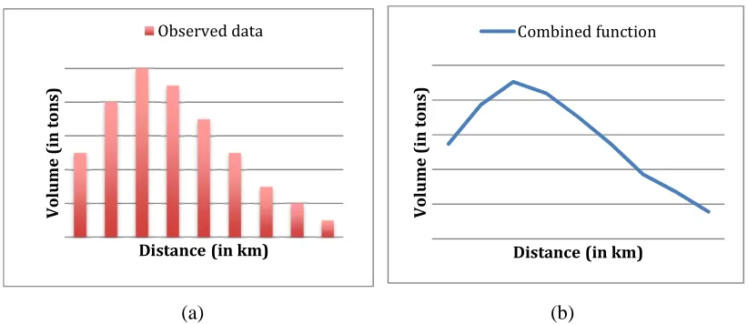
(28) gravity modelling in international trade. Next to the fact that different resistance variables can be used there are alternative ways to measure these individual variables. Distance can for example be based on a real road network, a penalized road network or the Euclidean distance among others. The choice how to measure distance depends on a range of variables but one of the important aspects is the mode of transport as the distance between origin and destination can differ a lot when travelling by airplane following Euclidean distance or by truck using the road network. Another aspect that influences the choice of measurement is the sub-goal of the model, does it aim for shortest distance, avoiding of rural roads, avoiding of congestion etc. While making these choices and model assumptions regarding the resistance variable it is essential to take the demand for data and the influence on the model complexity into account. The other component necessary to obtain the level of resistance in gravity modelling is the decay function. This component is reviewed below. Decay function In the model expression in the previous section (Equation 2.2) the decay function is a negative power function. However the function can also be specified as the inverse of the resistance variable or with the more common specification of a negative exponential function exp(-β*Cij). A combination of the functions is also possible. This so-called combined function, Cijγ*exp(-β*Cij), is often used when the observed data show a pattern comparable to the form of Figure 2.1 (Ortuzar & Willumsen, 2001). This kind of data is for example observed in vehicle transport in urban areas.. Observed data. Volume (in tons). Volume (in tons). Combined function. Distance (in km). Distance (in km). (a). (b). Figure 2.1: Combined function model fit. The type of decay function used in the gravity model depends on the data related to the subject of interaction (sample data). This can be a set of trip lengths of a transported commodity group for example. The decay function that has the best fit with the data, based on a goodness-of-fit test (see Section 4.6), will normally be used. However the choice for the decay function can also be limited by the software used for the modelling. 16.

(29) process. This is the case with Flowmap that only provides the choice between a negative power and a negative exponential function. Regardless of the mathematical expression used, the decay function is intended to convey the decline in interaction as the distance, time or cost between origin and destination increases. As mentioned earlier, the (steepness of the) slope of the decay function is determined by the decay parameter. We give a more detailed description of this parameter below. Decay parameter Simultaneously with the decay function the decay parameter is estimated from the sample data. In essence there are two primary methods (similar to other spatial interaction models) for estimating a decay function and parameter: linear regression using ordinary least squares on a transformed decay function and estimation of a nonlinear model using maximum likelihood estimation (MLE) techniques. To be able to use the ordinary least square method the model (for every type of decay function) needs to be transformed into a linear-in-parameters form by taking the natural logarithm of both sides (Fotheringham & O' Kelly, 1989):. (2.4) ln(Tij) = ln(α) + ln(Oi) + ln(Dj) - β*ln(Cij) The parameters in the model will be unbiased and consistent except for the estimate of α, produced as eln(α). This constant will be underestimated unless the model fit is perfect (Heien, 1968). Depending on the level of desired accuracy this deviation becomes more important. The parameters in the unconstrained gravity model can also be estimated via a maximum likelihood technique if it is assumed that interactions are the outcome of a Poisson process (Flowerdew & Aitkin, 1982). Several algorithms for the estimation of the maximum likelihood are available for example the Newton-Raphson procedure (Jennerich, 1976). These are the two commonly used techniques for estimating decay parameters in case sample data are available from surveys, census or a statistical bureau. The alternative method based on the MTL (see Section 1.2) is less accurate and therefore less frequently used. In case the sample data are not available, as is the current case in South Africa, we have to look for an alternative, as mentioned in the first chapter. Obviously, as also mentioned in that chapter, CSCM has an alternative way to derive the current decay functions but this method was designed from a practical perspective and lacks academic background. The proposed alternative to this method assumes other factors besides distance to influence decay. Therefore in the next section we will present the findings about these factors from literature. 2.3 Factors influencing decay Repeated applications to real-world transportation situations have made it clear that there is no single “correct” decay exponent (decay parameter) for all situations that reflect some underlying law of human spatial interaction (Taaffe, 1996). Variations in the decay function itself have become the subject of empirical study since it became apparent that decay parameter (β) values will be different for different years, different modes, different commodities transported, to name a few.. 17.

(30) Several studies have pointed out evidence for the relation between the value of goods and the decay parameter. It is stated that higher-value goods should be less sensitive to the increased costs of long-haul commodity shipment since transport cost form a smaller part of manufacturer’s total costs (Taaffe, 1996). Therefore higher-value goods are associated with lower value decay parameters. Another negative correlation that is empirically studied is the one between regional specialization in the production of a good and the value of the decay parameter (Black, 1972). In case a region (for example the south-east of South-Africa) is highly specialised in the production of a particular good (for example avocados), it is less likely to be sensitive to distance in its shipments as the avocados have to be transported to the west coast market anyway. A commodity grouping such as stone that is widely available will be dominated by short-haul shipments because of the proximity of competitors and will therefore end up having a high value for its decay parameter. The regional specialization should be seen relative to the other regions examined. So regional specialization is high when there is only one or a few regions able to produce a certain good. Alternatively, if the entire production of the good is consumed locally due to economies of scale, perishability, and so forth, the decay parameter will be high (Black, 1972). Black also investigated the relation between decay and the value (per unit weight) of goods, however he concluded that regional specialization had a higher reducing effect on the value of the decay parameter than the high-value per unit weight. Based on the relationships Black had found he tested a multiple regression model to estimate the decay parameter. He included two variables; “regional specialization” (supply side) measured by the proportion of total flows shipped from the largest shipping region and “local consumption” proportion of total flows that are produced and consumed in the same region. This multiple regression (with correlation coefficients for regional specialization of -0.453 and for local consumption of 0.854; both significantly different from zero at the 0.01 level) accounted for approximately 87 percent of the variation in the decay parameters examined. This method is in line with the alternative approach suggested at the end of the previous section. However for Black the usage of this approach was not motivated by a lack of access to actual flow data, which were available, but was meant as a study to investigate the feasibility and accuracy of this alternative. As he had actual flow data available, he was able to compare the freight flow model output based on the decay parameters estimated by the regression analysis with the freight flow model output based on the decay parameters estimated. For this estimation he used an iterative process based on the actual flow data. Generally, the accuracy of both estimated decay parameters turned out to be nearly similar. A relationship between the value of the decay parameter and a macroeconomic phenomenon is obviously also possible. For example an increase in the price of petrol will make long-haul shipments less attractive and will therefore result in a stronger decay on the distance goods are transported. Increasing petrol prices will influence the decay parameter of all commodity groupings (as it is a macroeconomic phenomenon). However the relative impact will be less for higher-value goods and is therefore in line with reasoning that higher-value goods have lower decay parameters. Although the studies mentioned above indicated a great diversity in the used values for the decay function, some scientists have suggested averages. For the decay (negative power function) on road a value of 2.0 has been suggested for the decay parameter based. 18.

No results found