Design of control strategies for UAVs physically interacting with each other and the environment

University of Twente

EEMCS / Electrical Engineering

Robotics

and

Mechatronics

Design of control strategies for

UAVs physically interacting with

each other and the environment

R.T.L.M. (Ramon) Tummers

MSc Report

Committee:

Prof.dr.ir. S. Stramigioli Dr. R. Carloni Mr. M. Fumagalli, PhD Dr.ir. R.G.K.M. Aarts

Contents

General introduction

3

Research article

5

Conclusions

17

Appendices

19

A Gripper design

19

B Ducted fan manual

25

General introduction

The field of autonomous aerial service robots increased significantly in the

last couple of years. The main motivation behind this is the growing wish

to be able to do tasks at hard to reach places, e.g. skyscrapers and

wind-mills. Here labour costs can be reduced significanly when aerial vehicles are

used in stead of regular personnel as they need expensive machinery and/or

scaffolding to reach these places.

When these unmanned aerial vehicles (UAVs) will be used in real

ap-plication scenarios like the ones mentioned above, the ability to interact

actively and safely with the environment is required. Also interaction

be-tween several UAVs is of importance as some tasks might by impossible to

conduct with only one UAV. All this interaction takes place in free-flight,

so without constraints to the ground.

The main goal of the research presented in this report is to design a

con-trol architecture that complies with these requirements. This design will be

done through simulation and experimental validation of a quadrotor UAV

endowed with an edge mounted robotic arm and a gripper, which in total

make the flying hand, and make it grasp either a static or a moving

ob-ject. The main focus will be on verifying proper working of the controller

throughout different system states: free-flight, docked to either a static

ob-ject connected to a vertical wall or a dynamic one and fly away with an

object. Lastly path tracking in the dynamic docked state will be verified

which will require some added high level control of the system.

The stability of the control architecture is achieved by considering

stan-dard passivity-based feedback design techniques, where the stability of a

desired equilibrium point is obtained by shaping the energy function of the

system to have a desired minimum (

energy-shaping

), and then by

dissipat-ing energy to asymptotically converge to it (

damping-injection

). It will be

shown that the complete system can be described by a cascade of these

systems.

The main part of the research, i.e. the system analysis and control

design, is presented as an article. Afterwards some conclusions will be drawn

and recommendations given.

For the actual construction of the total aerial manipulation system a

gripper that can be added to the robotic arm is required. The design hereof

was done by reviewing several concepts by means of modelling. Afterwards

one design is chosen and build. A full review of this process can be found

in Appendix A.

The idea of attaching the object to another UAV was desired at first.

Therefore the Ducted Fan UAV, designed by the University of Bologna was

chosen. Its hardware and software needed to use the apparatus have been

reviewed for this project and can be found in Appendix B. Unfortunately

during the research the system was deemed not usefull at this stage for

this research due to the non-robustness of the system. For future reference

however it is still included as an appendix to this report.

Modelling and Control of an Aerial Manipulation System with a

Compliant Gripper

R.T.L.M. Tummers, M. Fumagalli and R. Carloni

Abstract— In this research, we present the design, simulation and experimental validation of a control architecture for an aerial manipulation system, i.e. a flying hand, that consits of an unmanned aerial vehicle, a robotic arm and a compliant gripper. The flying hand can realise mobile manipulation by grasping an object fixed to a vertical wall or a moving object that can exert dynamical forces. The goal of this work is to show that the overall control architecture allows the flying hand to approach the wall or the moving object, to dock on the object by means of the gripper and either detach the object from the wall or realise grasping and tracking of the mobile object in case of mobile manipulation. The control strategy has been implemented and validated in the simulated model as well as in experiments on the complete aerial manipulation system.

I. INTRODUCTION

In recent years, the research interest in aerial service robots is increasing. One of the main goals is to use unmanned aerial vehicles (UAVs) in real application scenarios to support human beings in all those activities that require the ability to interact actively and safely with the environment not constrained to the ground, but indeed airborne [1]. Also interaction between UAVs plays a role as some tasks might require more than one UAV to accomplish them, e.g. carrying large and heavy objects.

Several works attest the interest in such challenging con-trol scenarios. For instance, grasping and transportation using a fleet of quadrotors is considered in [2], and extended in [3] to assemble an infrastructure. The design of control architectures for the aerial manipulation of large objects using cables is considered in [4] and extended in [5]. In [6], a quadrotor helicopter is employed to clean a surface while hovering, where an additional propeller is employed to counteract contact forces while maintaining the stability of the vehicle. In [7], the physical interaction between a ducted fan aerial vehicle and the environment is considered. The approach considers to switch the control law in order to take into account for possible constraints deriving from the presence of contacts. Aerial grasping using an autonomous helicopter endowed with a manipulator is considered in [8] and [9]. In these cases, the analysis focuses on the stability of the vehicle during the interaction with a compliant environment. A prototype of miniature aerial manipulator has been proposed in [10].

This work has been funded by the European Commission’s Seventh Framework Programme as part of the project AIRobots under grant no. 248669.

[email protected],{m.fumagalli,r.carloni}@utwente.nl, CTIT Institute, Department of Electrical Engineering, University of Twente, The Netherlands.

In this paper, we present the design, simulation and experimental validation of a control architecture for a flying hand and mobile manipulation with a moving object. The flying hand is composed of three different parts: a quadrotor UAV, a robotic arm and a gripper. The latter two combined is the robotic manipulator. The goal of the controller hereof is to show that the system can have three different operating states: free flight, docking on the object attached to a vertical surface, fly away with the object. In case of mobile manipu-lation the latter will be moving and exerting dynamical forces as well as impose a trajectory on the quadrotor UAV.

The stability of the control architecture is achieved by considering standard passivity-based feedback design tech-niques, where the stability of a desired equilibrium point is obtained by shaping the energy function of the system to have a desired minimum (energy-shaping), and then by dissipating energy to asymptotically converge to it (damping-injection).

The paper is organised as follows. In Section II, the overall mobile manipulation system is presented together with its dynamic model. In Section III, we propose the control strategy, which is validated in both simulations, in Section IV, and experimental tests, in Section V. Finally, concluding remarks are drawn in Section VI.

II. SYSTEM DYNAMICS

In order to design the control laws and analyse the stability of the flying hand while grasping an object, both fixed and in mobile manipulation, the overall model of the system dynamics is required. First, we discuss the structure of the complete system, secondly, each part is modelled individually.

A. System Overview

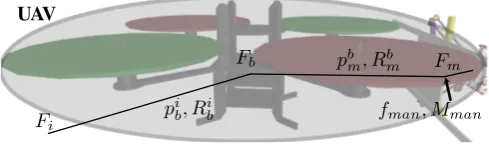
The complete gripper system is composed of three parts. The first is the underactuated quadrotor UAV, i.e. an AscTec Pelican quadrotor [11], as shown in Figure 1.

fman, Mman

Fb F_m

Fi p

i b, Rbi

pb m, Rbm

UAV

Fig. 1. The quadrotor UAV and its reference frames.

a base plate, with three actuators and three legs (composed of a thigh and a shin parallelogram). It enables Cartesian movement in the workspace of its end-effector and can be used to track a certain point in the inertial frame regardless of the movements of the base plate, which is rigidly attached to the UAV.

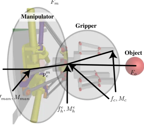
Finally, the third part is an underactuated gripper, whose design is based on the work presented in [13]. The mechan-ical structure of the gripper consists of three fingers, with two phalanges each, and is actuated by one single motor. The construction of the gripper is such that form closure is guaranteed. The sketch of the robotic arm, the gripper and a fixed object is shown in Figure 2.

fe h, Mhe

Fe

pm

e Fo

Ffi

Fm

fc, Mc

fman, Mman

Object Manipulator

Gripper

Fig. 2. The robotic manipulator, the gripper, the object and their reference frames.

For the case of mobile manipulation the object takes the form of a rod, to which the manipulator system can dock, connected to a wand that can exert forces on the system as well as impose a position.

B. Notation

Before proceeding with the description of the system dynamics, all used symbols are briefly explained for clarity. With reference to Figure 1 and Figure 2, the kinematic notation is:

• Fi,Fb,Fm,Fe,Ffi andFo, the inertial frame, the body frame of the quadrotor UAV fixed at its centre of gravity (c.g.), the base frame of the robotic arm, the base frame of the palm of the gripper (coincident with the base frame of the end effector of the robotic arm), the frame at the contact points on the fingers of the gripper and the object frame;

• pi_b = [xi_b, y_bi, z_bi]T and R_bi ∈ R3×3 the position and rotation matrix of the quadrocopter’s c.g. with respect to the inertial frame,Fi;

• pbm= [xbm, ymb, zmb]T andRbm∈R3×3 the position and

rotation matrix of the robotic arm’s base with respect to the frame at the quadrocopter’s c.g., Fb;

• pme = [xme , yme , zem]T andRme ∈R3×3 the position and

rotation matrix of the palm of the gripper with respect to the robotic arm’s base frame,Fm;

• peo = [xeo, yoe, zoe]T and Reo ∈ R3×3 the position and

rotation matrix of the object with respect to the palm of the gripper;

• po_fi = [xo_fi, yo_fi, zo_fi]T andRo_fi ∈R3×3 the position and rotation matrix of each of the contact points i of the gripper’s fingers with respect to the object frame,Fo;

The dynamic notation is:

• g the gravitational acceleration;

• muav, Juav are the quadrotor UAV’s mass and inertia matrix;

• fpb∈R3 the total thrust on the quadrocopter generated

by its propellers, fm

man ∈R3 the force the robotic arm and the UAV exert on each other at the robotic arm’s base;

• Mgyb ∈ R3 the moment vector due to the gyration effects of the propellers of the quadrocopter, Mb

p =

[Mx, My, Mz]T ∈R3 the control torque of the vehicle,

Mm

man∈R3 the reaction torque the robotic arm and the UAV exchange at the robotic arm’s base;

• fImm, M

m Im∈R

3 _{the vectors of all the dynamical forces}

and moments due to the absolute motion of the robotic arm inFm;

• f_Ie_h, M_Ie_h ∈R3 the vectors of all the dynamical forces and moments due to the absolute motion of the compli-ant gripper inFe;

• f_he, M_he∈R3 the force and moment vectors the gripper and the robotic arm’s end-effector exert on each other; • f_objo , M_objo ∈ R3 the force and moment vectors that make up the total wrench, wobj, the object exerts on the gripper’s fingers and palm in the object frame,Fo;

• fpb = [xbp, ypb, zpb]T ∈R3 the total thrust on the ducted

fan generated by its propeller and vanes;

• Mgyd ∈ R3 the moment vector due to the gyration effects of the propeller of the ducted fan, Md

p =

[Mx, My, Mz]T ∈R3 the control torque of the vehicle.

From a dynamical point of view, the complete system is seen as a cascade of subsystems, interconnected at certain points by means of localised interaction forces and moments. It is assumed that the system interacts with the environment (i.e. a static object or a mobile one) by means of the gripper’s base and the phalanges only, i.e. only in Fe and

Ff. Furthermore, the connections between the UAV and the

robotic arm’s base inFmas well as between the robotic arm’s

end-effector and the gripper’s palm inFeare assumed to be

rigid. The quadcopter UAV itselve inFbis unconstrained and

can thus move freely with respect to the inertial frame,Fi.

C. The Quadrotor Dynamics

The quadrotor is an underactuated system, since it has only four control inputs fi, i.e. its propellers, and six degrees

between the generated force of each propeller and the total thrust and torque exerted on the quadrotor UAV’s c.g. is given by     fb p Mx My Mz    =    

1 1 1 1

0 ₋d 0 d

d 0 ₋d 0

−c c ₋c c

        f1 f2 f3 f4     (1)

where d is the distance between the quadrotor UAV’s c.g. and the centre of the propeller, and c is the ratio between the propeller reaction torque and generated thrust. Using this, the full dynamics of the quadrotor UAV can be described by

muavv˙i_=muavgzˆi_+fb

pRib[0,0,−1]T +RibRbmfmanm Juavω˙b,i_b =₋ωb,i_{b ×}Juavωb,i_b +Mgy+Mpb

+Rmb Mmanm +Rbmfmanm ×pbm (2)

whereω˙b,i_b andω_bb,i are the rotational velocity and acceler-ation of the quadrotor UAV with respect to Fi expressed in

Fb, respectively; v˙i the linear acceleration of the quadrotor

UAV’s c.g. in Fi.

D. The Robotic Arm Dynamics

The dynamics of the robotic arm can be compactly described by dividing them into the internal and external dynamics. The former includes inertial and gravitational con-tributions as well as the dynamic influence of the actuators. The latter upholds forces and moments exchanged at the end effector with the gripper and due to interaction with the environment. From the equilibrium of forces and moments the dynamics of the robotic arm inFmare described by:

fm

man=fImm+R

m e fhe

Mmanm =MImm+R

m

e Mhe+Rme fhe×pme (3)

E. The Gripper Dynamics

The dynamics of the gripper are similar to the dynamics of the robotic arm. The dynamic contributions can be divided into internal and external, i.e. the gripper is attached at the robotic arm’s end-effector and is the source of all forces and moments exchanged here. Also the gripper can be loaded by an external force, given by the interaction with the object. Therefore, the dynamics of the gripper can be described by

fhe=fIeh+R

e ofobjo Mhe=MIeh+R

e

oMobjo +Reofobjo ×peo (4)

F. The Environment

The system is allowed to be in three different states: free-flight (no object), docking (on the object) and aerial grasp (with object). Therefore, both fo

obj and Mobjo in Equation 4 can have three different interpretations, depending on which state the system is in. These three states and their influence on the system are explained hereafter.

1) Free-flight state (no object): In this state, the UAV is in free flight and no object is grasped. This results in no external force and moment, i.e.,

fobjo = 0 Mo

obj= 0 (5)

2) Docking state (on the object): In this state, the quadro-tor UAV is docked on the object and, more precisely, it is docked by means of the gripper that is grasping the object attached to a vertical surface. The reaction forces and moments are partly due to the contact between the object and the base of gripper and partly due to the interaction between the object and the phalanges of the gripper. These forces and moments are described by

[fobjo , Mobjo ]T =Gfc (6)

where G is the grasp matrix consisting of the rotational matrices and translational vectors of all the contact points and

fc = [fcf1, fcf2, fcf3, fcf4, fcf5, fcf6, fcp]T (7)

is the net vector of the contact forces. The contacts are modelled as a point contact with friction [14]. Here each contact force consists of a normal force which is modelled by the Hunt-Crossley model [15] and two tangential friction components, which are a fraction of the normal force.

3) Aerial grasp state (with object): When the object is detached from the vertical wall, it becomes part of the complete system. Therefore, since the only net force acting on the object is gravity, the dynamic contribution of the object becomes

[fobjo , Mobjo ]T = [0,0, mobjg,0,0,0]T (8) III. CONTROL

In this section, we divide the total system into several cascaded impedance controlled subsystems. For clarity, each subsystem will be handled separately.

A. The Quadrotor UAV

Assuming a high attitude control authority like in [16], that compensates momenta imposed on the system, the quadrotor UAV’s system dynamics in Equation 2 can be reformulated to

muavv˙i=muavgˆzi+fpbRib[0,0,−1]T +RibRbmfmanm (9) where Ri

bRmb fmanm are the forces the robotic manipulator exerts on the quadrotor UAV.

The only controllable input is fb

pRib[0,0,−1]T. In order

to compensate for gravity, this is chosen to be

fpbRib[0,0,−1]T =u−muavgzˆi (10)

withu= [ux, uy, uz]∈R3 as a new input. Substituting this

into Equation 9 results in

in which Fext(t) =Ri

bRmb fmanm (t). Note that the system now resembles a mass driven by an external force and an other input, that still has to be defined.

Now letp∗i

b be the desired position for the aerial vehicle.

By choosinguto be equal to

u=−Kp(pib−p∗bi)−Kdvi (12)

the system becomes impedance controlled. HereKpandKd

can be chosen according to the desired system bandwidth and relative damping. It should be noted that the overall mass of the system, muav, changes when the object is grasped and detached from the vertical wall. This means that the mass compensation part of the control law also has to change. B. The Robotic Arm

In its essence the control of the robotic arm is similar to the control of the quadrotor UAV. The only difference is the way that the inputs map to the robotic arm’s end effector position, which is described by the Jacobian of the Delta structure.

By working out the summation of internal forces, fm Im, in Equation 3, under the assumption that all the mass is concentrated on the end-effector, the following is obtained

fm

man=mtotalgˆzi+fm−mtotalRemv˙e+Rmefhe (13)

in whichfm_{is the force on the end-effector frame delivered}

by the motors that drive the legs of the Delta structure,v˙e_is

the end effector acceleration andmtotal=mdelta+mgripper+

mobj, where mobj is only non-zero in theaerial grasp state. If the controllable input part is chosen to be

fm=u₋mtotalgzˆi (14)

withu= [ux, uy, uz]∈R3 as a new input and substituting

this in Equation 13, the following is obtained

mtotalRmev˙e=u+Fext(t) (15)

in which Fext(t) =Rm

e fhe(t)−fmanm (t).

Once again the dynamics of this subsystem resemble a mass driven by an external force. Therefore, the same manner of control as the UAV can be applied. Let a desired virtual point be represented by p∗i

e and define uas

u=₋Kp(pme −p∗em)−Kdve (16)

which turns this system into an impedance controlled one. C. The Gripper

In order to fulfill the requirement that the overall system should consist of impedance controlled subsystems, we have to design the control for the gripper in a similar manner as the previous subsystems.

Before that, it should be noted that the only interesting state from a control point of view is the docking state, since in both other states the gripper is either idle in its open state or idle in a closed state.

Expanding the internal forces, fe

Ih in Equation 4 for this state, results in

fe

h =fgrav+rpulτm−mphalsReoGv˙fphals+Reofgraspo (17)

whererpul is the radius of the output pulley,τm _{the motor}

torque, mphals a diagonal matrix with the masses of all the individual phalanges, v˙_phalsf a column vector with the acceleration of each of the phalanges and fo

grasp the force part of the result ofGfc.

Under the assupmtion that fgrav is negligible due to the low weight of the phalanges, this equation can be rewritten as

mphalsReoGv˙ f

phals=u+Fext(t) (18) withFext(t) = Re

ofgraspo −fhe and ua yet to define control

input. By lettingube

u=−Kp(pef−pf∗e)−Kdvef (19)

with p∗e

f the desired position of the gripper’s fingers, the

subsystem becomes impedance controlled.

It should be noted that as the gripper is an underactuated system, there is only one actuator to actuate three fingers with two phalanges each. This implies that the pseudoinverse of the grasp matrix G should be computed, e.g. by means of a MoorePenrose pseudoinverse, in order to calculatepe

f and

ve f.

However since the used gripper is compliant, the positions and orientations of all the phalanges is not fully determin-istic. Therefore actual knowledge to calculate the inverse is missing.

Another thing to not is the fact that actual gravity compen-sation by means of control is impossible due to the opposing fingers and therefore opposing gravity vectors.

D. Stability analysis

Under the assumption that the force of gravity on the phalanges is indeed negligible, all the subsystems have the same generalized closed loop system;

mv˙j+Kdvj+Kp(pj−p∗j) =d (20)

with vj _{= ˙p}j_{. Here j denotes the frame that corresponds}

to the subsystem. Therefore a single stability analysis will suffice. In fact the described system turns out to be output strictly passive [17] by choosing input d, output vj _and

storage function

V(vj, pj) =K(vj) +P(pj) (21)

whereK(vj_{)denotes the kinetic energy, given by}

K(vj) =1 2m(v

j₎T_vj ₍₂₂₎

andP(pj_{)is the potential energy, given by}

P(pj) =1 2(p

j

−p∗j)TKp(pj−p∗j) (23)

which has a minimum at the desired positionp∗j_{. As shown}

This means that all the subsystems asymptotically reach the desired setpoints, denoted p∗j _{in Equation 20, provided}

their input forces are zero.

Due to the cascaded nature of the subsystems and the fact that all of the subsystems are asymptotically stable, the overall system is also asymptotically stable [18].

E. High level control

For the aerial manipulation test some high level control is needed, specifically when the flying hand is docked moving object. In order to create some kind of tracking capabilities in this state the desired positions of the quadrotor UAVs should be coupled to the object’s. This is done in such a way that the desired distance between the two remains constant, i.e. the quadrotor UAV’s reference position becomes dependend on the position of the wand.

IV. SIMULATIONS

In this section, we show the simulation results in order to validate the proposed control strategy.

A. Simulations

At first the flying hand is simulated with a fixed object. In order to do so, the model is implemented in the sim-ulation package 20-sim [19]. By simulating the model, it can be shown that stable flight and stable interaction can be achieved.

Secondly the fixed object is interchanged with the bar shaped object connected to the wand and a similar simulation is performed. This includes a path tracking experiment where the flying hand is docked to the wand.

1) Quadrotor UAV path tracking: Figure 3 shows the simulation results for the quadrotor UAV’s position while tracking a certain path. The denotion setpoint corresponds to desired position denotedp∗j in Equation 20.

Note that all three operating states are shown sequentially. At the beginning, the quadrotor UAV is in itsfree-flight state (no object). Upon contact with the object at t = 6.7 s, the

system is in itsdocking state (on the object). When the object is fully grasped and the quadrotor UAV flies away from the wall att= 11s, the object is detached from the vertical wall and becomes a part of the complete system. The system is finally in its aerial grasp state.

As shown in Figure 3, the quadrotor UAV is capable of tracking the path in all the states. Some tracking errors are present, due to impedance control. Also some larger fluctuations can be seen when the system is in contact with the environment, still stability is guaranteed. Note that the tracking error converges to zero when the setpoint is constant for a sufficient amount of time. This is in accordance with the stability analysis in Subsection III-D.

2) Robotic arm path tracking: In order to asses the correct functioning of the robotic arm, the tracking capabilities with respect to the robotic arm’s base frame, Fm, is shown in

Figure 4.

Note that object tracking is disabled for t <6 sas there is no need to track any object yet. Enabling object tracking

0 0.5 1 1.5 -0.2 -0.1 0 0.1 0 0.25 0.5 0.75 1

0 2 4 6 8 10 12 14

t (s) x (m) y (mm) z (m)

Free-flight Docked Detached

xsetpoint xuav ysetpoint yuav zsetpoint zuav

Fig. 3. Path tracking of the quadrotor UAV with respect to the inertial frameFi. The visible offset inyis most likely due to the slight off centre weight of the robotic arm.

would only result in unnecessary disturbances on the system. At t = 10 s, the object tracking is disabled again as this is no longer useful when the object is detached from its surroundings.

From Figure 4 it can be seen that the tracking capabilities of the Delta structure prove to be sufficient to retain a stable system. Note that larger fluctuations occur when the system is in contact with the environment, but the tracking and the overall stability are still guaranteed. The spikes at the time of impact are due to the displacement of the UAV on impact, as seen in the middle plot in Figure 3. The sudden change in xsetpoint, which is the height with respect toFm, can be caused

by the contact friction and by the fact that the quadrotor is not yet stabilised.

3) Dynamical Object Path Tracking: In order to verify object tracking capabilities with a moving object, the sim-ulations were altered slightly. The static round object was replaced by a bar-shaped object whos position could be controlled. Its imposed reference position is set as a reference for the quadrotor UAV and robotic arm as well, with some offset of course, when it has come close enough to the object, which was set to be att= 10s. After this the object tracks a closed path in the x-z plane for 20 s after which the simulation comes to an end. The results of these simulations can be found in Figure 5, Figure 6 and Figure 7.

0 5 10 15 20 -0.3 -0.2 -0.1 0 0.1 40 60 80 100

0 2 4 6 8 10 12 14

x (mm) y (mm) z (mm) t (s)

Free-flight Docked Detached

xsetpoint xdelta ysetpoint ydelta zsetpoint zdelta

Fig. 4. Path tracking of delta structure with respect to manipulator base frameFm.

similar to the reference position of the quadrotor UAV from t= 10 sonwards, before this the reference is just constant so the object remains in the same location. The position itself is simulated by imposing a path on the object through a PD controller in order to resemble human motion.

It should be noted that there is also some external force ap-plied to the system in order to simulate external disturbances like wind gusts. These are chosen to be periodic in nature, since this seemed to resemble the observed disturbances to the real system.

Stable flight in both free-flight and docked tracking states can be observed in Figure 5. However a slightly higher offset than desired can be observed at t = 18 s, that is hard to explain. It might be due to interference of the imposed path and the generated external disturbance on the system.

In Figure 6 proper compensation for the offset of the quadrotor UAV with respect to its reference can be observed. This can specifically be seen when comparing the y-plots of this figure with Figure 5 as they show a remarkable anti-symmetry and thus full compensation for the offsets.

Lastly Figure 7 shows the tracking of the quadrotor UAV in the x-z plane fort= [10,30]s. This also shows that the proposed system seems to handle proper object tracking and stability throughout this stage.

Based on the simulation results as shown above, the system looks stable in theory. Experiments have to proof this also holds in practice.

0 0.5 1 1.5 -50 -30 -10 10 30 50 0 0.250.5 0.751 1.251.5

0 5 10 15 20 25 30

t (s) x (m) y (mm) z (m)

Free-flight Docked tracking

xsetpoint xuav ysetpoint yuav zsetpoint zuav

Fig. 5. Path tracking of the quadrotor UAV with respect to the inertial frameFi. The visible offset inyis partly due to the added disturbance and probably also partly due to the fact that the object is not grasped completely in its centre of mass.

V. EXPERIMENTS

In this section experimental validation of the proposed control architecture will be handled for both a static and a moving object.

A. Experimental setup

In order to verify the proposed control strategy, a test setup has been build together with a software architecture as seen in Figure 8. All the different modules will briefly be presented hereafter:

• Quadrotor UAV: an AscTec Pelican quadrotor, weighing 750 grams and capable of handling a payload of 500

grams [11]. The low level attitude control of the vehicle is performed onboard by two ARM7 microprocessors. An additional Intel Atom 1.6 GHz processor performs the position control of the aerial platform

• Robotic arm: a3DoF cartesian delta robotic manipula-tor as proposed in [12]. The control of this system runs on an Arduino ATMega2560 and it receives setpoints by the ground station by means of a WiFi data link. • Compliant gripper: a 3D printed gripper system

Pose estimation

UTP connection

Wand Flying hand

Robotic manipulator Attitude

control 3D tracking

Optitrack

UTP Wi-Fi Wi-Fi connection

Position control

Manipulator UDP

bridge

High level

Fig. 8. The overall system used for experiments. Note that the left most part (Wand) is not used for the first experiment.

-50 -25 0 25 50

-50 -25 0 25 50

25 50 75 100

0 5 10 15 20 25 30

x

(mm)

y

(mm)

z

(mm)

t (s)

Free-flight Docked tracking

xsetpoint xdelta

ysetpoint ydelta

zsetpoint zdelta

Fig. 6. Path tracking of the robotic arm with respect to manipulator base frameFm. Overall the subsystem seems to do what it is supposed to, altough some hard to explain offsets occur aroundt= 25s. This might be due to a fast change in reference position.

-1.6 -1.4 -1.2 -1 -0.8 -0.6 -0.4

0.4 0.6 0.8 1 1.2 1.4 1.6 1.8

z

x

xsetpoint xuav

Fig. 7. Path tracking of the quadrotor UAV in the x-z plane for t = [10,30]s. It shows proper tracking and also the before mentioned larger offset.

• An object, which is a small foam ball for the first experiment and a wand, consisting of a force sensor and a bar shaped object, for the second experiment. • External positioning system: the positions of the

sub-systems in the inertial frame, Fi, are estimated by an

external optical tracking system OptiTrack Flex 13. [20], which allows tracking by placing passive markers on the subsystems.

Operating System (ROS) framework [21]. Setpoints generated for both the robotic arm and the gripper are relayed to the integrated microcontroller via WiFi (802.11n standard).

B. Experiment validation

This subsection is divided into two parts. The first part shows the results of an experiment with an object statically connected to a wall. Thereafter a second experiment with a moving object is handled.

1) Static object: The first experiment is aimed at validat-ing safe and robust operation of the system throughout the three different object states.

In order to perform the experiments the robotic manipu-lator approaches the object in the inertial frame. In order to achieve that, the desired pose of the robotic manipulator can be derived by the measured UAV’s position and the desired point on the vertical wall. Once the UAV is in front of the object, the gripper grasps the object, detaches it from the wall and flies away with the object.

Figure 9 shows that the UAV is capable of tracking the given setpoints through all three states. The UAV starts in free-flight and, at approximately 30 s, grasps the object. A few seconds later the object is removed from the vertical wall leaving the UAV in free-flight mode with the object still attached.

Some notes should be placed on the measured values for the y-position, which is the sideway motion of the UAV. Compensation in this direction is difficult due to the underactuated nature of the UAV. Moreover, the noise is caused by the turbulence generated by the propellers in the small indoor environment. The fact that the object is connected to a wall amplifies this effect even more. This also causes the robot to drift away once before grasping the object.

During the experiment the robotic manipulator tracks its setpoint the entire time. This can clearly be seen in Figure 10 since the z- and x-position are almost in their outmost position (i.e.120mm for z and50mm for x).

Att= 30sthe inertial position tracking is clearly visible as the peaks in both the y- and z-setpoints. After grasping, the robotic manipulator keeps on tracking the given setpoint which causes it to move outward again, but now with a grasped object. Good tracking performance and stability can be observed.

2) Moving object: The aim of the moving object experi-ment is to verify that the system behaves in a safe and robust manner. To accomplish this external forces are exerted on the system by means of a wand like object that can be operated by a human being. Attached to the wand is a bar shaped object that can be gripped by the robotic manipulator. Also an attached force sensor gives insights into the exerted force on the system by the human.

Next to verification of the robustness to external forces, the wand is also used to impose a position on the UAV, i.e. they will move cooperatively. Therefore the position of the wand is also tracked and when within a certain range, i.e.

-0.4 -0.2 0 0.2 0.4 -0.1 0 0.1 0.2 0.1 0.3 0.5 0.7 0.9

0 10 20 30 40 50

x (m) y (m) z (m) t (s)

Free-flight Docked Detached

xsetpoint xmeasured ysetpoint ymeasured zsetpoint zmeasured

Fig. 9. Path tracking of the quadrotor UAV with respect to the inertial frame,Fi.x denotes the forward direction,y the sideward direction and

z the height of the quadrotor UAV. Good tracking performance can be observed, although some external influences, due to the wind gust, are clearly visible.

the offset to its desired position with respect to the UAV is within−5and35cmforxand−20and20cmfor bothy andz, of the UAV imposed onto the UAV as well with an experimentally determined predefined desired offset to the wand. In the results shown the wand is already within this region. At the end of the experiment when the wand leaves this region, the last given setpoint is retained, leaving the UAV to hover steadily. This can be observed in Figure 11.

For this experiment the robotic manipulator is configured such that it always tries its best to follow the wand.

Reviewing Figure 11 the quadrotor UAV shows stable flight for both free-flight and docked tracking modes. It does show some offset with respect to the setpoints, but these are perfectly compensated for by the robotic arm as can be seen in Figure 12. It should be noted that the robotic arm has to use almost its entire workspace to accomplish this, therefore we might say that it is almost at its maximum capacity in terms of compansation.

To overcome the capacity problem, it might be useful to make the position control of the quadrotor UAV more aggressive, i.e. stiffer. However this should be explored with care as this might make the system unstable.

-30 -10 10 30 50 -50 -30 -10 10 70 85 100 115

0 10 20 30 40 50

x (mm) y (mm) z (mm) t (s)

Free-flight Docked Detached

xsetpoint xmeasured ysetpoint ymeasured zsetpoint zmeasured

Fig. 10. Path tracking of the end effector of the delta structure with respect to the base frame of the delta structure,Fb.xdenotes the height of the manipulator,ydenotes the sideways movement andzdenotes the forward motion.

the fact that the reference position for the robotic arm is calculated based on two measured positions, i.e. the wand and the quadrotor UAV. Accuracy of and fluctuations in these measured positions are therefore reflected more in this reference. Next to that results the actuation of the robotic arm in an impuls on the quadrotor UAV as well.

Next to that there are also several sources of delay in the system, e.g. the OptiTrack visual tracking system and the communication between the PC running the control code and the quadrotor UAV.

For clarity the position of the wand in the inertial frame, Fi, can be seen in Figure 13. This figure also shows the

forces that the human exerts on the aerial manipulator through the wand. Part of this force is absorbed by the robotic manipulator which behaves like a buffer between the external force input and the quadrotor UAV.

Apart from that the graphs clearly show that the system is able to handle forces more than2N in a single direction. Calculation of the norm for each measurement shows that the system can even handle forces over3 N.

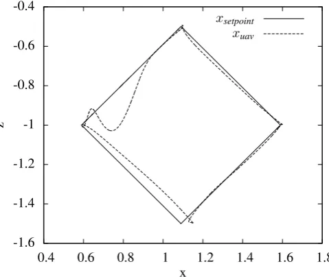
Lastly Figure 14 shows both an x-y and an x-z plot of the path tracking capabilities of the quadrotor UAV when docked. This also shows that the quadrotor UAV is not always capable of following the reference closely. However it remains stable and due to the robotic manipulator in contact with the wand.

-1 -0.8 -0.6 -0.4 -0.20 0.2 0.4 -0.5 -0.4 -0.3 -0.2 -0.1 0 0.3 0.4 0.5 0.6 0.7 0.8 0.9

0 20 40 60 80 100 120 140

x (m) y (m) z (m) t (s)

Free-flight tracking Docked tracking

xsetpoint xmeasured ysetpoint ymeasured zsetpoint zmeasured

Fig. 11. Path tracking of the quadrotor UAV with respect to the inertial frame,Fi.x denotes the forward direction,y the sideward direction and

z the height of the quadrotor UAV. Good tracking performance can be observed, both during free-flight tracking of the wand, docked tracking and idle free-flight.

VI. CONCLUSIONS

In this paper, we presented the design of a control archi-tecture for a flying hand and a mobile manipulation system. The flying hand consists of an unmanned aerial vehicle, a robotic manipulator and a gripper, which is grasping an object fixed on a vertical wall or a mobile one, attached to a wand controlled by a human. The control strategy is based on passivity-based techniques and has been shown to guarantee the asymptotic stability of the system in both simulations and in experimental tests.

REFERENCES

[1] AIRobots. [Online]. Available: http://www.airobots.eu

[2] D. Mellinger, M. Shomin, N. Michael, and V. Kumar, “Cooperative grasping and transport using multiple quadrotors,” in Proceedings of the International Symposium on Distributed Autonomous Robotic Systems, 2010.

[3] Q. Lindsey, D. Mellinger, and V. Kumar, “Construction of cubic structures with quadrotor teams,” in Proceedings of the Robotics: Science and Systems Conference, 2011.

[4] N. Michael, S. Kim, J. Fink, and V. Kumar, “Kinematics and statics of cooperative multi-robot aerial manipulation with cables,”University of Pennsylvania, USA, Technical Report, 2009.

[5] Q. Jiang and V. Kumar, “The inverse kinematics of 3-d towing,”

-40 -20 0 20 40 60 -40 -200 20 40 60 30 50 70 90 110

0 20 40 60 80 100 120 140

x (mm) y (mm) z (mm) t (s)

Free-flight tracking Docked tracking

xsetpoint xmeasured ysetpoint ymeasured zsetpoint zmeasured

Fig. 12. Path tracking of the end effector of the delta structure with respect to the base frame of the delta structure,Fb.xdenotes the height of the manipulator,y denotes the sideways movement andz denotes the forward motion away from the quadrotor UAV. Note that almost the whole workspace of the manipulator is used to compensate for the UAV’s offset to the setpoint as seen in Figure 11.

[6] A. Albers, S. Trautmann, T. Howard, T. Nguyen, M. Frietsch, and C.Sauter, “Semi-autonomous flying robot for physical interaction with environment,” in Proceedings of the IEEE Conference on Robotics Automation and Mechatronics, 2010.

[7] L. Marconi, R. Naldi, and L. Gentili, “Modeling and control of a flying robot interacting with the environment,”Automatica, vol. 47, no. 12, pp. 2571 – 2583, 2011.

[8] P. Pounds, D. Bersak, and A. Dollar, “Grasping from the air: hovering capture and load stability,” inProceedings of the IEEE International Conference on Robotics and Automation, 2011.

[9] P. Pounds and A. Dollar, “UAV rotorcraft in compliant contact: Stability analysis and simulation,” in Proceedings of the IEEE/RSJ International Conference on Intelligent Robots and Systems, 2011. [10] C. Korpela, T. Danko, and P. Oh, “MM-UAV: Mobile manipulating

unmanned aerial vehicle,”Journal of Intelligent & Robotic Systems, vol. 65, no. 1–4, pp. 93–101, 2012.

[11] “Ascending Technologies.” [Online]. Available: http://www.asctec.de/ [12] A. Keemink, M. Fumagalli, S. Stramigioli, and R. Carloni, “Mechan-ical design of a manipulation system for unmanned aerial vehicles,” inProceedings of the IEEE International Conference on Robotics and Automation, 2012.

[13] G. A. Kragten, “Underactuated hands - fundamentals, performance analysis and design,” Ph.D. dissertation, TU Delft, 2011.

[14] R. Murray, Z. Li, and S. Sastry,A mathematical introduction to robotic manipulation. CRC, 1994.

[15] N. Diolaiti, C. Melchiorri, and S. Stramigioli, “Contact impedance estimation for robotic systems,” IEEE Transactions on Robotics, vol. 21, no. 5, pp. 925–935, 2005.

[16] M. Fumagalli, R. Naldi, A. Macchelli, R. Carloni, S. Stramigioli, and L. Marconi, “Modeling and control of a flying robot for contact inspection,” inProceedings of the IEEE/RSJ International Conference on Intelligent Robots and Systems, 2012.

-1 -0.5 0 0.5 1 1.5 -2 -10 1 2 3 -1 -0.5 0 0.5 -2 -10 1 2

0 20 40 60 80 100 120 140

W and position (m) Fx (N) Fy (N) Fz (N) t (s)

Free-flight tracking Docked tracking

x y z

Fig. 13. Measured path of the wand (top) as well as the forces exerted by the wand on the manipulator system (bottom three).

[17] H. K. Khalil,Nonlinear Systems. Prentice Hall, 1996.

[18] N. Hogan, “Impedance control: An approach to manipulation,”Journal of Dynamic Systems, Measurement, and Control, vol. 107, no. 1, pp. 1 – 24, 1985.

[19] “20sim.” [Online]. Available: http://www.20sim.com

[20] “OptiTrack.” [Online]. Available: http://www.naturalpoint.com/ optitrack/

-0.42 -0.39 -0.36 -0.33 -0.3 -0.27

y

(m)

0.4 0.5 0.6 0.7 0.8

-0.8 -0.6 -0.4 -0.2 0 0.2

z

(m)

x (m) Setpoint

Measured

Setpoint Measured

Conclusions

The work presented in this research showed the design of a control

archi-tecture for a flying hand as well as a mobile manipulation system. Herein

the flying hand is composed of three subsystem; a quadrotor UAV, a robotic

manipulator and a gripper. For mobile manipulation a wand like object was

added to the system. This want had to be operated by a human being and

allowed for some insights into the interaction forces.

The proposed control architecture, a cascade of impedance controlled

subsystems, was shown to guarantee the asymptotic stability of the system

in theory, simulation as well as experiment for different states, i.e.

free-flight, docking to both a static and a dynamical object, and tracking a

certain trajectory whilst docked to the object being tracked, i.e. the wand.

The design of the gripper required for the research proved to work as

intended. Although from a practical point of view, the proposed feedback

control proved to be difficult due to the fact that full determination of the

phalange location is impossible by means of the 3d tracking system and the

absence of information about the physical object.

Unfortunately the idea of using a second UAV, i.e. the Ducted Fan, to

perform some cooperative flying and grapsing proved difficult due to the

instability of the platform. However the principle of cooperative grapsing

has been illustrated by means of the experiments with the wand, provided

a platform with a high attitude control is used.

Recommendations for future work

Althought the system is shown to work, some improvements and/or future

extensions might be possible:

•

Determine whether the proposed architecture works with a second

UAV as well;

•

Get the Ducted Fan to fly more stable, i.e. by equiping the ducted fan

with onboard gyroscopes for a low level hard real-time attitude control

loop;

•

The gripper can be extended as well to support a VSA which enables

handling of different object stiffnesses with a variable passive spring

in stead of by means of control. Also support for pinching might be

desirable;

•

In order to apply all the proposed stratigies outside the external visual

system should be removed and IMUs be used instead.

A

Gripper design

The research presented in this report requires a gripper capable of interacting

actively with the environment. The design, from concepts to a physical

system, of such a gripper is detailed out below. At first several concepts are

thought up or reviewed and modelled. Afterwards one design is chosen and

physically created.

A.1

Requirements

The gripper should be mountable on the side of an aerial vehicle. This

imposes several limitations. Due to the off centre location the total weight

should be kept to a minimum. Also if possible the weight should be evenly

distributed over the UAV in order to keep it statically balanced. With

this in mind and taking goals of the project into account as well, a list of

requirements can be formulated:

•

The gripper should be underactuated due to weight constraints;

•

Form closure should be achievable;

•

Various object sizes, shapes and stiffnesses should be possible;

•

Easily constructible.

A.2

Concepts

With the list of requirements in mind three concepts were thought up. All

of these are modelled using 20-sim to figure out their feasibility and

concor-dance to the requirements. In order to model the gripper concepts several

parts had to be modelled from scratch. Among these an element to resemble

physical contact between two objects was created and based on the

Hunt-Crossley model with friction. Also several tendon structures were made as

well as spring structure between two joints.

In the end all three concepts were modelled successfully which enabled

comparison of them all and one could be chosen for physical creation.

Since form closure should be achievable a minimum of three fingers is

required. Also all of the concepts are tendon driven to help with weight

distribution. For convenience and clarity only one finger is drawn for each

concept.

A.2.1

Concept One

A schematic of the first concept can be found in Figure 1. The principle

behind the concept is that the rotational springs always tend to close the

finger, while the tendon pulling on the outmost phalange is used to keep

the finger and thus the gripper open. The amount of force exerted on the

tendon determines the configuration of the finger due to the equilibrium of

forces

F

+

F

+

F

= 0

(1)

so the system is force driven. Also the maximum amount of force that can

be exerted on the environment is fully determined by the rotational springs.

Figure 1: Schematic overview of one finger of the first gripper concept. The

rotational springs ensore the finger closes, while pulling the tendon opens it.

An advantage

of this system is that form closure is ensured.

Disadvantages

of such a system is the fact that the force exerted on the

environment is fully determined by the rotational spring force and the fact

that the tendon is always loaded which in turn means that the motor will

always have to deliver a force to the system.

A.2.2

Concept Two

The second concept relies on the ratio between in- and output pulleys of

each phalange and the previous one and is loosely based on the work of M.

Wassink. This means the system is position driven. In fact the trajectory

of each of the phalanges is in fact fully determined due to these ratios. A

schematic overview of the system can be found in Figure 2.

Advantages

of this system are that it allows for controlled actuation back

and forth and an unloaded tendon.

A disadvantage

is that the motion profile is fully defined by the pulley

ratios. Therefore form closure in terms of full contact with the environment

cannot be guarenteed.

Figure 2: Schematic overview of one finger of the second gripper concept.

The ratio between in- and output pulleys of each phalange fully determines

the trajectory of the phalanges.

A.2.3

Concept Three

The third and final concept can be found in Figure 3 which is based on a

proposal of Gert A. Kragten. This system is driven by tendons connected

to the vertical phalange, imposing a rotation. All the other phalanges can

rotate freely. The spring ensures the outmost phalange stays open untill the

first bottom phalange hits the environment. When this occurs the outmost

one rotates inward ensuring form closure.

Figure 3: Schematic overview of one finger of the third gripper concept. The

spring between the phalanges keeps the outmost phalange in its open state

untill the first bottom phalanges is in contact with the environment.

Advantages

of this concept are that it ensures form closure, is drivable

in both directions and it requires a low operating force, slightly higher than

the spring force is enough to close the gripper completely.

A disadvantage

is the fact that the full trajectory of the phalanges is not

fully determined by the freedom in rotation of most of the joints.

A.2.4

Comparison

In order to choose a concept, the concordance to the requirements for each

is displayed in Table 1.

Form closure

Variable objects

Constructibility

Concept One

+

+

0

Concept Two

-

0

+

Concept Three

+

+

+

Table 1: Comparison of concepts based on requirements

This table clearly shows that concept three has all the desired

func-tionability. Therefore this design is chosen and converted to a physical

prototype.

A.3

Physical realisation

This chapter describes the physical realisation of the chosen system. In order

to do so both the gripper itself and a motor housing need to be designed as

well as a connection in between. This to ensure a proper weight distribution

of the subsystem over the UAV. The motor housing is connected to the

gripper by means of bowden cables made of a steel inner cable coated with

teflon, a teflon tube and a flexible steel outer shell.

A.3.1

Gripper

In order to realise the gripper itself physically the model needs to be adapted

slightly. The main reason for this is that the current driving mechanism

might hit objects in the gripper, which is unwanted. To overcome this

problem the actuation is done via a rod connected to a pulley. The rod is

in turn connected to the top joint of the vertical phalange. In essence this

imposes the same rotation on the vertical phalange and thus results in the

same workings. The result can be found in Figure 4

The dashed line in the figure shows how the tendon passes through the

subsystem. The reason it crosses in the middle is to change the rotation

of the top with respect to the bottom in order to ensure both top and

bottom fingers close when bottom cable is pulled and open when the top

cable is pulled in Figure 4. Effectively, this ensures a push-pull configuration

allowing for both controlled opening and closing of the gripper.

A.3.2

Motor housing

The motor housing forms an interconnection between the motor and the

tendons. To achieve this connection a pulley is used to which both the push

and pull cable is connected. The technical drawing hereof can be seen in

Figure 4: Technical drawing of the gripper along with the bowden cables

drawn in (dashed line).

Figure 5 as well as the tendon connections. Note that bottom cable actually

goes behind the pulley from this point of view.

Figure 5: Technical drawing of the motor housing along with the bowden

cables drawn in (dashed line).

B

Ducted fan manual

The ducted fan is an unmanned aerial vehicle (UAV) designed by the

Uni-versity of Bologna. The aim of this article is to give a more in depth look

into the inner workings of this UAV both from a hardware and software

point of view. Also some insight is given into the mathematics behind the

vehicle and some remarks about simulations will be made as well as some

conclusions drawn.

B.1

Hardware

The hardware of the ducted fan can be divided into a mechanical and an

electronical part.

B.1.1

Mechanics

From a mechanical point of view the ducted fan is composed of the following

parts:

•

A cylindrical duct that serves as the main body of the vehicle to which

everything is connected;

•

A main rotor that spans 280 millimeters, used for thrust generation;

•

Eight vanes that are connected beneath the main rotor and can be

used to direct the airflow.

The idea behind this mechanical setup is that by forcing air through the

cylindrical duct by means of the main rotor lift is generated. In turn the

vanes direct the flow of air in order to keep the vehicle upright as well as to

steer it to a desired location.

B.1.2

Electronics

The electronics used in the system are the following:

•

An Arduino ATMega2560 that is in charge of low level control;

•

A Polulu Mini Maestro 12 board that is used to control all the

actua-tors by means of its servo outputs;

•

A Scorpion SII-3026-1190KV Brushless Motor that drives the main

rotor;

•

An Electronic Speed Controller (ESC) which controls the main rotor’s

speed based on the servo output it receives from the Polulu board;

•

Eight Digital BB Carbon Gear Servos (HG-D202HB) to control the

angle of the eight vanes;

•

An xBee on an xBee Adapter for communication with the rest of the

world;

•

An Ultimate Battery Eliminator Circuit (UBEC) to generate a stable

5

V

line;

•

A 5S Lithium Polymer battery of 3400 mAh to supply power to the

system;

•

An AttoPilot, used to measure the current delivered by the battery

pack to the system as well as the driving voltage.

The way all these different electronical components are connected to each

other can be seen in Figure 6.

Figure 6: The interconnection of all the different electronical components

B.2

Software

In order to get the complete system to work, both low (embedded) and high

level software is required. A schematic overview of the system flow can be

found in Figure 7.

The low level software takes the form of C++ code for the Arduino that

reads input messages relayed by the xBee over a TTL serial connection. The

contents of these messages are setpoints for both the vanes and the main

rotor. After some checking the parsed messages are relayed over another

3D tracking

Ground station

Aerial vehicle

xBee

xBee

High level

P

ose

estimation

control

Figure 7: Schematic overview of the signal flow for the control of the ducted

fan. Dashed lines indicate optional communication.

TTL serial connection to the Polulu board that in turn sets the appropriate

servo outputs to the appropriate values. This all occurs at 50 Hz.

Optionally the Arduino can read out the sensed values from the AttoPilot

and send these back to the high level control via the xBee. In practise the

maximum available communication rate of the xBee (57600 kbps) deemed

to low for this to happen simultaniously.

The high level software part of the system is constructed in Matlab

Simulink and run via Windows Real-Time Target. This peace of software

receives input from both an OptiTrack system, used to determine position

and orientation of the UAV, as well as a PS3 controller, needed to steer

the UAV. These inputs yield setpoints for the UAV which are converted

to the appropriate format (servo values) and send as a stream to the xBee

connected to the ground station.

B.3

Control & Simulation

In this section the dynamics and its control will be discussed briefly. Also

some notes on simulation will be given.

B.3.1

Dynamics

The ducted fan is like the quadrocopter an underactuated system, since it

has only four control inputs, i.e. the thrust

T

, and the angles

α

,

β

and

γ

of

the vanes, and six degrees of freedom (DoF). Due to the mechanical design of

the ducted fan, a net torque as well as force can be applied in any direction

by varying the angles of the vanes. The mapping between the generated

thrust of the rotor and the angles of the vanes and the total wrench exerted

DuctedFan

Object

F

F

F

p

, R

p

, R

f

, M

Figure 8: The ducted fan UAV and its reference frames.

on the UAV’s c.g. is given by

















M

M

M

f

f

f

















=

















0

dT k

0

0

0

0

dT k

0

0

0

0

2

T k

0

0

dT k

0

0

dT k

0

0

1

0

0

0

























T

α

β

γ









(2)

where

d

is the distance between the UAV’s c.g. and the centre of the

vanes, and

k

and

k

the ratios between the propeller reaction torque and

generated thrust. Using this and Figure 8 as a visual reference, the full

dynamics of the UAV can be described by

m

v

˙

=

m

g

z

ˆ

+

R

f

+

R

R

f

J

ω

˙

=

−

ω

×

J

ω

+

M

+

M

+

R

M

+

R

f

×

p

(3)

where ˙

ω

and

ω

are the rotational velocity and acceleration of the UAV

with respect to the inertial frame,

F

, expressed in the ducted fan frame,

F

, respectively; ˙

v

the linear acceleration of the UAV’s c.g. in

F

;

f

the

control force input and

f

the forces due to external input.

R

denotes a

rotation of frame

a

with respect to frame

b

and

p

a

denotes a translation of

frame

a

with respect to frame

b

.

B.3.2

Control

A similar approach as with the quadrotor can be applied to the ducted fan,

i.e. assuming a high attitude control authority which reduces the ducted

fan’s system dynamics in Equation 3 to

m

v

˙

=

m

g

z

ˆ

+

R

f

+

R

R

f

(4)

where

R

d

R

f

is the external force input due to the interaction with the

other UAV via the bar shaped object. By letting

R

f

=

u

−

m

g

z

ˆ

(5)

the system equation is reduced to something similar as the equations for the

quadrotor UAV and the same further analysis applies.

B.3.3

Simulation

Using the above dynamics and control several simulations were done

includ-ing cooperative flyinclud-ing with a quadrotor UAV. All of these seemed stable

up to some level of disturbance. Also the path tracking capabilities were

explored and seemd to be working sufficiently.

However when trying out the real hardware and control, the system

turned out to be less stable than expected. The assumption of high attitude

control, upon which the control architecture is based, turned out to be not

valid. The cause of this might be due to the fact that the whole control

architecture is run off-site, i.e. on a PC near the ducted fan and setpoints

are relayed to it via xBee. This creates a lot of delay in the feedback and

therefore causes instability.

In order to overcome these problems moving some of the control to the

ducted fan itself by means of some gyroscopes or an IMU for instance, the

high attitude controller can be run at a much higher frequency and have less

delays as well.