MR quantification of cerebral ventricular volume using a semiautomated algorithm

MR Quantification of Cerebral Ventricular Volume Using a

Semiautomated

Algorithm

L.A. Johnson, J.D. Pearlman, C. A. Miller, T. I. Young, and K. R. Thulborn

PURPOSE: A semiautomated border identification algorithm, insensitive to user bias, is evaluated

for accuracy and speed in the measurement of ventricular volumes from three-dimensional MR images. METHODS: A three-dimensional gradient-echo technique was implemented on a Signa

clinical imaging system. Data from phantoms and patients were analyzed for volume using a

segmentation algorithm designed with: 1) correction for partial volume averaging; 2) insensitivity

to user bias; and 3) speed. Accuracy, precision, and intra- and interobserver variability were

determined. RESULTS: Average error for phantom studies was 4% to 6%, or 1 to 2 cc across the

volumes, which ranged from normal to mild hydrocephalus (<60 cc). Patient studies showed intra-and interobserver error of 2.3% and 7.8%, respectively. The correction for partial volume averaging

resulted in a threefold decrease in error. Data were acquired and reconstructed within 7 minutes.

Experienced radiologists required less than 15 minutes to perform each analysis. CONCLUSIONS: This algorithm allows accurate measurement of ventricular volumes in an efficient, minimally supervised manner.

Index terms: Brain, ventricles; Brain, volume; Brain, occipital lobe; Brain, magnetic resonance; Magnetic resonance, 3-D; Degenerative brain disease

AJNR 14:1373-1378, Nov/Dec 1993

Accurate determination of cerebral ventricular

volumes

can be important for the diagnosis of

hydrocephalus

and can provide

important

follow-up

information in patients with

intraventricular

shunts.

Changes in cerebrospinal fluid (CSF)

ven-tricular

volume also have been shown to have

clinical significance in patients with Alzheimer

disease

(1-3)

and benign intracranial

hyperten-sion

(4). However, the majority of studies in the

literature

on measuring cerebral ventricular size

have

been conducted with computed

tomogra-phy,

often using linear or area measurements as

indices

of ventricular volume (3,

5-14).

Those

magnetic

resonance studies which measured

ac-tual

volumes were done with skip areas (

15-18)

with

lower resolution than magnetic resonance

Received May 27, 1992; revision requested September 3, received November 16, and accepted November 23.

This work was supported by National Institutes of Health Grant ROJ HL45176 and by the Whitaker Foundation.

All authors: Nuclear Magnetic Resonance Center, Massachusetts Gen -eral Hospital, 13th St, Bldg 149, Charlestown, MA 02129. Send reprint

requests to Keith R. Thulborn, MD, PhD.

AJNR 14:1373-1378, Nov/Dec 1993 0195-6108/93/1406-1373 © American Society of Neuroradiology

can provide (

19-22)

or with long imaging or

analysis times

(1, 23-25)

that are not practical

for routine clinical applications.

The purpose of the present study was to

test

a semiautomated computer algorithm able to

calculate cerebral ventricular volume rapidly with

minimal operator

input

and to correct for partial

volume effects.

Methods

Phantom Studies

Phantom Construction. A diagram of the phantom is shown in Figure 1. Three paraffin cylinders were con-structed with volumes of 12.3 ± 0.5 ml (±1 SD, n

=

5), 29.2 ± 0.2 ml (±1 SD, n

=

5), and 58.6 ± 0.7 ml (±1 SD, n

=

8). These volumes were determined by multiple measurements of the weight of water displaced by the phantoms; the average measurement was used as the true volume of the phantoms. These volumes approximate the range of ventricular volumes encountered in patients with normal to mildly enlarged ventricles, as reported in both the pathology and imaging literature (20, 26-29). The paraffin cylinders were suspended in water titrated with gadopentetate dimeglumine (Magnevist, Berlex Laborato -ries, Inc, Wayne, NJ), to obtain the same contrast ratio between the water and paraffin as that between brain

1374 JOHNSON

Fig. 1. Schematic representation of the paraffin-water phan-tom.

The paraffin cylinders (A, 8, and C) were suspended on cotton thread to ensure that water fully surrounded them. Volumes are 58.6 (A), 29.2 (B), and 12.3 (C) mL measured as described in

Methods.

parenchyma and CSF in normal brains imaged with the same gradient-echo, three-dimensional (3D) pulse sequence technique. The final concentration of gadolinium was not determined. The paraffin blocks were suspended on cotton threads in the water to ensure that water completely surrounded the cylinders. The solid paraffin cylinders avoided a physical separation between the two compart-ments that would artificially aid in boundary determination during image analysis.

Data Acquisition. A customized, gradient-echo 3D pulse sequence on the Signa 1.5-T imager (GE, Milwaukee, Wis; software version 3.38) was used to acquire 28 contiguous sections. The current software release (version 4. 7) for Signa has a commercial equivalent of this sequence (SPGR), which has a shorter echo time (5 msec) than that available with the 3.38 software. Scan parameters were chosen for optimal brain parenchyma-to-CSF contrast and optimal signal-to-noise ratio. The parameters used were 50/9/1 (repetition time/echo time/excitations), flip angle 50°, and field of view 24 em. Both 256 X 128 and 256 X 256 matrices were acquired for the phantom. Data sets with section thicknesses of both 3 and 5 mm were obtained on phantoms. Only 5-mm thick sections and field of view 128 X 256 were obtained on patients. Images were obtained in the coronal plane orthogonal to and at 30° to the long axis of the phantoms to provide different partial volume contributions. Patient studies were performed in the coronal plane.

Data Analysis. Images were analyzed on a Sun 4 work station (Sun Microsystems, Mountain View, Calif) using a semiautomated image segmentation package which reads data from any format and identifies borders between two contiguous compartments sampled by the operator as described below.

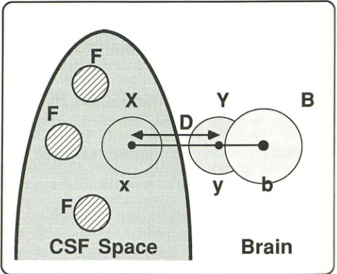
Before beginning the analysis, the operator selects sev-eral circular regions in the area of pure foreground (regions labeled Fin Fig 2) to define the average intensity value of the foreground, averaged over the selected regions. This

AJNR: 14, November/December 1993

number for average intensity of the foreground is identified as pure F. To define a given boundary, such as that between CSF and brain parenchyma, the operator selects an area on each side of the desired border by placing the cursor at the appropriate positions (points x and y in Fig 2). The computer then automatically samples a circular region around each point, with a radius equal to one-third of the distance between the two selected points (circles labeled X and Y in Fig 2). By comparing the distribution of signal intensities in each of the two circular regions, the computer determines the border value, which results in the least number of misclassified pixels between the two popula-tions. The border is superimposed on the displayed image, and the computer automatically classifies pixels or fractions of pixels which contribute to the total volume based on the signal intensity of each, compared with the signal intensities of the background and foreground. To provide a correction for partial volume averaging, the pure background must be sampled. This is done automatically by the algorithm by choosing a third point (labeled b in Fig 2) to estimate locally the background intensity. This point is located a distance half the distance between the two original points away from the previously selected point, y. A circular area with the radius equal to half the distance between the two original points is sampled (circle labeled B in Fig 2), gen-erating an average signal intensity value (BSI) for the pure background region. Because circle Y is close to the desired border and contains voxels with partial voluming, it cannot substitute for circle B. The operator then confirms the region of interest (ROI) which has been outlined by the

8

Brain

Fig. 2. Scheme for use of border-drawing algorithm as de-scribed in detail in the text.

[image:2.612.56.300.81.262.2] [image:2.612.318.561.430.628.2]

AJNR: 14, November /December 1993 VENTRICULAR VOLUME 1375

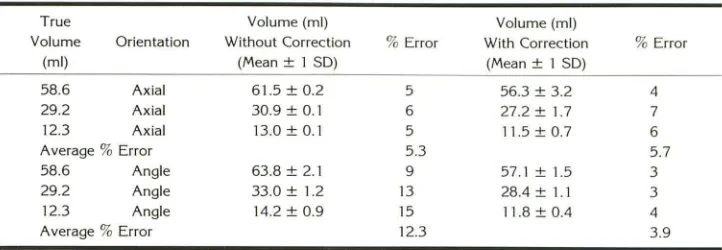
TABLE 1: Phantom volumes with and without correction for partial volume averaging

True Volume (ml)

Volume Orientation Without Correction

(ml) (Mean± 1 SD)

58.6 Axial 61.5 ± 0.2

29.2 Axial 30.9 ± 0.1

12.3 Axial 13.0± 0.1 Average % Error

58.6 Angle 63.8 ± 2.1 29.2 Angle 33.0 ± 1.2 12.3 Angle 14.2 ± 0.9 Average % Error

contour map, and the volume contribution automatically

determined by the computer. Using both the mean fore-ground signal intensity (FSI) and the mean BSI, corrections

for partial volume averaging in the ROI chosen by the operator are made according to the following formula:

volume * BSI - mean signal intensity of the ROI/BSI -FSI

=

corrected volume.

The difference in average signal intensity between the background and the ROI as a fraction of the difference in average signal intensity between the background and the foreground is multiplied by the area in pixels of the ROI to obtain a corrected volume. This accounts for partial volume

averaging and is scaled by the pixel dimensions and section thickness. In summary, once the operator has selected the

initial two areas of interest on either side of the desired border (points x and yin Fig 1 ), the border is automatically determined, and the region and corrected volume of the

ROI are calculated in less than 1 sec. The computer uses the original image intensity data for calculation of the borders and the partial volume correction. The computer program also allows manual modification of any part of the border, if desired. The volumes for each region are

automatically summed over the entire 3D stack to yield a final total volume after all sections have been analyzed.

Patient Studies

Six adult patients were examined with customized, gradient-echo 3D pulse sequence during a routine brain screening protocol. The average age of the patients was 50 years, with a range of 28 to 78. There were three men and three women. Two patients had a diagnosis of ventric-ulomegaly associated with cerebral atrophy: one had non-specific subarachnoid enlargement with normal ventricles,

one had an area of focal gliosis with normal ventricles, and two patients had normal brain MR examinations. Informed consent was obtained from all participants.

Data acquisition and analysis were performed using the techniques outlined for the phantoms. To determine the

average signal intensity representing pure foreground value

of CSF, ROis were sampled by the operator from several coronal images of the lateral ventricles at their widest diameter.

Volume (ml)

%Error With Correction

(Mean± 1 SD)

5 56.3 ± 3.2

6 27.2 ± 1.7

5 11.5 ± 0.7

5.3

9 57.1 ± 1.5

13 28.4 ± 1.1

15 11.8 ± 0.4 12.3

Results

Phantom Studies

%Error

4 7 6 5.7 3 3 4 3.9

Results of phantom stud

i

es both with and with

-out correction for partial volume averaging are

shown in Table 1

.

The mean error with the partial

volume averaging correction was 2 mL for the

axial scans and 1 mL for the 30° angle scans

.

The volumes from axial images

,

taken in a plane

perpendicular to the

long axis of the phantoms

,

do not show a significant difference before and

after partial volume cor

r

ection (5.3

%

versus

5

.

7

%

)

.

Presumably this is because there is very

little partial volume averaging in the axial images

of the phantoms. One would expect only a small

amount of volume averaging in the pixels at the

edges of the phantom border

,

and in this partic

-ular phantom the end section volume averaging

was minimal because the phantom length of

6 em allowed the acquisition of 12 5-mm sections

with minimal volume averaging at the ends

.

How

-ever

,

in the 30° angle images

,

in which partial

volume averaging effects are larger because of

the oblique angle, the reduction in error when

using the partial volume correction was signifi

-cant and represented a threefold decrease in the

average error (from 12

.

3

%

to 3.9

%

)

.

Although the volumes obtained without the

partial volume corrections were higher than the

true volumes (Table 1

,

column 3)

,

the volumes

obtained with the partial volume corrections were

slightly lower (Table 1

,

column 5)

.

In the

phan-toms with high-contrast borders

,

Gibbs r

i

nging

artifact along the borders resulted in lower

cal-culated volumes becaus

e

of ov

e

restimation of the

true signal intensity valu

e

of the inner reg

i

on.

Because of the sharper borders and more severe

ringing artifact

i

n the axial phantoms

,

this artifact

contributed to the h

i

gher perc

e

ntage error of axial

[image:3.612.124.485.92.217.2]

1376 JOHNSON AJNR: 14, November /December 1993

TABLE 2: The effect of voxel size on the percent error of phantom volume measurements

ST" Matrix Voxel Size Timeb Large< Mediumd

%Error Small• %Error %Error

(mm) Size (mm3

) (min) Phantom Phantom Phantom 5 256 X 128 8.79 6:35 57.3 ± 1.9 2.3 29.0 ± 0.5 0.5 12.0 ± 0.3 2.3 3 256 X 128 5.27 12:45 57.8 ± 1.6 1.4 29.6 ± 0.5 1.3 12.5 ± 0.3 1.4 5 256 X 256 4.39 10:55 59.0 ± 0.4 0.1 28.8 ± 1.2 1.3 11.3 ± 0.6 5.3 3 256 X 256 2.64 22:05 58.6 ± 0.1 <0.1 29.3 ± 0.1 0.5 12.3 ±0.4 <0.1

Note.-Each set of images was analyzed three times by a single individual. ' Section thickness.

b Time represents the total data acquisition time and image reconstruction time. c Volume = 58.6 mi.

d Volume = 29.2 mi.

• Volume = 2.3 mi.

The time required for computational analysis

of the phantoms was approximately 2 seconds per section, with a total operator time, including

review and selection of pure foreground and

points x,y for each of 28 sections, of less than 10 minutes.

To calculate interobserver variability, results

were compared between two observers. There

was no significant difference in the results (P

>

.05). To test the effect of varying the voxel size on measurement errors of the phantom volumes, images were taken at a 30° angle with four different voxel sizes. The partial volume averag-ing correction was used. Five- and 3-mm sections

were taken with both 256 X 128 and 256 X 256

matrices. The results are shown in Table 2.

Although the percent error is lower for the

smaller voxel sizes, application of the Student t

test shows that there is no significant difference

between the calculated volumes when using

dif-ferent voxel sizes and partial volume correction

(P

>

.05). However, although the calculated

vol-umes are not significantly different, there is a

substantial increase in the time of acquisition and reconstruction for the smaller voxel sizes; 6

min-utes and 35 seconds for the largest voxels,

com-pared with 22 minutes and 5 seconds for the

smallest voxel.

Clinical

Studies

Imaging was performed in the coronal plane

because of its perpendicular orientation to the

long axis of the lateral ventricles, which comprise

the largest portion of the cerebral ventricular

system. For a fixed section thickness, less sec-tion-to-section contour variation is seen in the lateral ventricles using the coronal plane as com-pared with the variation seen in the axial and sagittal planes.

TABLE 3: lntraobserver coefficient of variation

Coefficient of Ventricular 1st 2nd 3rd

Variation Volumes Analysis Analysis Analysis

(%)

Right lateral 21.3 23.2 22.7 4.4

Left lateral 21.8 20.1 21.5 4.3

Third 1.8 1.6 2.6 2.7

Fourth 1.5 2.1 1.7 1.7

Total 46.4 47.0 48.5 2.3

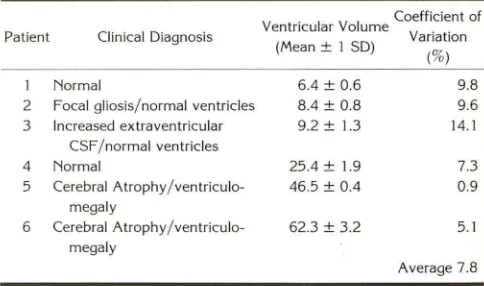
TABLE 4: lnterobserver coefficient of variation

Coefficient of Ventricular Volume

Variation Patient Clinical Diagnosis

(Mean± 1 SD)

(%)

1 Normal 6.4 ± 0.6 9.8

2 Focal gliosis/normal ventricles 8.4 ± 0.8 9.6 3 Increased extraventricular 9.2 ± 1.3 14.1

CSF /normal ventricles

4 Normal 25.4 ± 1.9 7.3

5 Cerebral Atrophy /ventriculo- 46.5 ± 0.4 0.9 megaly

6 Cerebral Atrophy /ventriculo- 62.3 ± 3.2 5.1 megaly

Average 7.8

In the calculation of CSF ventricular volume for six patients, the intraobserver coefficient of

variation determined from three calculations

per-formed at separate points in time on one patient

was 2.3% (Table 3), whereas the interobserver

variation determined from examination of six

patient scans by three experienced observers was

7.8% (Table 4). Although the number of this

preliminary study is small, it is clear that for patients with the highest ventricular volumes

(2'::25 mL), which could be expected in

hydro-cephalus, the error is even lower (4%) than when

the patients with normal ventricular volumes are included.

For a brain study, the computational analysis

[image:4.612.125.490.97.171.2] [image:4.612.317.559.265.357.2] [image:4.612.317.559.389.532.2]

AJNR: 14, November /December 1993

requiring an experienced operator a total of 15 minutes to analyze an entire brain with ven-tricles covering 18 sections. This total time in-cludes loading the program, reading in the

im-ages, sampling the pure foreground, and selecting

x and y points for the ventricular border for each section and confirming the computer-selected ROI.

Discussion

The volumetric study of phantoms demon-strates that volume averaging contributes signif-icantly to error when using a thresholding tech-nique, and that this error can be dramatically improved when correction is made for partial volume averaging. Phantom studies also confirm that it is reasonable to use larger voxel sizes for

cerebral ventricular volume determination, espe

-cially when clinical imaging time is limited.

The range of cerebral ventricular volumes de

-termined from our patient studies is consistent

with published values

(20, 26

-

29).

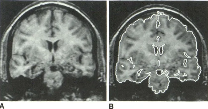
Because the

3D volume technique covers the entire ventricular system, precise alignment of the patient in the scanner from examination to examination is not required in order to compare results of ventricular volume analysis over time. We note that Figure 3 shows segmentation of the brain as the algo-rithm finds all tissue and CSF borders. Only the ventricles are selected in these studies. Brain volume can be measured in the same way as ventricular volume with this algorithm, and such applications will be presented elsewhere. Sepa-ration of gray and white matter also can be achieved with this algorithm, but the acquired data must be optimized for gray and white matter contrast.

A

8

VENTRICULAR VOLUME 1377

The errors in data acquisition are as follows.

Gibbs ringing artifact, resulting from the contrast between the water doped with gadolinium and

the paraffin, is more pronounced in the axial

images than in those oriented at a 30° angle to the long axis of the phantoms due to the higher

contrast borders. A multisection contiguous 2D

acquisition will have errors associated with the shape of the section profile, which is less impor-tant in a 3D acquisition. The difficulty in ensuring

that identical sections, necessary for 2D imaging,

are acquired for each study is obviated by 3D

imaging. Magnetic susceptibility is another source

of error, especially around air-tissue interfaces.

This error is reduced with use of the short echo

time of 9. Patient motion is also a source of error.

The data acquisition time of less than 4 minutes

minimizes voluntary patient motion. Motion of

the CSF is greatest in the fourth ventricle and the

aqueduct, which appear in only a few sections in

the coronal orientation and represent ventricles that do not contain a large portion of the total

CSF ventricular volume (Table 3).

Sources of error in data analysis include poten-tial inaccuracy of the border determined by the algorithm. Errors arising from the choice of re

-gions x and y (Fig 1) by the operator were found to be 1% to 2% when tested in phantoms. Other sources of error included variations in the sam-pling regions chosen by the algorithm to

deter-mine background brain intensity (the region

la-beled B, based on the choice of x and y in Fig 1 ), variations in the regions chosen to represent pure CSF (regions labeled F in Fig 1 ), and manually drawn variations in the border, chosen when the

automatically drawn borders need closure in

or-der to outline a ventricular region accurately. This

last error can occur around the third ventricle

Fig. 3. A selected coronal image (A) from a 3D set of a human brain obtained using a customized, gradient-echo 3D pulse sequence (equivalent to the com-mercial SPGR sequence available from GE in the Signa version 4. 7 software but with a longer minimum echo time) and the same image (B) segmented for ven -tricular volume measurement. Only the regions containing CSF are selected for the ventricular volume measurement once the border is drawn, although the

[image:5.612.55.393.558.736.2]

1378 JOHNSON

because of poor contrast between third

ventric-ular CSF and quadrigeminal plate cisterns. These errors are all assessed by the intra- and interob-server variations calculated from the analysis of

patient studies and are of an acceptable

magni-tude (coefficient of variation 2.3% and 7.8%,

respectively, as shown in Tables 3 and 4).

Measurement of ventricular volume can be

made accurately and rapidly with the described

algorithm with minimal supervision.

References

1. Rusinek H, de Leon MJ, George AE, et al. Alzheimer disease: m eas-uring loss of cerebral gray matter with MR imaging. Radiology

1991;178:109-114

2. George AE, de Leon MJ, Rosenbloom S, et al. Ventricular volume and cognitive deficit: a computed tomographic study. Radiology

1983; 149:493-498

3. de Leon MJ, George AE, Reisberg B, et al. Alzheimer's disease: longitudinal CT studies of ventricular change. AJNR: Am J Neuror a-diol 1989; 10:371-376

4. Reid AC, Teasdale GM, Matheson MS, Teasdale EM. Serial ventricular volume measurements: further insights into the aetiology and path

-ogenesis of benign intracranial hypertension. J Neural Neurosurg

Psychiatry 1981 ;44:636-640

5. Evans WA. An encephalographic ratio for estimating the size of the

cerebral ventricles. Am J Dis Child 1942;64:820-830

6. Hanson J, Levander B, Liliequist B. Size of the intracerebral ventricles as measured with computer tomography, encephalography, and

echoventriculography. Acta Radio/1975;346 (suppl):98-106 7. Hahn FJY, Rim K. Frontal ventricular dimensions on normal

com-puted tomography. AJR: Am J Roentgeno/1976;126:593-596 8. Synek V, Reuben JR, Du Boulay GH. Comparing Evans' index and

computerized axial tomography in assessing relationship of ventric-ular size to brain size. Neurology 1976;26:231-233

9. Gyldensted C. Measurements of the normal ventricular system and hemispheric sulci of 100 adults with computed tomography. Neuro

-radiology 1977; 14:183-192

10. Haug G. Age and sex dependence of the size of normal ventricles on

computed tomography. Neuroradio!ogy 1977;14:201-204

11. Pfefferbaum A, Zatz LM, Jernigan TL. Computer-interactive method for quantifying cerebrospinal fluid and tissue in brain CT scans:

effects of aging. J Comput Assist Tomogr 1986;10:571-578 12. McArdle CB, Richardson CJ, Nicholas DA, Mirfakhraee M, Hayden

CK, Amparo EG. Developmental features of the neonatal brain: MR imaging. Radiology 1987; 162:230-234

AJNR: 14, November/December 1993

13. Gooskens RHJM, Gielen CCAM, Hanlo PW, Faber JA, Willemse J. Intracranial spaces in childhood macrocephaly: comparison of length measurements and volume calculations. Dev Med Child Neural 1988;30:509-519

14. Rossi A, Stratta P, Gallucci M, Passariello R, Casacchia M. Quantifi-cation of corpus callosum and ventricles in schizophrenia with nuclear magnetic resonance imaging: a pilot study. Am J Psychiatry

1989;146:99-101

15. Gada M, Hughes CP, Danziger W, Chi D, Jost G, Berg L. Volumetric measurements of the cerebrospinal fluid spaces in demented subjects and controls. Radiology 1982; 144:535-538

16. Jernigan TL, Press GA, Hesselink JR. Methods for measuring brain morphometric features on magnetic resonance images. Arch Neural 1990;47:27-32

17. Cramer GD, Allen Dl, DiDio LJA. Volume determinations of the

encephalic ventricles with CT and MRI. Surg Radio/ A nat 1990; 12: 59-64

18. Tanna NK, Kahn Ml, Horwich DN, et al. Analysis of brain and cerebrospinal fluid volumes with MR imaging: impact on PET data correction for atrophy. Radiology 1991; 178:123-130

19. Penn RD, Belanger MG, Yasnoff WA. Ventricular volume in man computed from CAT Scans. Ann Neural 1978;3:216-223

20. Brassow F, Baumann K. Volume of brain ventricles in man determined by computer tomography. Neuroradio!ogy 1978; 16:187-189 21. Condon BR, Patterson J, Wyper D, et al. A quantitative index of

ventricular and extraventricular intracranial CSF volumes using MR imaging. J Comput Assist Tomogr 1986;10:784-792

22. Grant R, Condon B, Lawrence A, et al. Human cranial CSF volumes measured by MRI: sex and age influences. Magn Reson Imaging

1987;5:465-468

23. Lim KO, Pfefferbaum A. Segmentation of MR brain images into cerebrospinal fluid spaces, white and gray matter. J Comput Assist

Tomogr 1989; 13:588-593

24. Ashtari M, Zito JL, Gold Bl, Lieberman JA, Borenstein MT, Herman PG. Computerized volume measurement of brain structure. Invest

Radio! 1990;25: 798-805

25. Kahn Ml, Tanna NK, Herman GT, et al. Analysis of brain and cerebrospinal fluid volumes with MR imaging. Radiology

1991;178:115-122

26. Last RJ, Tompsett DH. Casts of the cerebral ventricles. Br J Surg

1952;40:525-543

27. Schwartz M, Creasey H, Grady CL, et al. Computed tomographic analysis of brain morphometries in 30 healthy men, aged 21 to 81 years. Ann Neural 1985; 17:146-157

28. Takeda S, Matsuzawa T. Age-related change in volumes of the ventricles, cisternae, and sulci: a quantitative study using computed tomography. JAm Geriatr Soc 1985;33:264-268