Optimization of the BUbiNG web craler

(1)

Thesis Applied Mathematics

Faculty of Electrical Engineering, Mathematics and Computer Science (EEMCS)

Optimization of the

BUbiNG web crawler

Anne Buijsrogge

Assessment committee: Prof. Dr. R.J. Boucherie Dr. N. Litvak

Dr. E.A. van Doorn

(2)

(3)

Abstract

(4)

(5)

Introduction

A web crawler is a system that systematically downloads a large number of web pages from the world wide web. Web crawlers start with a list of URLs to visit, these URLs are called seeds. When the web crawler visits a given seed, all the hyperlinks on the page are identified and are added to the list of URLs to visit.

1.1 The BUbiNG Web Crawler

The BUbiNG web crawler is an open-source web crawler, developed by Paulo Boldi et al. [2]. This web crawler aims to guarantee high throughput, to overcome the limits of single-machine tools and at the same time to scale linearly with the amount of resources available, i.e., the throughput can be scaled linearly just by adding resources.

In the development of a web crawler, politeness limits should be taken into account. In [1] Paulo Boldi et al. describe politeness as ”A parallel crawler should never try to fetch more than one page at a time from a given host. Moreover, a suitable delay should be introduced between two subsequent requests to the same host.”. Fetching more than one page at a time from a given host overloads the server of the host. Due to this politeness limits it is impossible to crawl more than one URL from the same host at the same time. Therefore the throughput of the web crawler is maximized when there is the possibility to crawl from as many hosts as possible. Moreover, according to the designers of the BUbiNG web crawler, ”because of politeness, the number of distinct hosts currently being visited is the crucial datum that establishes how fast or slow the crawl is going to be”, see [2].

In the BUbiNG web crawler, a decision process takes place. The parts of the crawler that play a role in the decision process are described shortly.

• Thesieveis the data structure where URLs to be crawled are kept.

• Theworkbenchis the data structure that represents the URLs already got from the sieve.

• Theworkbench virtualizer is a second data structure which is a sequence of (virtual) queues. It contains the URLs already extracted from the sieve, but they are not yet put in the workbench.

• Thedistributor is the thread that has to make a decision. The distributor orchestrates the move-ment of URLs out of the sieve, either to the workbench or to the workbench virtualizer, and loads as necessary URLs from the workbench virtualizer into the workbench.

(8)

Workbench Workbench virtualizer

Sieve

Figure 1.1:A schematic overview of the parts of the web crawler that play a role in the decision process.

The distributor fills the workbench with URLs, coming either from the sieve or from the workbench virtualizer. The distributor’s goal is to assign the URLs to the workbench, by deciding whether to accept a URL from the sieve or from the workbench virtualizer, in such a way that the throughput is maximized. The throughput is maximized by maximizing the number of hosts the URLs belong to, considering the URLs that are in the workbench. Notice that if the distributer decides not to accept a URL from the sieve, this URL goes to the workbench virtualizer. The decisions that the distributor has to make can be translated to a one-player game with a set of rules. The player has to make the decisions and the goal of the game is to make the decisions in such a way that an objective is maximized. The objective is to maximize the number of hosts the URLs belong to in the workbench. For more details about the game the reader is referred to Chapter 2.

1.2 Research Question and Overview of the Thesis

The BUbiNG web crawler is a recently developed web crawler and the decision process of this web crawler has not been studied before. Moreover, the designers of the web crawler manage to get the throughput high in the beginning of the crawling process, but after a while the throughput starts to decay. The goal of this thesis is to make an improvement for the throughput of the BUbiNG web crawler, more specifically:

Can we optimize the decision process in the BUbiNG web crawler to maximize the number of hosts the URLs belong to in the workbench?

(9)

percent?” Assuming that every day is equally likely for a birthday and excluding leap years, it is well known that the answer to this question is23people. The exact relation to the birthday problem is ex-plained in Chapter 3.

This thesis is structured as follows. In Section 1.3 the related research is described. Secondly, the game is described more explicitly in Chapter 2. In Chapters 3 and 4 the game is modeled and an-alyzed without the use of the workbench virtualizer. Chapter 5 shows the numerical results in case the workbench virtualizer is not used. Data analysis can be found in Chapter 6. Then, in Chapters 7 and 8 strategies are implemented for the use of the workbench virtualizer. Finally, the conclusions are formulated and further research opportunities are discussed in Chapter 9.

1.3 Related work

This is the first research about the optimization of the decision process in the BUbiNG web crawler. To the best of our knowledge, no similar problem exists in literature. We describe two related problems that are used in our analysis.

To analyze the web crawler without the workbench virtualizer, we use a closed queueing network. Since the number of URLs in the workbench remains the same, the stochastic process that describes the dy-namics to the workbench is closely related to closed queueing systems. In this closed queueing system the jobs are the URLs to be crawled, whereas each server contains a queue of URLs belonging to the same host. A job is served when the URL is crawled.

Closed queueing networks have been thoroughly studied by S. Lagershausen in [9], although one of their assumptions made for the closed queueing networks is that the servers of the queueing netwerk are connected in series and that every job receives service in the same order. For the closed queueing network studied in this thesis it is not known beforehand to which server the job goes after it has been served. Note that when in our case a job has been served, i.e. a URL has been crawled, it is removed from the workbench and a new URL is drawn from the sieve. Another research by K. Trivedi and R. Wagner [14] considers a decision model for closed queueing networks. In their model each server in the closed queueing network has the capability of processingbiwork units per time. The objective is to

maximize the systems throughput, however, the speed of the servers,bi, are their decision variables.

In the closed queueing network studied in this thesis the goal is to be in certain states of the queueing system, because then the throughput of the web crawler is maximized.

At the beginning of the web crawling, in the initial phase, the workbench needs to be filled with a certain number of URLs. The number of different hosts in the workbench is interesting and this is related to the birthday problem. This short overview from the literature regarding the birthday problem is by no means complete. Related to this research is the generalization of the birthday problem to a total number of xbirthdays by F.H. Matis [11]. In that paper the number of birthdays is generalized as well as the percentage, i.e., the probability that some share a birthday becomes at leastqpercent.

The birthday problem can also be generalized to an occupancy problem, see for example Gnedin et al. [5]. In the classical occupancy scheme, balls are thrown independently at a fixed infinite series of boxes, with probabilitypj of hitting thejth box. When the boxes are considered to be the hosts and the

balls as the URLs, we consider the number of different hosts for a fixed amount of URLs.

Another aspect is the uniformity assumption of the birthday problem that, among others, has been dis-cussed by W. Knight and D. Bloom in [8]. The initial phase is related to the birthday problem when assuming uniformity to our ’birthdays’ and therefore these studies about the uniformity of the birthday problem are rather interesting. In reality every birthday is not equally likely and in [8] it is shown that a non-uniform distribution of the birthdays increases the probability of sharing a birthday.

(10)

(11)

Chapter 2

The Game Formalism of the BUbiNG

Web Crawler

Below we describe the parts of the web crawler that play a role in the decision process. A more detailed description of the BUbiNG web crawler can be found in [2].

• The sieve is the data structure where URLs to be crawled are kept. This data structure is referred to as thesource.

• The workbench is the data structure that represents the URLs already got from the sieve. The workbench is referred to as theonline structure.

• The workbench virtualizer is a second data structure which is a sequence of (virtual) queues. It contains the URLs already extracted from the sieve, but they are not yet put in the workbench. This data structure is referred to as theoffline structure.

• The distributor is the thread that has to make a decision. The distributor orchestrates the move-ment of URLs out of the sieve, either to the workbench or to the virtual queues, and loads as necessary URLs from the virtual queues into the workbench.

The distributor decides which URL to put in the online structure, the URL is either coming from the source or from the offline structure. The distributor wants to assign the URLs to the online structure in such a way that the number of hosts the URLs belong to is maximized.

2.1 The Game

The decision process can be described as a game as follows:

• The distributor is theplayer in the game.

• Aball is a URL to be crawled.

• Thecolor of the ball represents the host the URL belongs to.

• Each ball of a same color is assigned anumberconsecutively.

• Removing a ball from the online structure is equivalent to crawling a URL.

The game board, the rules and the goal of the game are introduced in this chapter. Additionally, an example is given.

2.1.1 The Game Board

The parts of the web crawler that play a role in the decision process are now described in the game board.

(12)

same for every color.

The online structure is a data structure that keeps the balls. It can keep up to, a fixed number, K balls at a time. The balls in the online structure are divided by color and each color is ordered by num-ber.

The offline structure is a sequence ofz queues, where some of them may be empty. Each queue contains some balls with possibly a mix of colors.

2.1.2 The Game Rules

The rules consist of several steps. The rules of the game are summarized in a flow chart, see Figure 2.1.

1. If the online structure is non-empty, one of the colors present in the online structure is chosen uniformly at random. The first ball of that color is removed from the online structure and disappears from the game.

2. The player has two choices:

a) take the first ball of a non-empty queue in the offline structure (which is only possible if the offline structure is non-empty) and put it in the online structure in the appropriate place, or, b) ask a new ball from the source. If there is already some ball of the same color as the one

extracted present in the offline structure, the player is forced to chooseii)below. Otherwise the player can choose between the following two alternatives:

i) put the ball in the online structure (in the appropriate place), or,

ii) put the ball in the offline structure, at the end of one of the queues. There is one restric-tion: ifkis the largest index of a queue containing a ball of the same color as the one extracted, the ball must be placed in some queueQ[h]for someh≥k.

3. Step2is repeated until there are exactlyKballs in the online structure.

2.1.3 The Goal of the Game

The goal of the game is to get the largest possible number of colors in the online structure on average. This is achieved by finding a strategy for the decisions that have to be made. Due to the politeness limits, the web crawler has a high throughput when there is a possibility to crawl URLs from as may hosts as possible. The strategy of the player is based on some limited knowledge, namely:

• the player doesn’t know what color the source will produce, not even knows the probability of each color to be drawn from the source nor the number of existing colors,

• there is a bound on the number of non-empty queues that can be used in the offline structure,

(13)

Start

Is the online structure

empty? Pick a

color in the online

structure uniformly at random.

Remove one ball from this color.

Is the offline structure

empty?

Choose. Take the

first ball from the

offline structure

and put it in the online structure.

Ask a new ball from the source.

Is this color in the offline structure?

Choose. Put the

ball in the online structure.

Put the ball in the offline structure. No

Yes

No

Yes

No

[image:13.595.99.496.99.702.2]

Yes

(14)

2.2 An Example

Consider the following example, see Figure 2.2. It is assumed that the number of positions in the online structure,K, equals8. The rules of the game are followed for this example, this is explained below the figure.

Online Structure 3 4

1 2 3 4 2 3

Offline Structure Q1

Q2 Q3 Q4

Qz

5 4 4 6 5 7 5 2 8 6 2 5 9

[image:14.595.196.398.163.451.2]

Source 3

Figure 2.2:An illustration of the game.

1. Suppose that a yellow ball is removed, this is Yellow#1

2. The player has to choose whether to doaorb.

a) Ifais chosen, ball Red#5is put in the online structure at the end of the queue with red balls. b) If b is chosen, there is no choice for the player since the ball from the source has a color which is already presented in the offline structure. Therefore the player is forced to put the ball in the offline structure at the end of queuei,i≥4.

3. Step 2 should be repeated, since the number of balls present in the online structure is smaller thanK.

The example shows that it might happen that a color is not present anymore in the online structure, while it is still present in the offline structure. In the example this is the case for the orange balls. The result is that when a ball is drawn from the source that has a color that is not present in the online structure, in this case orange, the rules force the player to put the orange ball into the offline structure, while for the player it would have been best to put the orange ball in the online structure.

(15)

Chapter 3

Initial Phase

The game that has been described in Chapter 2 is modeled and analyzed in both this chapter and Chapter 4 without the use of the offline structure. This means that the player of the game has no decision to make and that the rules of the game are the following:

1. If the online structure is non-empty, one of the colors present in the online structure is chosen uniformly at random. The first ball of that color is removed from the online structure and disappears from the game.

2. The player has no choice but to ask a new ball from the source. This ball goes into the online structure (in the appropriate place).

Before this procedure can start, the online structure needs to be filled withK balls. Since there is no offline structure,Kballs are drawn from the source and are put in the online structure in the appropriate place. This initial phase is modeled and analyzed in this chapter, in Chapter 4 the implementation of the game without decisions is modeled and analyzed. When modeling the game, the assumption is made that the total number of colors equalsC.

3.1 The Birthday Problem

Although it might not be obvious at first sight, the initial phase is related to the birthday problem. The relation is the following: suppose that the balls are the people and the colors are the birthdays. When the balls are put in the online structure, people with birthdays are put together in a room. In the classical birthday problem it is assumed that the birthdays correspond to a uniform distribution, see for example E. H. McKinney, [12]. In our case we assume that the colors can have a general distribution.

In order to analyze the initial phase, let N(i, t) be the number of colors that have i balls in the on-line structure at time t. The number of different colors in the online structure at time t is equal to

PK

j=1N(j, t). Remember that there is a total number ofCcolors and defineN(0, t) =C−

PK

j=1N(j, t) as the number of colors that are not represented in the online structure.

3.2 Number of Colors after drawing

K

Balls

In order to get an expression for the expected number of colors in the online structure after drawingK balls, letZidefine a random variable:

Zi =

1, if there is no ball of coloriin the online structure,

0, otherwise.

Letp= (p1, ..., pC)be the probability vector such thatpiis the probability to draw a ball of colorifrom

(16)

Lemma 3.2.1 (Expected number of colors att = K). The expected number of colors in the online structure at timet=Kis

E



 K X

j=1

N(j, K) 

=C−

C X

i=1

(1−pi)K. (3.1)

Proof. By definition ofZi, E[N(0, K)] =PCi=1E[Zi]. A queue is empty afterKsteps with probability

(1−pi)K, wherepiis the probability for colorito be drawn from the source. Hence,E[Zi] = (1−pi)K

and this gives an expression forE[N(0, K)]:

E[N(0, K)] =

C X

i=1

(1−pi)K.

Note that this lemma can be extended such that it holds for everyt≤K.

Corollary 3.2.1(Expected number of colors for uniform distribution ofpatt=K). Whenpcorresponds to a uniform distribution, the expected number of colors in the online structure at timet=Kis

E



 K X

j=1

N(j, K) 

=C 1−

1− 1

C

K!

.

If the number of colors in the online structure, PK

j=1N(j, t), is known, it is also possible to calcu-late the probability to draw a color from the source that is not present in the online structure,Pnew =

C−PK

j=1N(j,K)

C , and the probability to draw a color from the source that is present in the online structure,

Pold=

PK

j=1N(j,K)

C . Limiting behavior whenpcorresponds to a uniform distribution is the following: K

X

j=1

E[N(j, K)] = C 1−

1− 1

C

K!

,

= C

1−

1−K

C +O

_K

C2

,

= K− O

_K

C

.

This means that with high probability every position in the online structure contains a different color at t=K. IfC=Kthe following relation is obtained:

K X

j=1

E[N(j, K)] = K 1−

1− 1

K

K!

,

= K

1−1

e+

1

2Ke+O

₁

K2

,

= 0.6321K+ 1 2e+O

₁

K

. (3.2)

Note that this analysis for a uniform distribution ofpis a generalized version of calculating the average number of unique birthdays in a group, see S. Goldberg [6] for the calculations withnpeople and365

birthdays.

Using Lemma 3.2.1 the upcoming theorem can be shown.

(17)

Proof. The goal is to maximizeC−PC

i=1(1−pi)K subject toP C

i=1pi = 1. According to the method of

Lagrange multipliersΛ(p1, ..., pC, λ) =C−P C

i=1(1−pi)K+λ

PC

i=1pi−1

. Note that derivatives of

PC

i=1(1−pi)andP C

i=1piwith respect topi exist for allpi. It follows that

dΛ

dλ =

C X

i=1

pi−1 = 0,

dΛ

dpi

= (K−1)(1−pi)K−1+λ= 0, ∀pi.

Thereforeλ=−(K−1)(1−pi)K−1∀piand sopi= _C1 ∀pi.

In the next chapter it is shown what happens toPK

(18)

(19)

Chapter 4

Dynamics: no Offline Structure

After the online structure has been filled withKballs, the game is modeled without the offline structure. The model is a closed queueing network withKcustomers in the network. Again it is assumed that the total number of colors equalsC. When the online structure is filled withKballs, the queueing model is analyzed with the help of recurrence relations. Every time step one ball of a color is removed from the online structure uniformly at random and one ball is drawn from the source according to the probability distributionp= (p1, ..., pC), wherepi is the probability to draw a ball from the source with colori. This

ball is added to the online structure. We are interested in the number of colors that is present in the online structure.

4.1 Closed Queueing Network

Let(q1, ..., qC)be the state of the Markov chain, wereqi is the number of balls of colori in the online

structure. The balance equations for the closed queueing network are:

P(q1, ..., qC) = C X

i,j:qj≥1

P((q1, ..., qC) +ei−ej)

1

N N Z(q+ei−ej)

pj,

whereN N Z(x)is the number of non-zeros in the vectorx. The probability to draw a color from the source that is not present in the online structure,Pnew, is:

Pnew =

X

k:(q−ej)k=0

pk.

In particular, when all colors are equally likely to be drawn from the source, sopi = _C1,i = 1, ..., C, it

holds thatPnew=C−N N Z_C(q−ej). IfCtends to infinity, this fraction tends to1. Intuitively, we may expect

that there are almostKdifferent colors in the online structure whenCis much larger thanK.

LetN(i, t)(q(t)) = |{c : qc(t) = i}|, wherec is a color, be the number of queues of length i at time

t. For ease of notation we write N(i, t) instead of N(i, t)(q(t)). Note that this notation corresponds to the notation introduced in Chapter 3. Remember that the number of non-zero queues is equal to

PK

j=1N(j, t), this is the number of different colors in the online structure at timet, and the number of colors that are not represented in the online structure is defined byN(0, t) =C−PK

j=1N(j, t). Note thatPK

j=0jN(j, t) =K, this is the total number of positions in the online structure.

4.2 Homogeneous Colors

(20)

distribution. If there areN(i, t)queues of lengthiat timet,t ≥K, there are several of possibilities for N(i, t+ 1). The casesi= 0,i= 1andi=Kare discussed separately. Recall thatN(0, t)is the number of colorsnotpresent in the online structure. The first case that is discussed isi= 0.

• N(0, t+ 1) =N(0, t)−1

This happens when a ball is removed from a queue that has length greater than1and afterwards a ball is drawn from the source that has a color that is not present in the online structure.

• N(0, t+ 1) =N(0, t)

The number of empty queues remains the same if:

– a ball is removed from a queue with length greater than1 and afterwards a ball is added to the online structure that has a color that is already present in the online structure, or, – a ball is removed from a queue of length1and afterwards a ball is added that has a color is

not present in the online structure.

• N(0, t+ 1) =N(0, t) + 1

If a ball is removed from a queue with length1and a ball is added that has a color that is already present in the online structure, then the number of colors not represented in the online structure increases. Note that the number of colors already present in the online structure is decreased by

1since a ball from a queue with length1has been removed. All these cases are summarized in the following equation:

N(0, t+ 1) = 

            

            

N(0, t)−1, w.p.

1−PKN(1,t) j=1N(j,t)

C−PK

j=1N(j,t)

C ,

N(0, t), w.p.

PK

j=1N(j,t)

C +

N(1,t)

PK

j=1N(j,t)

1−

PK

j=1N(j,t)−1

C

,

N(0, t) + 1, w.p. PKN(1,t) j=1N(j,t)

PK

j=1N(j,t)−1

C .

Note that there are only three options, because it is impossible that N(0, t+ 1) = N(0, t)−K or N(0, t+ 1) =N(0, t) +K, withK≥2. The next special case isi= 1.

• N(1, t+ 1) =N(1, t)−2

When a ball is removed from a queue with length one and afterwards a ball is drawn from the source from which the queue length was one, the number of queues with length one is decreasing by two.

• N(1, t+ 1) =N(1, t)−1

The number of queues with length one decreases by 1 if:

– a ball is removed from a queue with length one and thereafter a ball is drawn from the source that does not have a color that is not present in the online structure nor a color that corresponds to a queue with length1, or,

– a ball is removed from a queue with at least length three and afterwards a ball is drawn with a color corresponding to a queue with length1.

• N(1, t+ 1) =N(1, t)

The number of queues with length one remains the same if:

– a ball is removed with a color corresponding to a queue with length one and afterwards a ball is added to the online structure that has a color that is not present in the online structure, or, – a ball is removed from a queue that contains at least three balls and a ball is added of a color

(21)

– a ball is removed from a queue with length two and afterwards a ball is added to a queue with length one.

• N(1, t+ 1) =N(1, t) + 1

An increase of the number of queues with length one happens if:

– a ball with a color corresponding to a queue with a length of at least three is removed followed by a draw of a ball from the source that has a color that is not present in the online structure, or,

– the number of queues with length two decreases and thereafter a ball is drawn from the source that has a color that corresponds to a queue with length greater than1.

• N(1, t+ 1) =N(1, t) + 2

If a ball is removed that has a color corresponding to a queue with length two and afterwards a ball is drawn from the source that has a color that is not present in the online structure, then the number of queues with length one increases by two.

All these possibilities lead to the following equation:

N(1, t+ 1) =                                           

N(1, t)−2, w.p. PKN(1,t) j=1N(j,t)

N(1,t)−1

C ,

N(1, t)−1, w.p. PKN(1,t) j=1N(j,t)

PK

j=2N(j,t)

C +

1−NP(1K,t)+N(2,t) j=1N(j,t)

N(1,t)

C ,

N(1, t), w.p. PKN(1,t) j=1N(j,t)

C−PK

j=1N(j,t)+1

C +

1−NP(1K,t)+N(2,t) j=1N(j,t)

PK

j=2N(j,t)

C +

N(2,t)

PK

j=1N(j,t)

N(1,t)+1

C ,

N(1, t) + 1, w.p.

1−NP(1K,t)+N(2,t) j=1N(j,t)

C−PK

j=1N(j,t)

C +

N(2,t)

PK

j=1N(j,t)

PK

j=2N(j,t)−1

C ,

N(1, t) + 2, w.p. PKN(2,t) j=1N(j,t)

C−PK j=1N(j,t)

C .

The reasoning fori= 2, .., K−1is very similar to the case thati= 1. Since some differences occur, the possibilities are described still.

• N(i, t+ 1) =N(i, t)−2

When a ball is removed from a queue with lengthiand afterwards a ball is drawn from the source that has a color from which the queue length wasi, the number of queues with lengthiis decreas-ing by two.

• N(i, t+ 1) =N(i, t)−1

The number of queues with lengthidecreases by 1 if:

– a ball is removed from a queue with lengthiand afterwards a ball is drawn with a color that does not corresponds to a queue with lengthi−1and lengthi, or,

– a ball is removed from a queue that does not have lengthinori+ 1and afterwards a ball is drawn with a color corresponding to a queue with lengthi.

• N(i, t+ 1) =N(i, t)

The number of queues with lengthiremains the same if:

– a ball is removed with a color corresponding to a queue with lengthiand afterwards a ball is added with a color corresponding to a queue with lengthi−1, or,

(22)

– a ball is removed from a queue with lengthi+ 1and afterwards a ball is added to a queue with lengthi.

• N(i, t+ 1) =N(i, t) + 1

An increase of the number of queues with length one happens if:

– a ball with a color corresponding to a queue that does not have length inor lengthi+ 1is removed from the online structure, followed by a draw of a ball from the source corresponding to a queue with lengthi−1. Note that it can happen that a ball is removed from a queue with lengthi−1. If this is the case, the probability that a ball is added to a queue that has length i−1is different than when a ball is removed from a queue that does not have lengthi−1,i andi+ 1. Or,

– the number of queues with lengthi+ 1 decreases and thereafter a ball is drawn from the source that has a color that corresponds to a queue that does not have lengthi−1nor length i.

• N(i, t+ 1) =N(i, t) + 2

If a ball is removed corresponding to a queue with lengthi+ 1and afterwards a ball is drawn from the source with a color corresponding to a queue with lengthi−1, then the number of queues with lengthiincreases by two.

The possibilities lead to the following equation:

N(i, t+ 1) =                                                                         

N(i, t)−2 w.p. PKN(i,t) j=1N(j,t)

N(i,t)−1

C ,

N(i, t)−1 w.p. PKN(i,t) j=1N(j,t)

1−N(i−1,t_C)+N(i,t)+

1−N(Pi,tK)+N(i+1,t) j=1N(j,t)

N(i,t)

C ,

N(i, t) w.p. PKN(i,t) j=1N(j,t)

N(i−1,t)+1

C +

1−N(i−1,tP)+KN(i,t)+N(i+1,t) j=1N(j,t)

1−N(i,t)+_CN(i−1,t)+

N(i−1,t)

PK

j=1N(j,t)

1−N(i,t)+N_C(i−1,t)−1+

N(i+1,t)

PK

j=1N(j,t)

N(i,t)+1

C ,

N(i, t) + 1 w.p.

N(i−1,t)

C +

N(i−1,t)

PK

j=1N(j,t)

N(i−1,t)−1

C +

N(i+1,t)

PK

j=1N(j,t)

1−N(i−1,t)+_CN(i,t)+1, N(i, t) + 2 w.p. PNK(i+1,t)

j=1N(j,t)

N(i−1,t)

C .

Note that fori > K₂,N(i, t)can only be0or1. Moreover, only oneN(i, t),i >K₂ can be equal to1. The last case that is discussed isi=K.

• N(K, t+ 1) =N(K, t)−1

When a ball is removed from a queue with lengthK and afterwards a ball is added to a queue that does not have lengthK−1, then the number of queues with lengthKdecreases by one.

• N(K, t+ 1) =N(K, t)

The number of queues with lengthKremains the same if:

(23)

– a ball is removed from a queue that does not have length K and after that a ball is drawn from the source that corresponds to a queue with length not equal toK−1. Note that when a ball is removed from a queue that does not have length K, it might happen that a ball is removed from a queue with lengthK−1. In the latter case the probability that a ball is added to a queue with length not equal to K−1 is different than when a ball is removed from a queue that does not have lengthK−1nor lengthK.

• N(K, t+ 1) =N(K, t) + 1

Suppose that a ball is removed from a queue with length not equal toK−1and afterwards a ball is drawn from the source corresponding to a queue with lengthK−1, then the number of queues with lengthKis increased by one. Note that when a ball is removed from a queue that does not have lengthK−1, it can happen dat a ball is removed from a queue with lengthK. In that case, the probability that a ball is added to a queue with length K−1 is different than when a ball is removed from a queue that does not have lengthK−1nor lengthK.

This is summarized in the following equation:

N(K, t+ 1) =                                 

N(K, t)−1, w.p. PKN(K,t) j=1N(j,t)

1−N(K−_C1,t)+1, N(K, t), w.p. PKN(K,t)

j=1N(j,t)

N(K−1,t)+1

C +

1−N(KP−K1,t)+N(K,t) j=1N(j,t)

1−N(K_C−1,t)+

N(K−1,t)

PK

j=1N(j,t)

1−N(K−_C1,t)−1,

N(K, t) + 1, w.p.

N(K−1,t)

C +

N(K−1,t)

PK

j=1N(j,t)

N(K−1,t)−1

C .

Now it is possible to proof the following theorem.

Theorem 4.2.1 (Expected number of colors in stationary regime with homogeneous colors.). When there areKpositions in the online structure, the total number of colors isCand the probability for each color to be drawn from the source is _C1 it follows that the mean field approximation ofE

h

PK

j=1N(j, t)

i

,

the number of colors in the online structure, is KC K+C−1.

Proof. From the dynamics forN(i, t+ 1),i= 0, .., K, these expectations follow.

E[N(0, t+ 1)] = E[N(0, t)] +E

"

N(1, t)

PK

j=1N(j, t)

#

+

PK

j=1E[N(j, t)]

C −

1

CE

"

N(1, t)

PK

j=1N(j, t)

#

−1 (4.1)

E[N(1, t+ 1)] = E[N(1, t)] +

2

CE

"

N(1, t)

PK

j=1N(j, t)

#

−_E

"

N(1, t)

PK

j=1N(j, t)

#

−E[N(1, t)]

C +

E

"

N(2, t)

PK

j=1N(j, t)

#

− 1

CE

"

N(2, t)

PK

j=1N(j, t)

#

+ 1−

PK

j=1E[N(j, t)] C

E[N(i, t+ 1)] = E[N(i, t)] +

2

CE

"

N(i, t)

PK

j=1N(j, t)

#

−E

"

N(i, t)

PK

j=1N(j, t)

#

−E[N(i, t)]

C +

E

"

N(i+ 1, t)

PK

j=1N(j, t)

#

− 1

CE

"

N(i+ 1, t)

PK

j=1N(j, t)

#

+E[N(i−1, t)]

C −

1

CE

"

N(i−1, t)

PK

j=1N(j, t)

#

E[N(K, t+ 1)] = E[N(K, t)] + 1

CE

"

N(K, t)

PK

j=1N(j, t)

#

−E

"

N(K, t)

PK

j=1N(j, t)

#

+E[N(K−1, t)]

C −

1

CE

"

N(K−1, t)

PK

j=1N(j, t)

(24)

Because of stationarityE[N(i, t+ 1)] = E[N(i, t)]fori = 0, ..., K. However, it is not possible to solve

these equations and therefore a mean field approximation is applied. The random variableN(i, t)is replaced by a constantν(i, t). Applying stationarity and the mean field approximation to (4.1) results in:

0 = ν(1, t)

PK

j=1ν(j, t)

+

PK

j=1ν(j, t)

C −

1

C

ν(1, t)

PK

j=1ν(j, t)

−1.

Solvingν(1, t)in terms ofPK

j=1ν(j, t)andCgives

ν(1, t) =

PK

j=1ν(j, t)

h

C−PK

j=1ν(j, t)

i

C−1 .

Rewriting the other equations in a similar way results in the following recursive equations for ν(i, t), i= 1, ..., K.

ν(1, t) =

PK

j=1ν(j, t)

h

C−PK

j=1ν(j, t)

i

C−1 (4.2)

ν(2, t) = "

C+PK

j=1ν(j, t)−2 C−1

#

ν(1, t)−

PK

j=1ν(j, t) C−1



C−

K X

j=1 ν(j, t)





= "

C+PK

j=1ν(j, t)−2 C−1

#

ν(1, t)−

PK

j=1ν(j, t)

C−1 ν(0, t) (4.3)

ν(i+ 1, t) = "

C+PK

j=1ν(j, t)−2 C−1

#

ν(i, t)−

PK

j=1ν(j, t)−1

C−1 ν(i−1, t) (4.4)

ν(K, t) =

PK

j=1ν(j, t)−1

C−1 ν(K−1, t)

Equation (4.4) holds for i = 2, .., K −2. The claim is that the solution of these equations isν(i, t) = h

C−PK

j=1ν(j, t)

iPK j=1ν(j,t)

C−1

PK

j=1ν(j,t)−1

C−1

i−1

and this is shown by induction. From (4.2) and (4.3) it is known that the desired relation holds fori= 1andi= 2.

ν(1, t) =

PK

j=1ν(j, t)

h

C−PK

j=1ν(j, t)

i

C−1

ν(2, t) =

PK

j=1ν(j, t) C−1

PK

j=1ν(j, t)−1 C−1



C−

K X

j=1 ν(j, t)





Now suppose that forν(i−1, t)andν(i, t)it holds that

ν(i−1, t) = 

C−

K X

j=1 ν(j, t)





PK

j=1ν(j, t) C−1

PK

j=1ν(j, t)−1 C−1

!i−2

,

ν(i, t) = 

C−

K X

j=1 ν(j, t)





PK

j=1ν(j, t) C−1

PK

j=1ν(j, t)−1 C−1

!i−1

,

then it should be true thatν(i+ 1, t) = hC−PK

j=1ν(j, t)

iPK j=1ν(j,t)

C−1

PK

j=1ν(j,t)−1

C−1

i

(25)

(4.4) it follows that:

ν(i+ 1, t) = "

1 +

PK

j=1ν(j, t)−1 C−1

#

ν(i, t)−

PK

j=1ν(j, t)−1

C−1 ν(i−1, t),

= "

1 +

PK

j=1ν(j, t)−1 C−1

#

C−

K X

j=1 ν(j, t)





PK

j=1ν(j, t) C−1

PK

j=1ν(j, t)−1 C−1

!i−1

−

PK

j=1ν(j, t)−1 C−1



C−

K X

j=1 ν(j, t)





PK

j=1ν(j, t) C−1

PK

j=1ν(j, t)−1 C−1

!i−2

,

= 

C−

K X

j=1 ν(j, t)





PK

j=1ν(j, t) C−1

PK

j=1ν(j, t)−1 C−1

!i

,

fori= 2, ..., K−2. Obviously, since the relation holds fori=K−2it also folds fori=K−1. So it is true that:

ν(i, t) = 

C−

K X

j=1 ν(j, t)





PK

j=1ν(j, t) C−1

PK

j=1ν(j, t)−1 C−1

!i−1

,

= 

C−

K X

j=1 ν(j, t)





PK

j=1ν(j, t) C−1

C−1

PK

j=1ν(j, t)−1

PK

j=1ν(j, t)−1 C−1

!i

.

This relation holds fori= 1, ..., K, by definitionν(0, t) =C−PK

j=1ν(j, t). Note that

PK

i=0iν(i, t) =K, so

K= K X

i=0

iν(i, t) = 

C−

K X

j=1 ν(j, t)





PK

j=1ν(j, t)

PK

j=1ν(j, t)−1

K X

i=0 i

PK

j=1ν(j, t)−1 C−1

!i

.

ApplyingP∞ i=0ix

i ₌ x

(x−1)2,|x|<1is possible becauseKis large and

PK

j=1ν(j,t)−1

C−1 <1. Since there areK positions in the online structure it followsPK

j=1ν(j, t)6=Cand therefore the fraction can not be equal to1. Note that ifC=KthenPK

j=1ν(j, t)6=K, because if this would be true thenν(1, t) =K. By (4.2) this results inν(1, t) = 0, a contradiction. Note that by replacing the finite sum by an infinite sum the residual term is

∞

X

i=K+1 i

PK

j=1ν(j, t)−1 C−1

!i

=

PK

j=1ν(j, t)−1 C−1

!K+1 _∞

X

i=0

(i+K+ 1)

PK

j=1ν(j, t)−1 C−1

!i

,

= (K+ 1)

PK

j=1ν(j, t)−1 C−1

!K+1 _∞

X

i=0

PK

j=1ν(j, t)−1 C−1

!i

+

PK

j=1ν(j, t)−1 C−1

!K+1 _∞

X

i=0 i

PK

j=1ν(j, t)−1 C−1

!i

(26)

which is exponentially decreasing inK. So we have

K =



C−

K X

j=1 ν(j, t)





PK

j=1ν(j, t)

PK

j=1ν(j, t)−1

     PK

j=1ν(j,t)−1

C−1

PK

j=1ν(j,t)−1

C−1 −1

2− O





PK

j=1ν(j, t)−1 C−1

!K+1

      , = 

C−

K X

j=1 ν(j, t)





PK

j=1ν(j, t)

PK

j=1ν(j, t)−1

PK

j=1ν(j, t)−1 C−1

C−1

PK

j=1ν(j, t)−C

!2

−



C−

K X

j=1 ν(j, t)





PK

j=1ν(j, t)

PK

j=1ν(j, t)−1

O





PK

j=1ν(j, t)−1 C−1

!K+1

,

= (C−1)

PK

j=1ν(j, t) C−PK

j=1ν(j, t)

−



C−

K X

j=1 ν(j, t)





PK

j=1ν(j, t)

PK

j=1ν(j, t)−1

O





PK

j=1ν(j, t)−1 C−1

!K+1

,

which results in the approximation ofPK

j=1ν(j, t)being

KC

K+C−1. Note that there is a devision by C−

PK

j=1ν(j, t), but

PK

j=1ν(j, t)6=C, as has been explained before.

By definition ofPnew, Pnew = C−PK

j=1ν(j,t)

C , the probability to draw a ball from the source that is not

present in the online structure approximates C−1

K+C−1. This theorem has some immediate results. Corollary 4.2.1(Expected number of queues with lengthiwith equally likely colors.). When there are Kpositions in the online structure, the total number of colors isCand the probability for each color to be drawn from the source us _C1 it follows thatE[N(i, t)]approximates KC

2₍_K₋₁₎i−1 (K+C−1)i+1 .

Corollary 4.2.2(Limiting behavior with equally likely colors.). When there areKpositions in the online structure, the total number of colorsC tends to infinity and the probability for each color to be drawn from the source is _C1 it follows thatPC

j=1N(j, t) =KandPnew= 1.

Corollary 4.2.3. Suppose there areKpositions in the online structure, the total number of colors isC and the probability for each color to be drawn from the source is 1

C. If bothKandCare multiplied with

the same constanta, thenPC

j=1N(j, t)approximatesa

KC

K+C andPnewapproximates C K+C.

Proof. It has been shown that

C X

j=1

N(j, t) = KC

K+C−1,

= KC

K+C

" 1

1− 1

K+C #

,

= KC

K+C

1 +O

₁

K+C

.

Multiplying bothKandCbyagives

C X

j=1

N(j, t) = a

2_KC aK+aC

1 +O

₁

aK+aC

,

= a KC

K+C

1 +O

1

K+C

(27)

ForPnewit has been shown that

Pnew =

C−1

K+C−1,

= C

K+C

" 1

1− 1

K+C #

− 1

K+C

" 1

1− 1

K+C #

,

= C

K+C

1 +O

₁

K+C

− 1

K+C

1 +O

₁

K+C

.

Multiplying bothKandCbyagives

Pnew =

aC aK+aC

1 +O

₁

aK+aC

− 1

aK+aC

1 +O

₁

aK+aC

,

= C

K+C

1 +O

₁

K+C

−1

a

1

K+C

1 +O

₁

K+C

.

The statement follows.

Corollary 4.2.4(Expected number of colors in stationary whenC=Kwith equally likely colors.). When there areKpositions in the online structure, the total number of colors isKand the probability for each color to be drawn from the source is _K1 it follows thatE[N(i, t)]approximatesK2i+1+1, the number of colors in the online structure approximates K

2 + 1

4 andPnewapproximates 1 2.

Proof. Using the obtained relations from the theorem and applyingC=Kyields:

ν(i, t) = KC

2₍_K₋₁₎i−1

(K+C−1)i+1,

= K

3₍_K₋₁₎i−1

(2K−1)i+1 ,

= K

_K

2K−1

2 _K₋₁

2K−1 i−1

, = K K 2K 1

1− 1

2K

2

K−1 2(K−1)

" 1 1 + ₂₍_K1₋₁₎

#!i−1

,

= K

₁

2

1 + 1

2K +O

₁

K2

2₁

2

1− O

₁

K

i−1

,

= K+ 1

2i+1 +O

₁ K , K X j=1

ν(j, t) = KC

K+C−1,

= K

2

2K−1,

= K

2

2K

₁

1− 1

2K , = K 2

1 + 1

2K +O

₁ K2 , = K 2 + 1

4+O

1

K

(28)

Pnew =

C−1

K+C,

= K−1

2K ,

= 1

2 −

1 2K.

4.3 Heterogeneous Colors

In order to make a generatlization of the dynamics, letM(i, t)be the set of the color numbers from which the queues haveiballs at timet, soM(i, t)(q(t)) ={c:qc(t) =i}. For ease of notation we writeM(i, t)

instead of M(i, t)(q(t)). When at time t there areN(i, t)queues of length i, t ≥ K, the possibilities forN(i, t+ 1)are the same as for the uniform distribution and therefore are not repeated. Moreover, the same special cases are introduced, i.e.,i= 0,i = 1, andi =K. In the following subsection only the recurrence relations are obtained, proofs on the number of colors in the online structure are left for future research.

4.3.1 Recurrence Relations

Before we provide the equations, we note the following. Suppose that a ball is removed from a queue with lengthi. This means that a color is removed fromM(i, t). The probability for this to happen to a colork∈M(i, t)is the same for every color inM(i, t). The probability that after a color is removed from M(i, t)also a color is added toM(i, t)is:

X

k∈M(i,t)

1

PK

j=1N(j, t)



 X

j∈M(i,t) pj−pk



 =

N(i, t)

PK

j=1N(j, t)

X

j∈M(i,t) pj−

P

j∈M(i,t)pj

PK

j=1N(j, t) ,

= N(i, t)−1

PK

j=1N(j, t)

X

j∈M(i,t) pj.

The same can happen when a ball is removed from a queue with lengthi+ 1. Then a color is added to M(i, t)by removing a ball fromN(i+ 1, t). If afterwards a ball is added to a queue with lengthi, a color is added toM(i, t). The probability for this to happen is:

X

k∈M(i+1,t)

1

PK

j=1N(j, t)



 X

j∈M(i,t) pj+pk



 =

N(i+ 1, t)

PK

j=1N(j, t)

X

j∈M(i,t) pj+

P

j∈M(i+1,t)pj

PK

j=1N(j, t) .

The last special case that is discussed is the following. Suppose that a ball is removed from a queue with lengthi+ 1. This means that a color is removed fromM(i+ 1, t)and a color is added toM(i, t). Suppose that afterwards a ball is drawn from a queue that does not have lengthinor lengthi+ 1. Then althoughM(i+ 1, t)andM(i, t)have changed, the colors that are in both of them did not change. So the probability for this to happen is

N(i+ 1, t)

PK

j=1N(j, t)



1−

X

j∈M(i+1,t) pj−

X

j∈M(i,t) pj



.

(29)

N(0, t+ 1) =                         

N(0, t)−1, w.p.

P

j∈M(0,t)pj, N(0, t), w.p.

1−P

j∈M(0,t)pj

+

N(1,t)

PK

j=1N(j,t)

P

j∈M(0,t)pj+

P

j∈M(1,t)pj

PK

j=1N(j,t) , N(0, t) + 1, w.p. PKN(1,t)

j=1N(j,t)

1−P

j∈M(0,t)pj

− P

j∈M(1,t)pj

PK

j=1N(j,t) ,

N(1, t+ 1) =                                                                   

N(1, t)−2, w.p. PNK(1,t)−1 j=1N(j,t)

P

j∈M(1,t)pj, N(1, t)−1, w.p. PKN(1,t)

j=1N(j,t)

1−P

j∈M(0,t)∨M(1,t)pj

+

1−NP(1K,t)+N(2,t) j=1N(j,t)

P

j∈M(1,t)pj,

N(1, t), w.p. PKN(1,t) j=1N(j,t)

P

j∈M(0,t)pj+

P

j∈M(1,t)pj

PK

j=1N(j,t)

+

1−NP(1K,t)+N(2,t) j=1N(j,t)

1−P

+

N(2,t)

PK

j=1N(j,t)

P

j∈M(1,t)pj+

P

j∈M(2,t)pj

PK

j=1N(j,t) , N(1, t) + 1, w.p.

1−NP(1K,t)+N(2,t) j=1N(j,t)

P

j∈M(0,t)pj+

N(2,t)

PK

j=1N(j,t)

1−P

− P

j∈M(2,t)pj

PK

j=1N(j,t) , N(1, t) + 2, w.p. PKN(2,t)

j=1N(j,t)

P

j∈M(0,t)pj,

N(i, t+ 1) =                                                                                   

N(i, t)−2, w.p. PNK(i,t)−1 j=1N(j,t)

P

j∈M(i,t)pj, N(i, t)−1, w.p. PKN(i,t)

j=1N(j,t)

1−P

j∈M(i,t)∨M(i−1,t)pj

+

1−N(Pi,tK)+N(i+1,t) j=1N(j,t)

P

j∈M(i,t)pj,

N(i, t), w.p. PKN(i,t) j=1N(j,t)

P

j∈M(i−1,t)pj+

P

j∈M(i,t)pj

PK

j=1N(j,t)

1−P

+

N(i−1,t)

PK

j=1N(j,t)

1−P

+

P

j∈M(i−1,t)pj

PK

j=1N(j,t)

+

N(i+1,t)

PK

j=1N(j,t)

P

j∈M(i,t)pj+

P

j∈M(i+1,t)pj

PK

j=1N(j,t) ,

N(i, t) + 1, w.p.

P

j∈M(i−1,t)pj+ N(i−1,t)−1

PK

j=1N(j,t)

P

j∈M(i−1,t)pj+

N(i+1,t)

PK

j=1N(j,t)

1−P

j∈M(i−1,t)∨M(i,t)pj

−

P

j∈M(i+1)pj

PK

j=1N(j,t) , N(i, t) + 2, w.p. PNK(i+1,t)

j=1N(j,t)

P

(30)

N(K, t+ 1) =                                 

N(K, t)−1, w.p. PKN(K,t) j=1N(j,t)

1−P

j∈M(K−1,t)pj

− P

j∈M(K,t)pj

PK

j=1N(j,t) , N(K, t), w.p. PKN(K,t)

j=1N(j,t)

P

j∈M(K−1,t)pj+

P

j∈M(K,t)pj

PK

j=1N(j,t)

+

1−P

j∈M(K−1,t)pj

+

N(K−1,t)

PK

j=1N(j,t)

1−P

j∈M(K−1,t)pj

+

P

j∈M(K−1,t)pj

PK

j=1N(j,t) , N(K, t) + 1, w.p.

P

j∈M(K−1,t)pj+

N(K−1,t)−1

PK

j=1N(j,t)

P

j∈M(K−1,t)pj. The dynamics result in the following expectations for the number of queues with lengthi:

E[N(0, t+ 1)] = E[N(0, t)] +E

"

N(1, t)

PK

j=1N(j, t)

#

− X

j∈M(0,t) pj−E

" P

j∈M(1,t)pj

PK

j=1N(j, t)

#

,

E[N(1, t+ 1)] = E[N(1, t)] + X

j∈M(0,t) pj−

X

j∈M(1,t) pj−E

" P

j∈M(2,t)pj

PK

j=1N(j, t)

#

+E

"

2P

j∈M(1,t)pj

PK

j=1N(j, t)

#

+

E

"

N(2, t)

PK

j=1N(j, t)

#

−E

"

N(1, t)

PK

j=1N(j, t)

#

,

E[N(i, t+ 1)] = E[N(i, t)] +

X

j∈M(i−1,t) pj−

X

j∈M(i,t) pj−E

" P

j∈M(i+1,t)pj

PK

j=1N(j, t)

#

+E

"

2P

j∈M(i,t)pj

PK

j=1N(j, t)

#

−

E

" P

j∈M(i−1,t)pj

PK

j=1N(j, t)

#

+_E

"

N(i+ 1, t)

PK

j=1N(j, t)

#

−_E

"

N(i, t)

PK

j=1N(j, t)

#

,

E[N(K, t+ 1)] = E[N(K, t)] + X

j∈M(K−1,t) pj+E

" P

j∈M(K,t)pj

PK

j=1N(j, t)

#

−E

" P

j∈M(K−1,t)pj

PK

j=1N(j, t)

#

−E

"

N(K, t)

PK

j=1N(j, t)

#

.

In stationarityE[N(i, t+ 1)] = E[N(i, t)]fori = 0, ..., K. However, these equations can not be solved

and a solution to this problem is left for future research. When the probabilities for each color to be drawn from the source correspond to a uniform distribution, the same equations are obtained as in Theorem 4.2.1. It is expected that, as was the case afterKsteps, it can be proven that the expected number of colors in the online structure in stationarity is maximized when the probabilities for each color to be drawn from the source correspond to a uniform distribution. Since there is no expression yet for the number of colors in the online structure for a general distribution, this is also left for future research.

4.3.2 The Role of Super Colors

Super colors are colors with a high probability to be drawn from the source, especially compared to the other colors. It turns out that the super colors dominate the online structure, see the results in Section 5.3 and Section 5.5, Figures 5.10, 5.11b, 5.16, 5.17, 5.19, 5.20 and 5.21. As a result of the super colors, the number of colors in the online structure stays low in stationarity. This is what the designers of the web crawler observe. The rate at which balls are removed from the online structure is

E

1

PK

j=1N(j,t)

and letp∗ = max

i pi. Whenp

∗ _>

E

1

PK

j=1N(j,t)

> _K1, the super color dominates the online structure, since they are added more often to the online structure than they are removed from the online structure. It is expected that whenp∗ <E

1

PK

j=1N(j,t)

(31)

Chapter 5

Numerical Results: no Offline

Structure

The results in this chapter are shown to support the analytical results that have been derived in Chapter 3 and Chapter 4. Moreover, the results are used as a reference point to analyze the strategies for the use of the offline structure.

In this section we provide numerical results for the case there is a finite number of colorsC and that there areK positions in the online structure. The model has been presented in Section 4.1. Several distributions are used to invoke the frequency of colors to be drawn from the source. Note that in prac-tice the frequency of colors corresponds to the size of the hosts. The results shown are for the uniform, exponential, normal, Poisson and power law distribution.

All the results presented in this thesis are unique due to the fact that a single simulation is performed. However, if the same simulation would be repeated the stationary behavior is equal.

5.1 Uniform Distribution

In this section the assumption is made that the probabilities for a color to be drawn from the source correspond to a uniform distribution, that is,pi =_C1 ∀i= 1, ..., C. For the uniform distribution a distinction

is made between a total number ofKcolors and a total number ofCcolors. This is done since analytical results have been obtained for both cases in Section 4.2.

5.1.1 K Colors

(32)

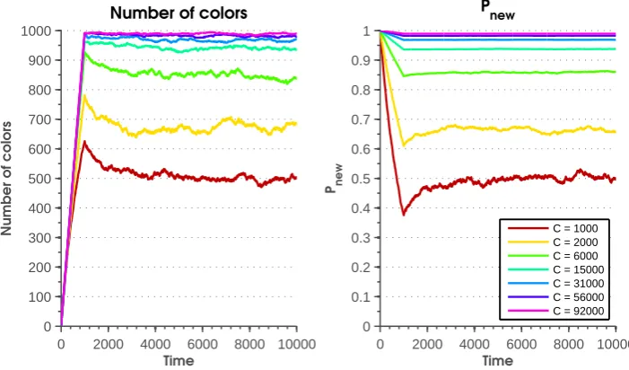
0 0.5 1 1.5 2 2.5

x 104 0

1000 2000 3000 4000 5000 6000 7000 8000 9000 10000

Time

Number of colors

0 0.5 1 1.5 2 2.5

x 104 0

0.1 0.2 0.3 0.4 0.5 0.6 0.7 0.8 0.9 1

Time Pnew

P

new

[image:32.595.120.474.96.321.2]

K = 1000 K = 2000 K = 3000 K = 4000 K = 5000 K = 6000 K = 7000 K = 8000 K = 9000 K = 10000

Figure 5.1:The number of colors in the online structure (left) and the probability to draw a ball from the source that has a color that is not present in the online structure,Pnew, (right) as a function of the time. The probability to draw

a color from the source corresponds to a uniform distribution.

(33)

0 2 4 6 8 10

x 104 0

5000 10000

Time

N(0,t)

0 2 4 6 8 10

x 104 0

5000

Time

N(1,t)

0 2 4 6 8 10

x 104 0

1000 2000

Time

N(2,t)

0 2 4 6 8 10

x 104 0

500 1000

Time

N(3,t)

0 2 4 6 8 10

x 104 0

500

Time

N(4,t)

0 2 4 6 8 10

x 104 0

200

Time

N(5,t)

K=10000

Figure 5.2:The number of queues in the online structure with lengthi,i= 0,1,2,3,4,5as a function of the timet. C=Kand the probability to draw a color from the source corresponds to a uniform distribution.

Note thatN(0, t)is decreasing in the beginning, this is caused by the fact that all the positions in the online structure are empty att= 0. For the same reason in the plots forN(i, t),i= 1, ...,5the number of colors in the queue with lengthiis increasing.

5.1.2 C Colors

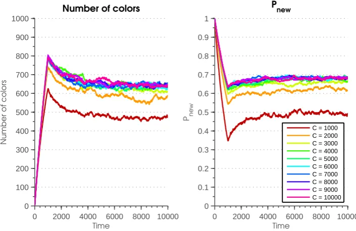
Also in case there is a total number ofCcolors in the game, it turns out that the numerical results indeed correspond to the obtained analytical results.

[image:33.595.121.472.502.708.2]

Variation of the total number of colors

Figure 5.3 presents the numerical results using a fixed value ofKand different values forC.

0 2000 4000 6000 8000 10000 0

100 200 300 400 500 600 700 800 900 1000

Time

Number of colors

0 2000 4000 6000 8000 10000 0

0.1 0.2 0.3 0.4 0.5 0.6 0.7 0.8 0.9 1

Time

P new

P

new

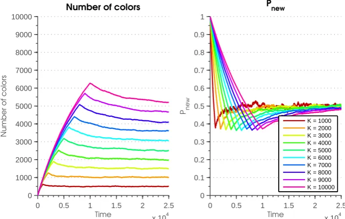
C = 1000 C = 2000 C = 6000 C = 15000 C = 31000 C = 56000 C = 92000

(34)

The figure shows that ifCincreases, whileKremains the same,Pnewtends to1. This is in accordance

with the analytical results that are obtained in Section 4.2, as bothPnewand the number of colors in the

online structure are increasing inC. Furthermore it has been shown in Section 4.2 that ifC tends to infinity thatPnewtends to1and the number of colors in the online structure tends toK. Note that when

C =Kthe results are the same as for the case that there wereKcolors in the game, see Figure 5.1. The expected number of colors att=K also corresponds with the analytical result and asCtends to infinity, the expected number of colors at timeKgoes toK.

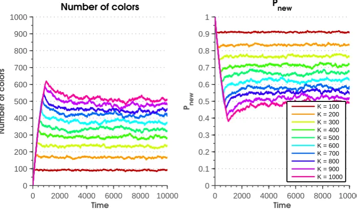
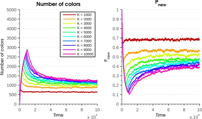
Variation of the number of positions in the online structure

Varying the number of positionsK, when the probability vectorpcorresponds to a uniform distribution, is presented in Figure 5.4. Also this figure is in accordance to the analytical resuls: if C >> K the probability to draw a ball from the source with a color that is not present in the online structure tends to

1.

0 2000 4000 6000 8000 10000 0

100 200 300 400 500 600 700 800 900 1000

Time

Number of colors

0 2000 4000 6000 8000 10000 0

0.1 0.2 0.3 0.4 0.5 0.6 0.7 0.8 0.9 1

Time

P new

P

new

[image:34.595.123.472.272.477.2]

K = 100 K = 200 K = 300 K = 400 K = 500 K = 600 K = 700 K = 800 K = 900 K = 1000

Figure 5.4:The number of colors in the online structure (left) and the probability to draw a ball from the source that has a color that is not present in the online structure,Pnew, (right) as a function of the time for different values of K.C= 1000and the probability to draw a color from the source corresponds to a uniform distribution.

The analytical results say that when, for example,K = 100 andC = 1000the number of colors in the online structure is expected to be91in stationarity andPnewapproximates91%. With these parameters

the expected number of colors in the online structure at timeK is95. Figure 5.4 suggests that this is indeed the case.

5.2 Exponential Distribution

In this subsection the probability vectorpcorresponds to an exponential distribution with meanλ. Since it is a discrete version of the exponential distribution this comes down to a geometric distribution with success probability1−e−λ1.

Variation of the total number of colors

(35)

0 2000 4000 6000 8000 10000 0

100 200 300 400 500 600 700 800 900 1000

Time

Number of colors

0 2000 4000 6000 8000 10000 0

0.1 0.2 0.3 0.4 0.5 0.6 0.7 0.8 0.9 1

Time P new

P

new

[image:35.595.120.473.95.324.2]

C = 1000 C = 2000 C = 3000 C = 4000 C = 5000 C = 6000 C = 7000 C = 8000 C = 9000 C = 10000

Figure 5.5:The number of colors in the online structure (left) and the probability to draw a ball from the source that has a color that is not present in the online structure,Pnew, (right) as a function of the time for different values ofC. K= 1000and the probability to draw a color from the source corresponds to an exponential distribution with mean λ= 1000.

In case thatC =λ, Figure 5.5 shows thatPnewis about 1₂ and that the number of colors in the online

structure is approximately K

2. This was also the case for the uniform distribution if C = K. The cumulative distribution function for the uniform distribution is linear in C. The cumulative distribution function for the exponential distribution is:

F(c, λ) = 1−e

−c λ

1−e−Cλ

,

wherec = 1, ..., C is the color. The normalization is applied because the sum of the elements in the probability vector pshould be 1. It turns out that in case C = λ the uniform distribution is a good approximation for the exponential distribution. This is explained below. Note that when C = λ, the cumulative distribution function is

F(c, λ) = 1−e

−c λ

1−e−1,

Now letg(c)be the difference betweenF(c, λ) and _λc, the cumulative distribution function of the uniform distribution. So,

g(c) = 1−e

−c λ

1−e−1 − c λ, g0(c) = 1

λ

_e−c

λ

1−e−1 −1

.

Note that the functiong(c)is a concave function. The derivative is a decreasing function, becausee−c λ

is a decreasing function and 1−e−1 _{is just a constant. At} _c _{= 0}_, _g0₍_c_{) =} 1

e−1 1

λ > 0 and at c = C,

g0(c) = 2_e₋−₁e_λ1 <0 and it follows thatg(c)is a concave function and the extreme value is a maximum. Solving the equationg0(c) = 0yields:

1

λ

_e−c

λ

1−e−1 −1

= 0,

e−λc = 1−e−1,

(36)

and it follows that the top of the concave function is atc=−λln(1−e−1). The function value at this point is 1

e−1+ ln(1−e

−1_{) = 0}_.₁₂_{. This means that the difference between the uniform cumulative distribution} function and the exponential cumulative distribution function is at most0.12and this could explain why the exponential distribution forpin caseC=λgives similar results as the uniform distribution forp. In the caseC6=λand whenCgoes to infinity, the cumulative distribution function reduces to

F(c, λ) = 1−e−λc.

Because of the discrete exponential distribution the probability that a ball has colorc, wherec= 1, ..., C, is the following:

P(color=c) = e−λ1(c−1)−_e−λ1c_, = e−λ1(c−1)(1−e−

1

λ). (5.1)

Note that there will be convergence of the number of colors in the online structure from a certain point onwards whenCgoes to∞, because the colors at the tail of the distribution are very unlikely to retrieve from the source. Figure 5.5 indeed illustrates this behavior and it means thatPnew is independent of

the total number of colorsC. The convergence can also be seen in the expected number of colors at timeK. With a constant meanλ= 1000and withK = 1000the expected number of colors at timeK converges to approximately796.

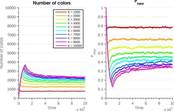
[image:36.595.121.475.415.624.2]

Variation of the number of positions in the online structure

Figure 5.6 shows what happens when the number of positions in the online structure,K, is changing, while the total number of colorsCand the mean of the exponential distributionλare fixed.

0 2 4 6 8 10

x 104 0

500 1000 1500 2000 2500 3000 3500 4000 4500 5000

Time

Number of colors

0 2 4 6 8 10

x 104 0

0.1 0.2 0.3 0.4 0.5 0.6 0.7 0.8 0.9 1

Time

P new

P

new

K = 1000 K = 2000 K = 3000 K = 4000 K = 5000 K = 6000 K = 7000 K = 8000 K = 9000 K = 10000

Figure 5.6:The number of colors in the online structure (left) and the probability to draw a ball from the source that has a color that is not present in the online structure,Pnew, (right) as a function of the time for different values of K.C= 100000and the probability to draw a color from the source corresponds to an exponentail distribution with meanλ= 1000.

(37)

Variation of the meanλ

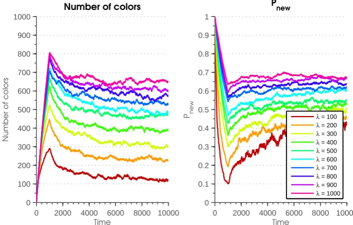
The last figure for the probability vector that corresponds to an exponential distribution shows a variation ofλ, the mean of the exponential distribution.

0 2000 4000 6000 8000 10000 0

100 200 300 400 500 600 700 800 900 1000

Time

Number of colors

0 2000 4000 6000 8000 10000 0

0.1 0.2 0.3 0.4 0.5 0.6 0.7 0.8 0.9 1

Time P new

P

new

λ = 100

λ = 200

λ = 300

λ = 400

λ = 500

λ = 600

λ = 700

λ = 800

λ = 900

[image:37.595.118.471.151.376.2]

λ = 1000

Figure 5.7: The number of colors in the online structure (left) and the probability to draw a ball from the source that has a color that is not present in the online structure,Pnew, (right) as a function of the time for different values

ofλ. C = 100000,K = 1000and the probability to draw a color from the source corresponds to an exponential distribution with meanλ.

When λincreases, the figures shows that the number of colors in the online structure increases, as well asPnew. Remember the formula of the probability that a ball is of colorc, see (5.1). WhenCis a

constant andλis a variable then this is an increasing function, as the derivative shows: dP(color=c)

dλ =e

−c λ

h

c(eλ1 −1)−e 1 λ

i

.

Optimization of the BUbiNG web craler