University of Twente
School of Management and Governance Master Thesis
Predicting the sales figures of TVs using data from Google Trends
Programme: MSc Business Administration
Student name: Lars Phillip Lehmann
Student number: s1312464
E-Mail: [email protected]
Supervisors: Dr. A.B.J.M. Wijnhoven
Dr. H.G. van der Kaap
Date: 16. August 2016
Abstract:
2
Content
1 INTRODUCTION ... 3
2 THEORETICAL FRAMEWORK ... 6
2.1LITERATURE SEARCH STRATEGY ... 6
2.2PREDICTION... 6
2.2.1 Concept ... 6
2.2.2 Types of prediction ... 8
2.2.3 Predictions in social media research ...11
2.3METHODS ... 11
2.4PRECISION AND VALIDITY ... 15
2.4.1 Precision ...15
2.4.2 Validity ...16
2.5RELIABILITY OF DATA AND PLATFORMS ... 19
2.6TIME LAG ... 22
3 METHOD ... 25
3.1RESEARCH DESIGN ... 25
3.2DATA COLLECTION ... 27
3.3DATA ANALYSES... 28
4 RESULTS ... 31
5 DISCUSSION AND CONCLUSION ... 37
5.1KEY FINDINGS... 37
5.2DISCUSSION ... 38
5.3LIMITATIONS & FUTURE RESEARCH ... 39
5.5PRACTICAL IMPLICATIONS ... 39
6. GERMAN TRANSLATION ... 41
REFERENCES ... 44
APPENDIX ... 47
APPENDIX A:KEYWORDS ... 47
3
1 Introduction
Previous research suggests that effective forecasting management may lead to improved business performance (Moon, Mentzer, & Smith, 2003). Data from traditional surveys is not always available fast, and only with high level of aggregation and a small set of variables, making identification of trends difficult (Wu & Brynjolfsson, 2009). During Web 1.0, the first natural language processing tools emerged, but with the explosion of Web 2.0 platforms, opinion mining techniques became more urgent and useful due to the rapidly increasing amount of content on the internet (Pang & Lee, 2008). Personal weblogs and online review sites delivered new opportunities for analysts to gather and analyse individuals’ opinions. Multiple forms of reviews emerged; the sentiment measures from social media sites and blogs, as well as the star ratings for product review sites like CNET, and finally review reports on product review sites like Amazon. However not all of these sources can be used equally, because users’ star ratings are often more positive than sentiment classifications (Wijnhoven & Bloemen, 2014). Furthermore, due to the interest of businesses to promote their own products, review spam is a problem on e-commerce sites (Pieper, 2016).
4
The goal of this research is to develop reliable predictions for electronic consumables for a company, using information from search queries on Google. Currently, the company, a retailer for electronic goods, uses historical data to forecast sales volumes one year in advance. However the forecasts are for income from sales and not for the number of units to be sold. So there is a need for a more accurate forecasting method in order to facilitate inventory planning. Forecasting sales numbers can help retailers to better plan their inventory, since customer demand is known to some degree. This can save money since inventory can be kept smaller and managed more efficiently. Also customer satisfaction can rise or stay at high levels if the customer is always able to get what he is looking for at a retailer. TVs are rather big and take up a lot of inventory space, so planning the inventory accordingly is crucial. Thus, the research question that leads this research is: ‘How to predict the sales numbers of TVs?’
5
This thesis aims to make a contribution to practice by helping companies in the decision making process of inventory planning by enhanced sales prediction. The intended outcome is a method that can predict future sales figures as precise as possible. Due to the limitations of this project, only one data source will be used, either Google Trends or Twitter. The decision will be based on a comparison between the reliability and validity of the two data sources. The focus of this thesis is on electronic consumables, more specifically TVs. Thus, the research might not be applicable to all goods at every retailer but it could be tested in future research.
6
2 Theoretical Framework
2.1 Literature search strategy
There has been a lot of research aimed at identifying the predictive power of Google Trends and Twitter. The search for ‘Google Trends prediction’ delivers approximately 842,000 results on Google Scholar and 4,650 results on ScienceDirect respectively. Furthermore, the search for ‘Twitter prediction’ delivers 2,380,000 results on Google Scholar and 1,930 results on ScienceDirect. The scientific journals International Journal of Forecasting and MIS Quarterly often publish articles about prediction and forecasting using social media content. Therefore, these search engines and journals serve as useful sources for a literature search for this study. Data from Twitter or Google Trends was used most often in these articles, since data from these sources are publicly available.
The research question, ‘How to predict the sales numbers of TVs?’, and the following five subquestions serve as a guideline for the literature search. (1) What is a prediction? (2) What are the existing methods for predicting sales of a specific product? (3) What is the precision and validity of the measurement? (4) What is the reliability of the data? (5) What is the time lag between the variables?
2.2 Prediction
2.2.1 Concept
7
Forecasting is the use of information for the identification of a single future event that takes place with certainty (Kusunose & Mahmood, 2016). For example it can be forecasted if it is going to rain tomorrow based on past observations with similar climate conditions. Time-series analyses to predict future observations are generally called forecasts in literature (Asur & Huberman, 2010). Therefore, forecasting is a subset of predictions. Forecasting of sales includes the analysis of human behaviour, which can be difficult given the huge amount of different factors that influence individuals. In order to facilitate working with many individuals’ values, instantiation can be used to categorise individuals. The pragmatic value is to help avoiding variation, a source of nuisance caused by individual differences (Moore, 2015). This means for buying behaviour to classify customers based by the content of their tweets instead of demographics or other information and create profiles. However, it is possible to acquire simple demographics like gender and age rather accurately from usernames but it is not always useful (Wijnhoven & Bloemen, 2014).
8
makes the theory in forecasting and prediction important, which is used to explain the relationship.
2.2.2 Types of prediction
Predictions say what is and what will happen, but it is not necessarily explained why (Gregor, 2006). According to Gregor (2006), also a prediction with an explanation is possible. In predictions without an explanation, theorists focus on predicting patterns with testable propositions but lack causal explanations. Predictions with an explanation can tell what is, how, why, when, where, and what will be. Theorists focus on predictions with testable propositions as well as causal explanations (Gregor, 2006). According to Shmueli (2010) the difference between explaining and predicting lies in the fact that the data measured are not exact representations of the underlying constructs. Due to the operationalisation of constructs and theories into measurable data and models a disparity between an explanation of a phenomenon and a prediction is created. Further, explanations include the use of explanatory modelling and statistical models for testing causal explanations. Predictive modelling involves applying a statistical model to data in order to predict future observations, often without a causal explanation (Shmueli, 2010). As already mentioned, searching for a TV model probably does not directly lead to a purchase, therefore in this case a prediction without an explanation will be used.
There are various categories, approaches, and methods for predicting, for example the qualitative approach, the quantitative approach, the average approach, the naïve approach, causal forecasting methods, and the self-fulfilling prophecy.
9
social media, is one method of quantitative prediction. It has often been used via social media analytics for solving problems and predicting various outcomes, e.g. presidential elections or human behaviour (Surowiecki, 2005). Three conditions have to be met in order to form a “wise crowd”. First, each person should have some private information, to ensure diversity. Second, independence of individuals is also important, so the opinions of individuals should not be influenced by others. Finally, private judgements should be turned into a collective decision (Surowiecki, 2005). This research will focus on quantitative methods for predictions because big data will be used instead of experts’ judgement.
Average approaches predict that future values are equal to the mean of their respective past data (Hyndman & Athanasopoulos, 2014). An example for the average approach is the use of the average of sales of a TV model for January to June in order to predict the monthly sales of a TV model for July to December. However, this approach might not be the most useful in this case, since TV sales have seasonality and the life cycle of a model is rather short. TV sales have a peak in autumn but they tend to stagnate during the summer months. The maximum lifespan of a TV model in the sample is 22 months, so not too much historical data can be gathered. Using the average of two different years, e.g. comparing the average sales of 2013 to predict sales for 2014 might thus not be accurate enough to predict specific models. Therefore this approach will not be used in this case but it is worth mentioning.
10
Causal prediction methods, also called econometric forecasting methods try to identify influencing factors to the variable that is being predicted (Nahmias, 2009). For example, including the influence of an event, like the football world cup in the forecast of TV sales. Typically this method is not used for prediction but rather as part of a prediction model in order to identify influencing variables. Therefore this method can be used to explain fluctuations in the data, but it can be difficult to identify all factors that are influencing a forecast.
11
2.2.3 Predictions in social media research
Predictions in social media research try to make a statement about a real-life event based on activity on social media. Social media can be related to various events, for example whether sales numbers for a product will increase or decrease. The hypothesis for predictions about sales numbers based on social media is basically that if a product receives more attention in social media, more people will see it and thus more people will finally buy the product, so sales will increase, or vice versa. The last example of a self-fulfilling prophecy is an example for the reason why the hypothesis might be rejected, since more ‘bad’ attention on social media can lead to a decrease in sales numbers. Therefore sentiment mining can be used to determine whether the content of a tweet is positive or negative and so it can be compared if there are more positive or negative tweets about a product. However a lot of positive sentiment might come from the company selling the product, which could distort the data. Also spam messages are still a problem in social network, with around 6% of all tweets on Twitter being spam. Spam messages contain almost exclusively promotional content, even though the links in the tweets redirect to malicious sites (Chen et al., 2016). Therefore, the prediction methods and the variables might have some reliability and validity issues. Additionally social media can also provide information about the viral spread of messages, the reach and strength of posts, as well as trends. The spread, reach, and strength of promotional tweets for a specific product could be able to predict demand of the product but it is not clear if this is sufficient for an accurate prediction. One difference between predictions based on Google Trends and Twitter is that the value of the predictive capability of Twitter lies in the persuasive communication of some people, while the predictive capability of Google lies in the interest in something by many people.
Moreover, the reliability of the collected data and the method of collecting data are important to the overall reliability of the result. The issues of reliability and validity of methods and data are discussed in the next sections.
2.3 Methods
12
gather and analyse individual’s opinions (Pang & Lee, 2008). With traditional research methods, data is not available as fast as with social media or search engines. These new methods make prediction of future trends easier and more accurate (Wu & Brynjolfsson, 2009). Information technologies and computational methods have been developed to deal with opinions directly and predict future trends, sales or other relevant data. When social media gained popularity, people began to share their content there and built up social networks.
There are various search engines and social media platforms available that can be used to retrieve trend data. Web-search engines that can be used are among others Google, Yahoo!, and Bing. The most popular social media websites are Twitter and Facebook with 320 million and more than 1.6 billion monthly active users respectively (Facebook, 2016; Twitter, 2016). Monthly active users are defined as individuals that log into their social media account at least once a month. Data from Google is easily available via their service Google Trends, a successor of Google Insights for Search, which was used in some studies. Vosen and Schmidt (2011) show that Google Insights for Search can predict private consumption more accurately than the traditional survey-based predictions. However, since Google Insights for Search is not available anymore, Google Trends can be used to gather search volumes on a topic. Choi and Varian (2012) used Google Trends for predictions in various categories. Their model that included Google Trends was able to outperform the model that only uses traditional approaches, e.g. expert judgements. Wu and Brynjolfsson (2009) were able to predict future quantities and prices in the housing market by using data from Google. The authors state that the approach can also be applied to other markets.
13
The information created daily on the various social media sites and search engines can be used to gather opinions in higher quantities compared to previous methods. Several studies have shown the effectiveness of social media as a method for predicting real-world outcomes (Ahmed et al., 2016; Asur & Huberman, 2010; Bollen et al., 2011; Burnap et al., 2016; Lassen et al., 2014). Some prediction models even receive more accurate results than an information market, e.g. Hollywood Stock Exchange for movie box-office revenue predictions. Asur and Huberman (2010) collected data from Twitter referring to movie releases during a specific time period, in order to predict box-office revenues for movies in its opening weekend. They analysed the number of tweets referring to a particular movie per hour (tweet rate) and the box-office gross and found a significant positive correlation (R=0.9, adjusted R-square=0.8). Based on this, a model using least squares was developed. It turned out that a model using linear regression of time-series values of the tweet-rate for seven days before release together with the positive-negative ratio was most reliable for predicting the box office gross at the end of the week after release (adjusted R-square 0.94).
14
values. In future research, this approach can be tested for other stock markets in specific regions or other objects someone aims to predict.
Risius et al. (2015) also try to link movements in the stock market to emotions derived from social media. They developed a dictionary for the analysis of seven emotions. The seven emotions are: affection, happiness, satisfaction, fear, anger, depression, and contempt. They analysed the sentiments of Twitter messages about specific stock listed companies, not general Twitter messages like Bollen et al. (2011) did in their research. Risius et al. (2015) categorised the emotions into positive and negative emotions but found that a more differentiated sentiment was needed. Overall, when comparing positive and negative valence, they found that only the average negative emotionality strength, i.e. fear, anger, depression, and contempt, has a significant connection with company-specific stock price movements. It can be assumed that this is a bias caused by a larger dictionary for negative than for positive emotions. However, an increase in the emotions ‘depression’ and ‘happiness’ is negatively correlated with company-specific stock prices (Risius et al., 2015). The research was limited to a specific region, since only companies on the New York Stock Exchange were studied and the tweets analysed were in English. However the method of this research could also be used for prediction and forecasting in other areas.
Another study using sentiment data from Twitter was conducted by Hill, Benton, and Bulte (2013). They showed that Twitter data can be useful for deciding when to use social network-based or collaborative filtering methods for making better recommendations. The social network-based system makes recommendations based on a user’s local follower network, while the collaborative filtering-based method compared users based on their interests and the brands they follow. The social network-based system works for a small number of recommendations, and the collaborative filtering-based method works better for higher numbers. This research shows that social media can predict interests of individuals based on their profiles. Further research can analyse whether this interest can lead to an increase in sales for a specific product.
15
precision, validity, and reliability. In the next section it will also be decided whether to use Google Trends or Twitter Analytics for predictions.
2.4 Precision and Validity
2.4.1 Precision
Measurements can be made with varying degrees of precision, for example it is more precise to have exact sales numbers for a time period, i.e. ‘172 of model XY in June 2013’, rather than rough estimates, i.e. ‘between 100 and 200 of model XY in June 2013’. Precision is concerned with the fineness of distinctions made between the attributes that compose a variable (Babbie, 2013). Precision can be achieved by observing multiple measurements under the same condition. In order to increase the precision of sales numbers, the data of various stores for the same TV models are needed.
16
Precision of social media analytics include the date when a tweet was published and the exact amount of positive, negative, and neutral sentiments. Depending on the tool used, the precision of the gathered data can differ, since some tools do not incorporate all tweets published. However most tools include the exact date a post was published, even stating the exact minute of publication. This makes Twitter very precise concerning the date of a tweet. The specifications for positive, negative, and neutral sentiments differ for each tool, and they are not always classified correctly (Serrano-Guerrero, Olivas, Romero, & Herrera-Viedma, 2015). Therefore the measurement of sentiment might be precise but has the problem of construct validity.
2.4.2 Validity
Validity is often a concern for predictions based on Google Trends and social media, since samples can be biased (Wijnhoven & Bloemen, 2014). Generally, validity is defined as the extent to which an empirical measure completely reflects the actual meaning of the particular concept (Babbie, 2013). Validity can be distinguished into many types, the following five types are chosen for this research, since they are expected to cover most of the subject; face validity, criterion-related validity, construct validity, content validity, and inferential validity.
Face validity requires the indicator to be a reasonable measure of the variable (Babbie, 2013). In this case the question is whether Google Trends and Twitter data can be considered to be an adequate indicator for the amount of interest in a certain product. According to marketing literature, individuals search for information about a product before the purchase (Hassan et al., 2014; Kotler, 2000). This information search can be done online, so that the amount of search queries on Google can serve as an indicator for the interest in a product. On Twitter, opinion leader offer advice about products and the reach of these tweets can indicate the interest in a product. Additionally, previous studies were able to successfully make predictions using data from Google Trends and Twitter, so it can be assumed that the requirements of face validity are met. For the sales data, the monthly sales numbers are expected to accurately predict the overall amount of sales of the same products, so face validity is achieved.
17
Board tests is shown in their ability to predict the success of students in college (Babbie, 2013). For this study, it implies that the individuals’ behaviour measured by Google Trends data and Twitter Analytics data can actually be an indicator for the sales of TVs. It is not expected that search queries directly lead to sales, so there is no causality between the variables. Even though there is no direct causal relation between these variables, recent research has proven that either social media or search engine data can predict box-office income (Asur & Huberman, 2010) the stock market (Bollen et al., 2011), sales numbers of smartphones (Lassen et al., 2014), and housing prices (Wu & Brynjolfsson, 2009). Therefore it can be assumed that Google Trends data and Twitter Analytics data could predict sales numbers for TVs as well.
Construct validity can be defined as the degree to which the data covers the underlying construct. The construct validity of sentiment analysis based on Twitter data is dependent on the tool used. Validity can be measured by the precision of the tools classifying sentiments. It can be distinguished between negative, neutral, and positive precision, where negative precision is the relative amount of correctly classified negative sentiments in a tweet as negative. Neutral precision is the relative amount of correctly classified neutral statements as neutral in tweets, and positive precision is the relative amount of positive sentiments in tweets that were classified as positive. Serrano-Guerrero et al. (2015) compared the precision of classifications made by 15 Twitter Analytic tools and found that the precision of these tools ranges from 51% to 88.1%. So, validity heavily depends on the tool used but complete construct validity does not seem to be possible, since the data cannot cover the full construct. Google incorporates a percentage of all searches in Google Trends only, instead of all search queries that are performed on Google (Google, 2016d). Construct validity for the sales data might be a problem, because the sales numbers are from one retail chain only. The sales could have been different for other retailers, especially due to special offers from retailers. The requirements of construct validity can thus not be met by the data.
18
a customer to buy than the number of searches on Google and sentiments of tweets on Twitter, however social media data is rather easy to acquire in high volumes compared to e.g. traditional surveys. Furthermore Google Trends might not measure a representative sample of the population, since young age, high education, and high income have a positive influence on Internet usage (Perrin & Duggan, 2015). Another issue of content validity is whether the chosen search terms represent the issue being measured. Misspellings, spelling variations, synonyms, singular or plural versions are not included in Google Trends, because they can all change the actual meaning of a term (Google, 2016c). Furthermore in Google Trends it can be selected to only show results from the category ‘consumer electronics’, so that for example TV shows are excluded from the results. This increases the content validity of Google Trends searches.
19
2.5 Reliability of data and platforms
Reliability of a method can be achieved, if the same technique applied to the same object yields the same result each time (Babbie, 2013). Thus, the method has to be performed multiple times, e.g. for a control sample from the overall sample, with the same result to be considered reliable. In order to increase reliability, several sources of data can be used. However using both Twitter and Google Trends data takes a lot of time and the timeframe for this research is limited so only the method that is expected to be more useful will be used. The usefulness of each platform is based on the validity and reliability for the research goal. It has been shown in the previous section that there is almost no difference in the validity of the data.
20
of the studies that show the Type I errors, while the file drawers are filled with the 95% of the studies that show non-significant results and will never be published (Rosenthal, 1979). The Type I error refers to the incorrect rejection of a true hypothesis, due to researchers getting significant results that the null hypothesis false. For example the null hypothesis ‘social media has no predictive power’ can seem to be false, even though it could actually be true. Even though there are many articles using the predictive power of Twitter analysis and Google Trends, we do not know how many efforts to find these relationships have failed (Couper, 2013). Hence, it might be possible that only studies that support hypotheses that are in favour of social media prediction are reported in journals. Finally, according to past events, social media services may be popular for a rather limited time, e.g. Myspace was once the most popular social media site but is barely used anymore today. Social media platforms fluctuate in user size over the years, which makes long-term studies using social media more difficult (Couper, 2013).
Search engines gather data from users by their search behaviour. Google also gathers demographic data from the user when they use Google’s services, more specifically, the approximate location. Information that is shared publicly by Google is not personally identifiable, so it is not possible to identify the purchasing process for individuals based on the data (Google, 2016b). Google Trends data is collected from a percentage of Google web searches and used to identify the number of searches over a certain time period. Searches that are made by very few people as well as duplicate searches by the same person over a short period of time are not included in Google Trends, so that distortions in and manipulation of the data is less likely (Google, 2016c). Specific words and spellings that change the meaning of the searched phrase can also be automatically excluded by choosing a category, if necessary. Therefore Google Trends searches can be rather flexible and conditionally more precise, if the right search terms are chosen by the researcher.
21
Google Trends contains all the data needed, i.e. monthly search volume and location, and is easily available, but for Twitter the data has to be gathered via a third party tool, including content, date, and location of the tweet, as well as demographic data, if available. Then the text has to be classified for sentiments and then further analysed. Tools that are able to perform these tasks are social mention, coosto, AlchemyAPI, sproutsocial, just to name a few. Social mention is a free tool for real-time search, which can measure the strength, sentiment, and reach of tweets. However, it does not provide historic data that is older than one month; hence the data needed cannot be gathered. Also validity is not given, since only one point or few points in time are measured, instead of a time series. Coosto can provide older data and analyse opinions, but is not available for free. AlchemyAPI is an API that can be used the build applications for any purpose but it requires prior programming knowledge and is also not free. Sproutsocial is able to monitor keywords and locations over time, but is also not available for free. The analytics tools are meant for organisations to track their visibility and reach on social media, so they are not available for free. Furthermore, most work slightly different, for example in the way they analyse sentiment, which tweets they include, and the timeframe they analyse. Also, sentiment analysis is still biased to some degree, since it focuses on the choice of positive and negative words and often does not understand sarcasm, which shifts the meaning of something to the opposite (González-Ibáñez, Muresan, & Wacholder, 2011). Also in the case of sentences like ‘A is better than B’ or ‘B is better than A’, the same words are used, but the objects are rated differently.
Even though sentiment analysis has shown to be useful in some cases, it is not useful when predicting car sales because there is no significant correlation between sentiments and car sales (Plant, 2016). Social media sentiments have little to no predictive power in the case of car sales, which sets clear limits to the field of sentiment analysis (Plant, 2016). This suggests that Twitter Analytics might be more useful in other areas than sales predictions. Since Google Trends is easier to use, has more precise demographics, and does not rely on imperfect sentiment analysis, it might be an overall better and easier choice for predicting sales numbers in this case. Therefore this research will only use Google Trends data to predict the sales numbers of TVs.
22
between the increase of interest about TVs on Google Trends and the increase in TV sales. This time lag is discussed in more detail in the next section.
2.6 Time Lag
The time lag is defined as the period of time between the occurrence in the data and the actual predicted event happening. For example the change in Google Trends data might be occurring in week 15, but the same change in sales can be observed in week 18, so that the correlation increases when introducing a time lag of three weeks. In practice it is expected that a change in sales is happening some time after a change in Google Trends data. It is not yet clear how long the time lag in the case of TV sales will be; it might differ for each product category and price range.
Choi and Varian (2012) use data from Google Trends to predict the present, by using Google Trends data for a certain month to predict sales for the same month. However, in order to predict the future, instead of the present a time lag should be considered in the prediction model. Asur and Huberman (2010) use a time lag of one week for the prediction of box office revenues based on tweets. In other research the time lag for smartphones was already measured, i.e. the strongest correlation between tweets containing the keyword ‘iPhone’ and actual purchases of iPhones was found using a time lag of 20 days (Lassen et al., 2014).
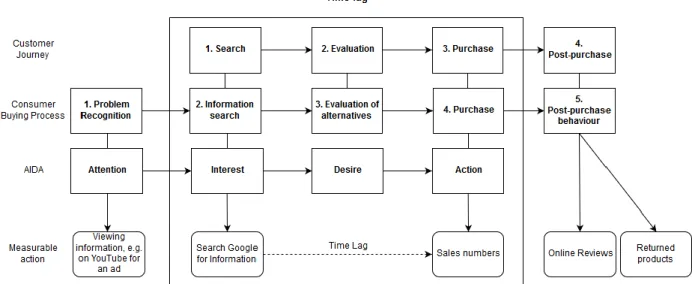
There are different models from marketing that can explain the time lag, for example the five stages of the buying process by Kotler (2000). The first stage involves the customer recognising a problem, followed by the information search. Then the evaluation of alternatives takes place and finally the customer decides to purchase the product. The fifth stage consists of the post-purchase behaviour. The data on Google Trends is generated during the second stage, if the customer searches for information via Google for the product. The sales data is generated at some point during the fourth stage. Thus, the time lag occurs between these stages, namely the information search and purchase decision.
23
Finally the post-purchase phase can occur, where the customer can give feedback about the product, e.g. by an online rating, return a product, or plan the next purchase.
24
review site, and the number of returned products could serve as measurable actions for this phase, even though they do not cover the full concept. The last phase is not necessary for this research, since the focus will be phases from interest to action. The relations between the three models and the measurable actions are shown in Figure 1.
In prediction theory using Google Trends, the time lag is the time passing between the interest and the action phase. In the data a time lag is expected between the search query and the final sales numbers. It should be noted that not all consumers who show initial interest in a product by searching it on Google will also desire or even buy the product. The post-purchase activities are also optional. In the next section the data collection method is elaborated based on the theories.
25
3 Method
3.1 Research design
For the quantitative analysis, sales numbers for categories of TV models are compared with data from Google Trends. Google Trends analyses the number of searches for a specific term and gives a number between 0 and 100 as an output. Thus the independent variable will be the relative search volumes. The relative number provided by Google Trends can be summarised as trends. The independent variable, trends, is expected to have a positive influence on the dependent variable. In this case the dependent variable will be the number of sales of a specific TV. Due to the rather high price, the purchase decision might be less intuitive for customers, which are expected to inform themselves about a TV model before the actual purchase. The category TV is supposed to serve as an example for other goods in retail, for which this study is supposed to be repeatable.
H1: The number of TV sales increases when the number of searches on Google for the related TV model increases.
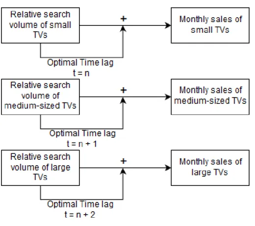
Generally for TVs, a time lag is expected, since they are a rather expensive good so that customers generally might evaluate the purchase decision of a new TV for a longer time than for less expensive goods. So as a third variable, the optimal time lag between tipping points will be introduced. The time lag might differ depending on the price of a specific TV, as it could be longer for more expensive TVs and shorter for cheaper TVs. This assumption is based on previous research suggesting lower prices have a direct positive influence on purchase intent (Somervuori & Ravaja, 2013). Time lag is defined as the time between the customers’ initial interest in a product and the actual purchase of the product. Accounting for a time lag can be important for all product types with higher price ranges. Introducing a time lag is expected to either weaken or strengthen the relationship between trends and sales. The optimal time lag is at the point of the highest cross-correlation between trends and sales.
26
prediction (sales), the relationship between trends and sales becomes stronger.
Customers are expected to be less likely to search for the exact TV model names, e.g. ‘UE-32 F 5570’ in search engines because they are rather complex and difficult to remember. According to salespersons at the retailer, most customers mainly focus on the size of the screen, the price of the TV, and sometimes the brand, and less on the technical features. Prices tend to fluctuate for the retailer due to special offers and age of the TV model. Hence, a categorisation for different screen sizes could be more stable. Even though in the long term there is a trend towards bigger TV screens, this trend might not affect the analysis, since the time period for analysis is three years only. TVs with larger screens tend to be more expensive than TVs with smaller screens.
H3: The time lag is expected to be longer for TV models with larger screens.
27
3.2 Data Collection
The sales data of TVs are retrieved from a retailer for electronic goods with several stores in Europe. The data was gathered from ten stores with similar sales space (994 m²- 1,350 m²) within two regions in western Germany, namely North-Rhine Westphalia and Lower Saxony. The sales data is collected during the month and the number represents the total amount of TVs sold by the last day of each month. In total 123 different TV models were selected. The product lifecycle, the total time during which a specific TV model is sold, varies. The average is 12.66 months with four months being the lowest and 22 months being the longest lifecycle of a TV model. The data were collected over the time of three years (36 months), namely from January 2013 until December 2015. The timeframe is supposed to be as long as possible in order to reduce variability and increase validity. A longer timeframe is not possible since the retailer introduced new central software for accounting in 2013. Also a longer timeframe might not be necessary since 22 months is the longest period during which a single TV model was sold. The data are entered in a database in SPSS in order to test the data for linear regression. A TwoStep Cluster analysis with a maximum number of four clusters will be performed to categorise the TV models. The analysis creates three clusters that categorise the TV models as large, medium, and small. Large TV models are ≥ 46”, with the maximum in the data being 55”, medium-sized TV models are smaller than 46” and larger than 32”, and small TV models are ≤ 32”, with the minimum in the data being 22”. The first cluster contains of 31 cases, the second of 50, and the third cluster contains of 42 cases.
28
words before or after the chosen keyword, for example in searches for ‘46” TV’, also results for ‘buy 46” Samsung TV’, ‘low priced 46” TV’, or ‘new 46” Panasonic TV’ are included. Therefore, brand can be neglected as a characteristic. Additionally the term ‘TV’ should be included in the keyword for clarification. So, the term ‘TV’ and the size in inch are included in the keyword. The keywords are entered in Google Trends respectively and then filtered for Germany during the time period between January 2013 and December 2015. Additionally, a filter can be applied in Google Trends, so only search terms related to ‘consumer electronics’ are chosen. This way, queries for TV shows or channels, e.g. N24 are excluded, which otherwise would show up in the search for ‘24” TV’, thus increasing content validity. A list of TV models and their respective keywords and clusters is shown in the Appendix. The keywords can be entered in the Google Trends search engine and then downloaded as a .csv file from the Google Trends website. In the file, the search volume is presented per week, from Monday to Sunday; therefore some weeks lie in two different months, which can be a problem since the number of sales is presented per month. However the graph on the Google Trends website can show the relative search volume per month, so these numbers are transferred from the website to SPSS manually. This way it is possible to compare monthly sales numbers with monthly trends. The values Google Trends delivers are relative values, so the months where the keyword is searched for most often is always labelled with 100, which is the maximum.
3.3 Data analyses
29
the P-value is larger than 0.1, the null hypothesis will not be rejected. In order to measure the direction and strength of the relationship between the variables, the correlation coefficient R² is used. R² presents the predictive power of the independent variable.
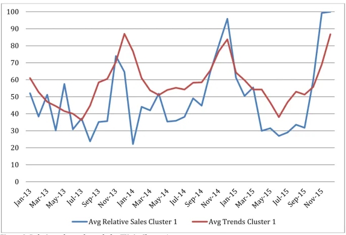
Figure 3 shows a line graph which presents the values of the average of the relative search volumes for the TVs in Cluster 1 on Google Trends and the average of the relative sales of all TVs in Cluster 1 on the Y-Axis. The relative sales numbers were chosen for this graph only since they can be better presented in a line graph next to the trends, which were already relative. For the analysis, the sales data is presented in absolute numbers. On the X-Axis the date is presented per month for 36 months.
Figure 3: Relative sales and trends for TVs in Cluster 1
To test the second hypothesis, the best time lag has to be found. The optimal time lag can be identified by measuring when the correlation coefficient is the highest. It will be tested by measuring the correlation between trends and sales for different time lags. For example the trends curve makes a shift of one month and if the correlation increases compared to the original measure, the time lag is at least one month. This will be tested for one until up to 22 months, since this is the longest life expectancy of a TV model that was measured in this dataset. At the point where the highest correlation between sales
0 10 20 30 40 50 60 70 80 90 100
30
and trends occurs is the best time lag. If the highest correlation between the variables occurs during the original measure, then it can be assumed that there is no time lag. For the analysis, the correlation coefficient, significance, and R-square from the linear regression that was conducted for the test of the first hypothesis are reported. Then a cross-correlation analysis is conducted via SPSS to find the optimal time lag. The time lag is then applied during another linear regression analysis. This analysis is also performed with a 90% confidence interval, so results with a P-value higher than 0.1 lead to a rejection of the null hypothesis. The new R-square value will then be compared to the R-square value of the original measure to check if there are significant improvements of the predictive power. The null hypothesis is that the R-square value will not improve when a time lag is introduced to the relationship. If there is an improvement in the predictive power, then the null hypothesis will be rejected, but if there is no improvement, the null hypothesis will not be rejected.
Finally the third hypothesis expects that the time lag is longer for TV models with larger screens. If the results of the analysis for the second hypothesis do not deliver clear results, this hypothesis will be tested with a t-test. First, all TV models are listed with their size and the corresponding time lag and the median will be used as cut point between large and small TVs. Then an independent samples t-test will be performed to compare the means. A confidence interval of 90% is applied. The null hypothesis states that there is a significant difference between the time lags of larger and smaller TVs.
31
4 Results
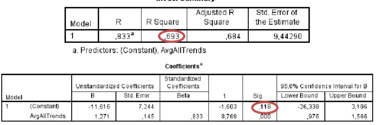
First, a general analysis has been performed with the average value of all sales for all TV models and the average of all trends values over the full time period of 36 months. According to the first hypothesis, the number of TV sales increases when the number of searches on Google related to a specific TV model increases. Therefore the null hypothesis is that there is no relationship between the variables trends and sales. Table 1 shows the results of the analysis with values for R-square and adjusted R-square, but the latter is only necessary when introducing a third variable, so it is not used here. R-square equals 0.693, so there is a positive relationship between the variables trends and sales. The value 0.693 means that approximately 70% of the variance in the sales variable is explained by the trends. The result is significant at a p < 0.01 level, while p < 0.1 would have been sufficient to indicate statistical significance in this case. The standard error of the estimate measures the accuracy of predictions made and it is made up of the sum of the squared errors of prediction. 9.44 is a relatively low value, considering 36 cases with a maximum value of 153.6. This means that the observed value cluster rather closely to the regression in scatterplots, which can be found in Appendix B, Figures 7, 8 and 9.
Table 1: Linear Regression Analysis for sales and trends of all TV models (N = 36)
32
Table 2: Linear Regression Analysis for trends and sales of Cluster 1 Results (N = 36)
For Cluster 2, the medium-sized TVs, the R-square is 0.444, so the relationship is also positive. The result is significant at a p < 0.01 level. The result is similar to the result of the first cluster, but the relationship appears to be slightly weaker.
Table 3: Linear Regression Analysis for Cluster 2 Results (N = 36)
33
Table 4: Linear Regression Analysis for Cluster 3 Results (N = 36)
The second hypothesis states that, when accounting for the time lag between the trends and sales, the relationship between trends and sales becomes stronger. In order to find the optimal time lag, the correlation coefficient between each cluster of trends and sales is measured via cross-correlation. Figure 4 shows the result for cluster 1 in a histogram. The strongest relationship for TVs with the smallest screens is when there is no time lag involved, with an R value of 0.690. Other values are within the confidence interval as well, for example the second highest value is after twelve months, with an R-value of 0.569. However, since the relationship did not become stronger, the null hypothesis that there is no time lag cannot be rejected for this cluster.
Figure 4: Cross-correlation of trends and sales for Cluster 1 (N=36)
34
Cluster 3 does not show improvements of the R-value either; the highest value is 0.817 within the confidence interval. The null hypothesis that there is not time lag cannot be rejected for any cluster. Therefore another linear regression analysis is not necessary. It can be concluded that, if there is a time lag, it has to be shorter than one month.
In order to test if a time lag exists that is shorter than one month, the weekly trends data from the .csv file that could be downloaded from Google Trends is used. The data contains the same keywords and is separated into the same clusters as the original data. The data is presented in weeks, from the beginning of the first week of January 2013, starting at the 06.01.2013, until the end of the last week of December 2015, which ends at 02.01.2016. Furthermore the sales data per week from the ten stores for the same time has been gathered. In total the data from 156 weeks has been gathered. Then the data is separated into the three clusters. Since the number of cases increases from 36 to 156, it is expected that the significance increases as well.
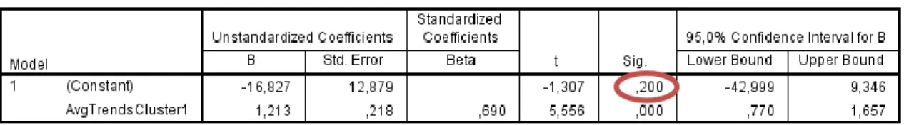
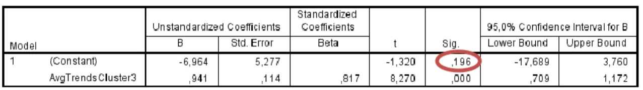
The results of the linear regression with weekly values can be found in Appendix B, Tables 13, 14 and 15. A linear regression analysis of the data indicates a positive relationship for each cluster. Cluster 1 shows an R-square of 0.196, R-square of Cluster 2 equals 0.18, and the R-square of cluster 3 equals 0.338. All results are significant at a p < 0.01 level. Since the time lag is expected to be less than one month, a maximum time lag of eight weeks (≈ 2 months), should be sufficient for the cross-correlation analysis with weekly data.
35
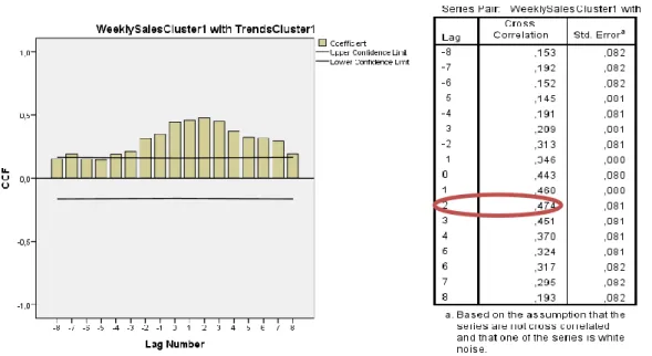
The result for cluster 1 is shown in Figure 5 and the results for cluster 2 and 3 are shown in Figures 13 and 14 in Appendix B. The result of the cross-correlation analysis for cluster 1 shows that the highest correlation occurs with a lag of two weeks (R = 0.474). In cluster 2, the highest correlation occurs with a lag of five weeks (R = 0.549). The highest correlation in cluster 3 occurs when there is no time lag involved (R = 0.582). All values lie within the confidence interval.
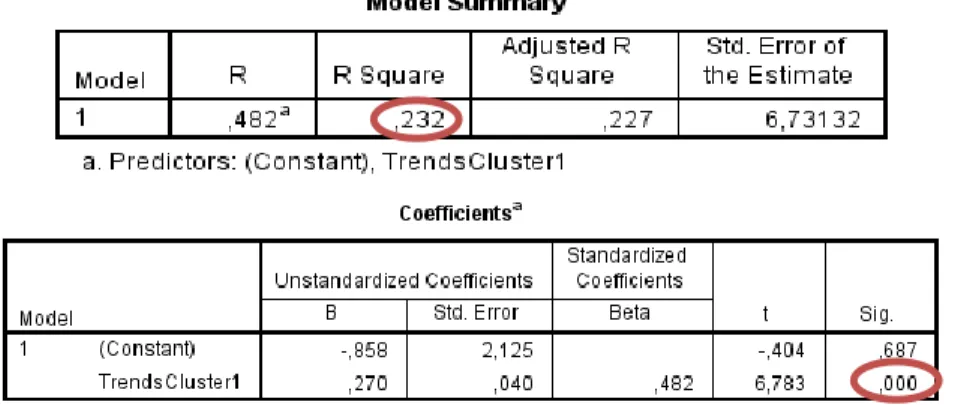
After including the time lag of two weeks, a linear regression analysis of the trends and sales in cluster 1 shows a positive result. The R-square equals 0.232, significant at p < 0.01. Cluster 2 also shows a positive result after introducing the time lag of five weeks to the initial relationship. R-square equals 0.308 and is significant at p < 0.01. The results are summarised in Table 6 and the changes in R-square are calculated. The results show that out of the three chosen categories, two have a time lag between the search on Google Trends and the purchase. With these new results, the null hypothesis that the R-value will not improve when a time lag is introduced to the relationship, is rejected.
Table 5: Linear regression of weekly Trends and Sales for Cluster 1 including time lag of two weeks (N = 156)
Cluster Linear Regression
without time lag Time lag Linear Regression with time lag Changes
R-square Weeks R-square R-square
≤ 32” 0.196 2 0.232 +3.6%
32” < X < 46” 0.175 5 0.308 +13.3%
≥ 46” 0.338 0 0.338 0
Table 6: Changes in R-square after introducing time lag
36
TV models show a time lag of two weeks. It was assumed that the time lag would be longer for TVs with larger screens but it can be seen that the time lag is longer for TVs with smaller screens. Therefore, the time lag is not longer for TVs with larger screens.
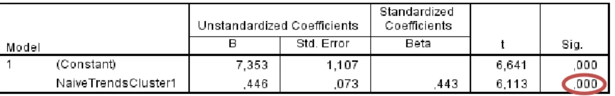
In order to benchmark the results, the naïve approach is used. Three new variables are created with trends based on this approach, one for each cluster. Then a linear regression with the sales of the corresponding cluster is performed. The results for cluster 1 are shown in Table 7. R-square equals 0.196 and the result is significant at a 0.01 level. Cluster 2 shows an R-square value of 0.296 and a significance of p < 0.01. For cluster 3, R-square equals 0.193 with a significance of p < 0.01.
Table 7: Naïve approach for predicting sales numbers of cluster 1 (N = 156)
The results of the linear regression analysis using the naïve approach are compared with the results of linear regression with Google Trends data adjusted for time lag. The predictions for all three clusters have a higher R-square value when using Google Trends data with time lag, the values are reported in Table 8.
Cluster Linear Regression using naïve
approach Linear Regression with Google Trends data adjusted for time lag
Changes
R-square Significance R-square Significance R-square
≤ 32” 0.196 0.000 0.232 0.000 +3.6%
32” < X < 46” 0.296 0.000 0.308 0.000 +1.2%
≥ 46” 0.193 0.000 0.338 0.000 +14.5%
Table 8: Differences between predictions using the naïve approach and Google Trends data
37
5 Discussion and conclusion
5.1 Key findings
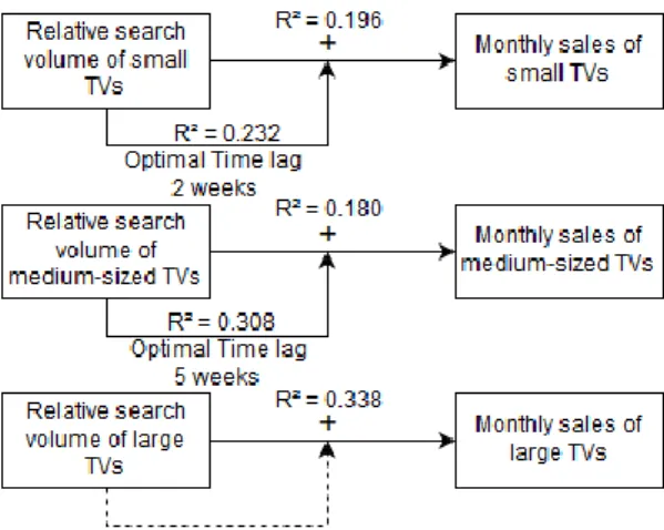
The goal of this research was to develop a reliable prediction method for electronic consumables for a company, using information from search queries on Google Trends. Three hypotheses were tested and the results were benchmarked using the naïve approach. The first hypothesis ‘the number of TV sales increases when the number of searches on Google related to the TV models increases’ is supported by the analysis. For all models approximately 70% (R-square = 0.693) of the variance in the sales variable is explained by the trends. The results for each cluster can be found in Figure 6. The second hypothesis ‘the longer the optimal time lag between tipping points the weaker is the relationship between trends and sales’ could also be supported. However, using monthly data, no time lag could be found, therefore weekly Google Trends and sales data are used. It was found that for the cluster of the smallest TVs, the R-square could be improved to 0.232 from the initial 0.196, by introducing a time lag of two weeks into the relationship. For the cluster of medium-sized TVs, R-square increased from 0.180 to 0.308 after including a time lag of five weeks. For the third cluster with the largest TVs, there was no improvement when introducing a time lag. Overall in two out of three cases, the hypothesis was supported. The third hypothesis ‘the time lag is expected to be longer for TV models with larger screens’ was rejected because the analysis showed that there was no time lag found for TVs with large screens.
38
5.2 Discussion
Google Trends data can conditionally predict the sales of TVs with a time lag. Other data sources, such as Twitter might have delivered different results. With Twitter, daily trends data would be available, but also daily sales data would have been needed. Under these conditions, a more specific estimation of the length of the time lags would have been possible. However, it is questionable whether enough people talk about the purchase of a specific TV on Twitter, and as already mentioned, the sample is not representative of the population (Mislove et al., 2011). Lassen et al. (2014) showed that predicting the purchase of a product like an iPhone is possible with Twitter. However, the search term ‘iphone’ delivers more results (214 mentions within the last month) than the term ‘tv’ (66 mentions) on the analytic site socialmention.com. Even though most of these posts are not related to a purchase, they can show the general popularity of a product at the moment, which can be an indicator for purchases. When using data from Twitter, the methodology also needs to be adapted to sentiment analysis. Using other data sources, e.g. other social media platforms or blogs could be difficult, because either the volume would be too low or most of the content would not be available for research due to privacy restrictions. Data from other search engines might not be as valid as data from Google because Google has a market share of more than 70% followed by Bing with 11.31% (NetApplications.com, 2016). However using search engine data from the retailer’s website could solve the problem of content validity, because customers searching there might be more likely to have a purchase intention.
Overall, it would be possible to perform this research with other data from other sources as well, if the method is adapted accordingly. Using daily sales numbers from more stores could improve the results. Daily sales numbers could not be used with Google Trends, since only weekly trends data is available there but for Twitter Analytics, daily sales numbers could be useful.
39
5.3 Limitations & future research
This research has several limitations, for example the sales numbers from only one retail chain within two geographical close regions were used. Future research could try to use data from more retailers in different geographical locations and thus increase construct validity of the sales data. Furthermore, using weekly or even daily sales numbers could help identifying the time lag more precisely and increase face validity. In order to test the reliability of the method, the research could be repeated with a sample of the data. Also the selection of the TV models could be changed. In this research the 123 best-selling TVs at the retailer were used but it could also be useful to see whether the same results apply to TVs with fewer sales, as long as a sampling error is excluded. Not everyone who searches for a TV on the Internet will purchase the searched TV in-store; neither did everyone who buys a TV in-store search for the model on the Internet. Also, customers might search for the TV on the Internet after the purchase for technical problem solving. This could distort the data, thus it has the problem of content validity. This could be tested in future by removing these cases and repeat the analysis to see whether R-square increases. The keywords could also be adapted to the needs and wants of smaller customer groups. For example some customers who want to play games on the TV focus more on higher refresh rates and the number of HDMI ports, while the screen size might not be the highest priority.
The results of this research is coherent with the expectations of other authors, e.g. Asur and Huberman (2010), Choi and Varian (2012), that sales of products of consumer interest could be predicted using social media or search engine data. Future research can still focus on improving existing methods and predicting other product purchases. Methods to increase the validity of the data and an explanation of the results are also still missing in research.
5.5 Practical implications
40
screens (≤ 32”) the time is two weeks, for medium-sized TVs (between 32” and 46”) five weeks, and for the group with the largest TVs (≥ 46) there was no time lag found. Thus, using Google Trends data, organisations are able to estimate whether the sales in TVs with specific sizes will increase or decrease two or five weeks in advance, depending on the screen size. So, due to the correlation between sales and search engine activity, organisations should analyse and manage search engine data more extensively. In order to generate competitive advantage using this approach, organisations have to adopt and use search engine analytical tools and thus create predictions of future demand changes and order the TVs correspondingly at their suppliers two or five weeks in advance, as long as this time is sufficient to place an order. This way, if the customer finds in-store what he is searching for, customer satisfaction as well as sales might increase. Unfortunately there was no time lag found for the largest TVs, so their demand changes cannot be predicted beforehand using Google Trends. It is advised to repeat this method every few years to identify changes in the time lag because the average size of TVs is increasing. This method can also be used on other consumer products for which the purchase decision might take some time and that customers might want to search on the Internet to gather more information about. Also the AIDA model, the customer journey model, or the consumer buying process should be considered when making these predictions, in order to explain the difference in time between change in search activity and actual in-store purchase.
41
6 Organisation Summary
Um Verkäufe und das Inventar besser planen zu können, kann es hilfreich sein Verkaufsprognosen zu erstellen. Frühere Studien haben gezeigt, dass mithilfe von Daten aus Suchmaschinen effektive Vorhersagen gemacht werden können. Daten von Google Trends wurden zum Beispiel verwendet um Verkaufszahlen von Autos, das Konsumklima, Reiseziele (Choi & Varian, 2012), und Immobilienpreise (Asur & Huberman, 2010) vorauszusagen. Daher ist anzunehmen dass Google Trends auch im Einzelhandel helfen kann die Produktnachfrage zu prognostizieren. Das Ziel dieser Arbeit ist es für das Unternehmen die Verkäufe von Fernsehern vorauszusagen, damit das Inventar effizienter verwaltet werden kann. Fernseher wurden ausgewählt, weil sie recht groß sind und deshalb viel Platz im Lager beanspruchen. Außerdem sind Fernseher eher kostspielig, so dass Käufe wahrscheinlich von den Kunden im Voraus geplant werden. Es wird erwartet, dass sich Kunden online, via Suchanfrage bei Google, über einen Fernseher informieren wollen, bevor sie diesen im Laden kaufen. Eine Inhaltsvalidität kann nicht gewährleistet werden, da sich nicht alle Kunden online informieren, nicht alle Kunden Google benutzen (Marktanteil von > 70%), und nicht alle Kunden im Geschäft kaufen nachdem sie sich online informiert haben. Dennoch sind Daten von Google Trends einfach zu erlangen und bieten einige Vorteile gegenüber traditionellen Umfragen. So kann man unter Anderem mithilfe von Google Trends mehr Daten in einem kürzeren Zeitraum auswerten als bei den meisten Umfragen.
42
Drei Hypothesen wurden aufgestellt:
1. Die Anzahl der TV Verkäufe steigen, wenn die Anzahl der Suchanfragen zum entsprechenden TV Modell steigen.
2. Wenn man die Zeitdifferenz miteinbezieht wird die Verbindung zwischen Google Trends Daten und Verkäufen stärker.
3. Der Zeitdifferenz ist größer bei TV Modellen mit größeren Bildschirmen.
Die Verkaufszahlen für die Analyse wurden von zehn Filialen eines Einzelhändlers für elektronische Güter bereitgestellt. Die Daten von drei Jahren (156 Wochen) wurden analysiert. 123 Fernsehmodelle wurden in die Analyse miteinbezogen und da nicht alle einzeln analysiert werden konnten, wurden die Modelle in drei Cluster eingeteilt. Die Cluster basierten darauf was potentielle Kunden am ehesten als Suchanfrage eingeben würden, wenn sie sich über Fernseher informieren wollen. Es ist unwahrscheinlich, dass viele Kunden die genauen Namen der Modelle, z.B. Sony KDL-55 W 829 B in eine Suchmaschine eingeben. Da für viele Kunden die Marke und die Größe des Fernsehers am wichtigsten sind, wurden die Cluster nach der Größe der Fernseher eingeteilt. Gruppe 1 beinhaltet alle Modelle von 46“ bis 55“, Gruppe 2 32“ bis 45“, und Gruppe 3 22“-32“. Demnach werden Google Trends Daten für die Suchanfragen ‚22“ TV’, ‚23“ TV’, ‚24“ TV’, usw. gesammelt. In diese Suchanfragen werden automatisch Begriffe wie ‚Samsung’, ‚günstig’, oder ähnliches miteinbezogen wenn sie zusammen mit dem Stichwort gesucht wurden.
Die erste Hypothese, dass die Anzahl der TV Verkäufe steigt, wenn die Anzahl der zugehörigen Suchanfragen steigen, wurde bestätigt. Außerdem beträgt die Zeitdifferenz zwischen Suchanfrage und Verkauf bei den kleinsten Geräten zwei Wochen, bei mittelgroßen Geräten fünf Wochen, und bei den größten Geräten wurde keine Differenz gefunden. Nachdem die Zeitdifferenzen in die Analyse miteinbezogen wurden, wurde die Verbindung zwischen Suchanfragen und Verkäufe deutlicher. Die dritte Hypothese konnte nicht bestätigt werden, da die größten Modelle keine Zeitdifferenz aufwiesen.
43
einen Wettbewerbsvorsprung mit dieser Methode zu erreichen, sollten Unternehmen eine Suchmaschinenanalyse einführen und verwenden, um zukünftig Veränderungen der Nachfrage zu prognostizieren und entsprechend rechtzeitig beim Zulieferer bestellen zu können. Wenn die Kunden somit im Geschäft immer das finden was sie suchen, könnten die Kundenzufriedenheit, sowie die Verkäufe steigen.
44
References
Ahmed, S., Jaidka, K., & Cho, J. (2016). The 2014 Indian elections on Twitter: A comparison of campaign strategies of political parties. Telematics and Informatics, 33, 1071-1087.
Asur, S., & Huberman, B. A. (2010). Predicting the Future with Social Media. Paper presented at the WI-IAT '10 Proceedings of the 2010 IEEE/WIC/ACM International Conference on Web Intelligence and Intelligent Agent Technology, Washington, DC.
Babbie, E. (2013). The Practice of Social Research (13 ed.): Wadsworth, Cengage Learning.
Bollen, J., Mao, H., & Zeng, X. (2011). Twitter mood predicts the stock market. Journal of Computational Science(2), 1-8. doi:10.1016/j.jocs.2010.12.007
Burnap, P., Gibson, R., Sloan, L., Southern, R., & Williams, M. (2016). 140 characters to victory?: Using Twitter to predict the UK 2015 General Election. Electoral Studies, 41, 230-233.
Chen, C., Wen, S., Zhang, J., Xiang, Y., Oliver, J., Alelaiwi, A., & Hassan, M. M. (2016). Investigating the deveptive information in Twitter spam. Future Generation Computer Systems. doi:10.1016/j.future.2016.05.036
Choi, H., & Varian, H. (2012). Predicting the Present with Google Trends. The Economic Record, 88(Special Issue), 2-9. doi:10.1111/j.1475-4932.2012.00809.x
Couper, M. P. (2013). Is the Sky Falling? New Technology, Changing Media, and the Future of Surveys. Survey Research Methods, 7(3), 145-156.
Cui, R., Gallino, S., Moreno, A., & Zhang, D. (2015). The Operational Value of Social Media Information. SSRN.
Facebook. (2016). Our Mission. Retrieved May 23, 2016, from http://newsroom.fb.com/company-info/
González-Ibáñez, R., Muresan, S., & Wacholder, N. (2011). Identifying Sarcasm in Twitter: A Closer Look. Paper presented at the HLT '11 Proceedings of the 49th Annual Meeting of the Association for Computational Linguistics: Human Language Technologies: short papers, Portland, OR.
Google. (2016a). How trends data is adjusted - Trends Help. Retrieved May 19, 2016, from
https://support.google.com/trends/answer/4365533?hl=en&ref_topic=436559 9
Google. (2016b). Privacy Policy - Privacy & Terms. Retrieved May 24, 2016, from https://www.google.de/intl/en/policies/privacy/
Google. (2016c). Search tips for Trends. Retrieved May 24, 2016, from https://support.google.com/trends/answer/4359582?hl=en&ref_topic=436553 0
Google. (2016d). Where Trends data comes from. Retrieved May 19, 2016, from https://support.google.com/trends/answer/4355213?hl=en&ref_topic=436559 9
Gregor, S. (2006). The Nature of Theory in Information Systems. MIS Quarterly, 30(3), 611-642.
45
Hill, S., Benton, A., & Bulte, C. V. d. (2013). When does social network-based prediction work? A large scale analysis of brand and TV audience engagement by twitter users. Paper presented at the Thirty Fourth International Conference on Information Systems, Milan, Italy.
Hyndman, R. J., & Athanasopoulos, G. (2014). Forecasting: Principles & Practice. otexts.com.
Jerath, K., Ma, L., & Park, Y.-H. (2014). Consumer Click Behavior at a Search Engine: The Role of Keyword Popularity. American Marketing Association, 51(4), 480-486. Kinski, A. (2016). Google Trends as Complementary Tool for New Car Sales Forecasting: A
Cross-Country Comparison along the Customer Journey. (Master), University of Twente, Enschede, The Netherlands.
Kotler, P. (2000). Marketing Management, Millenium Edition. Saddle River, NJ.
Kusunose, Y., & Mahmood, R. (2016). Imperfect forecasts and decision making in agriculture. Agricultural Systems, 146, 103-110. doi:10.1016/j.agsy.2016.04.006 Lassen, N. B., Madsen, R., & Vatrapu, R. (2014). Predicting iPhone Sales from iPhone
Tweets. Paper presented at the 18th International Enterprise Distributed Object Computing Conference.
Merton, R. K. (1948). The Self-Fulfilling Prophecy. The Antioch Review, 8(2), 193-210. Mislove, A., Lehmann, S., Ahn, Y.-Y., Onnela, J.-P., & Rosenquist, J. N. (2011).
Understanding the Demographics of Twitter Users. Paper presented at the Proceedings of the Fifth International AAAI Conference on Weblogs and Social Media, Barcelona.
Mitchell, J. (2011). Google Searches vs. Sentiment Analysis: Which Is The Real Zeitgeist?
Retrieved March 18, 2016, from
http://readwrite.com/2011/12/22/google_searches_vs_sentiment_analysis_whi ch_is_the/
Moon, M. A., Mentzer, J. T., & Smith, C. D. (2003). Conducting a sales forecasting audit.
International Journal of Forecasting, 19, 5-25.
Moore, J. (2015). Pragmatism, mathematical models, and the scientific ideal of prediction and control. Behavioural Processes, 114, 2-13. doi:http://dx.doi.org/10.1016/j.beproc.2015.01.007
Moshman, D., & Franks, B. A. (1986). Development of the Concept of Inferential Validity.
Educational Psychology Papers and Publicatios, 53, 153.
Nahmias, S. (2009). Forecasting Production and Operations Analysis (Vol. 6). Santa Clara University: McGrawHill.
NetApplications.com. (2016). Search Engine Market Share. Retrieved July 7, 2016, from
https://www.netmarketshare.com/search-engine-market-share.aspx?qprid=4&qpcustomd=0
Önkal, D., & Muradoglu, G. (1996). Effects of task format on probabilistic forecasting of stock prices. International Journal of Forecasting, 12, 9-24.
Pang, B., & Lee, L. (2008). Opinion Mining and Sentiment Analysis. Foundations and Trends in Information Retrieval, 2, 1-135. doi:10.1561/1500000001
Perrin, A., & Duggan, M. (2015). Americans' Internet Access: 2000-2015. Retrieved 01.07.2016, from http://www.pewinternet.org/2015/06/26/americans-internet-access-2000-2015/