Optimal scaling and diffusion limits for the Langevin algorithm in high dimensions

University of Warwick institutional repository: http://go.warwick.ac.uk/wrap

This paper is made available online in accordance with

publisher policies. Please scroll down to view the document

itself. Please refer to the repository record for this item and our

policy information available from the repository home page for

further information.

To see the final version of this paper please visit the publisher’s website

.

Access to the published version may require a subscription.

Author(s): NS Pillai, AM Stuart and AH Thiery

Article Title: Optimal Scaling and Diffusion Limits for the Langevin

Algorithm in High Dimensions

Year of publication: 2011

Link to published article:

http://www2.warwick.ac.uk/fac/sci/statistics/crism/research/2011/paper

11-08

Optimal Scaling and Diffusion Limits for

the Langevin Algorithm in High Dimensions

Natesh S. Pillai, Andrew M. Stuart, Alexandre H. Thi´ery

Department of Statistics, Harvard University MA, USA 02138-2901 e-mail:[email protected]

Mathematics Institute Warwick University

CV4 7AL, UK

e-mail:[email protected]

Department of Statistics Warwick University

CV4 7AL, UK

e-mail:[email protected]

Abstract: The Metropolis-adjusted Langevin (MALA) algorithm is a sampling algorithm which makes local moves by incorporating information about the gradient of the target density. In this paper we study the efficiency of MALA on a natural class of target measures supported on an infinite dimensional Hilbert space. These natural measures have density with respect to a Gaussian random field measure and arise in many applications such as Bayesian nonparametric statistics and the theory of conditioned diffusions. We prove that, started at stationarity, a suitably interpolated and scaled version of the Markov chain corresponding to MALA converges to an infinite dimensional diffusion process. Our results imply that, in stationarity, the MALA algorithm applied to anN−dimensional approximation of the target will takeO(N13) steps to explore the invariant measure. As a by-product of the diffusion limit it also follows that the MALA algorithm is optimized at an average acceptance probability of 0.574. Until now such results were proved only for targets which are products of one dimensional distributions, or for variants of this situation. Our result is the first derivation of scaling limits for the MALA algorithm to target measures which are not of the product form. As a conse-quence the rescaled MALA algorithm converges weakly to an infinite dimensional Hilbert space valued diffusion, and not to a scalar diffusion.The diffusion limit is proved by showing that a drift-martingale decomposition of the Markov chain, suitably scaled, closely resembles an Euler-Maruyama discretiza-tion of the putative limit. An invariance principle is proved for the Martingale and a continuous mapping argument is used to complete the proof.

1. Introduction

Sampling probability distributions in_RN _{forN large is of interest in numerous applications arising in applied}

probability and statistics. The Markov chain-Monte Carlo (MCMC) methodology [RC04] provides a frame-work for many algorithms which effect this sampling. It is hence of interest to quantify the computational cost of MCMC methods as a function of dimensionN. The simplest class of target measures for which such an analysis can be carried out are perhaps target distributions of the form

dπN

dλN(x) = Π N

i=1f(xi). (1.1)

Here λN_{(dx) is the N-dimensional Lebesgue measure and f(x) is a one-dimensional probability density}

function. ThusπN _{has the form of an i.i.d. product.}

Consider aπN_{−invariant Metropolis Hastings Markov chainx}N ₌

xk,N

k≥1which employs local moves,

i.e., the chain moves from current statexk,N _{to a new statex}k+1,N _{via proposing a candidateyaccording to a}

proposal kernelq(xk,N, y) and accepting the proposed value with probabilityα(xk,N, y) = 1∧π_πNN(₍y_x)₎q_q(₍y,x_xk,Nk,N_,y)₎.

Brownian motion)

y=xk,N+√δZN, ZN ∼N(0,IN), (1.2)

and the Langevin proposal (obtained from the time discretization of the Langevin diffusion)

y=xk,N+δlog(πN(xk,N)) +√2δZN, ZN ∼N(0,IN). (1.3)

Here 2δ is the proposal variance, a small parameter representing the discrete time increment. The Markov chain corresponding to the proposal (1.2) is the Random walk Metropolis (RWM) algorithm [MRTT53], and the Markov transition rule constructed from the proposal (1.3) is known as the Metropolis adjusted Langevin algorithm (MALA) [RC04].

A fruitful way to quantify the computational cost of these Markov chains which proceed via local moves is to determine the “optimal” size of incrementδas a function of dimensionN (the precise notion of optimality is discussed below). To this end it is useful to define a continuous interpolant of the Markov chain as follows:

zN(t) = t ∆t−k

xk+1,N+k+ 1− t ∆t

xk,N, for k∆t≤t <(k+ 1)∆t. (1.4)

The proposal variance is 2`∆t, with ∆t=N−γ <sub>setting the scale in terms of dimension and the parameter`</sub>

a “tuning” parameter which is indepedent of the dimensionN. Key questions, then, concern the choice ofγ

and`. These are addressed in the following discussion.

If zN _{converges weakly to a suitable stationary diffusion process then it is natural to deduce that the}

number of Markov chain steps required in stationarity is inversely proportional to the proposal variance, and hence to ∆t,and so grows like Nγ_{. A research program along these lines was initiated by Roberts and}

coworkers in the pair of papers [RGG97,RR98]. These papers concerned the RWM and MALA algorithms respectively. In both cases it was shown that the projection ofzN _{into any single fixed coordinate direction}

xiconverges weakly inC([0, T];R) toz, the scalar diffusion process

dz

dt =h(`)[logf(z)]

0₊p

2h(`)dW

dt . (1.5)

Hereh(`) is a constant determined by the parameter`from the proposal variance. For RWM the scaling of the proposal variance to achieve this limit is determined by the choice γ= 1 ([RGG97]) whilst for MALA

γ=1₃ ([RR98]). These analyses show the number of steps required to sample the target measure grows asN

for RWM, but only asN13 for MALA. The MALA proposal is more sophisticated than the RWM proposal

as the MALA proposal incorporates information about the target density by via the log gradient term (1.3). The optimal scaling results mentioned enable us to quantify the efficiency gained by the MALA compared to that of RWM by employing “informed” local moves using the gradient of the target density. A second important feature of the analysis is that it suggests that the optimal choice of`is that which maximizesh(`). This value of`leads in both cases to a universal optimal average acceptance probability (to three significant figures) of 0.234 for RWM and 0.574 for MALA. These theoretical analyses have had a huge practical impact as the optimal acceptance probabilities send a concrete message to practitioners: one should “tune” the proposal variance of the RWM and MALA algorithms so as to have acceptance probabilities of 0.234 and 0.574 respectively. The criteria of optimality used here is defined on the scale set by choosing the largest proposal variance, as a function of dimension, which leads toO(1) acceptance probability, as the dimension grows. A simple heuristic suggests the existence of such an “optimal scale”. Smaller values of the proposal variance lead to high acceptance rates but the chain only moves locally and therefore may not be efficient. Larger values of the proposal variance lead to global proposal moves, but then the acceptance probability is tiny. The optimal scale for the proposal variance strikes a balance between making large moves and still having a reasonable acceptance probability. Once on this optimal scale, a diffusion limit is obtained and a further optimization, with respect to`, leads the optimal choice of acceptance probability.

Although the optimal acceptance probability and the asymptotic diffusive behavior derived in the original papers of Roberts and coworkers required i.i.d product measures (1.1), extensive simulations (see [RR01,

research [B´ed07, B´ed09,BPS04,BR00,CRR05] confirmed this in slightly more complicated models such as products of one dimensional distributions with different variances and elliptically symmetric distributions, but the diffusion limits obtained were essentially one dimensional. This is because if one considers target distributions which are not of the product form, the different coordinates interact with each other and therefore the limiting diffusion must take values in an infinite dimensional space.

Our perspective on these problems is motivated by applications such Bayesian nonparametric statistics, for example in application to inverse problems [Stu10], and the theory of conditioned diffusions [HSV10]. In both these areas the target measure of interest, π, is on an infinite dimensional real separable Hilbert space Hand, for Gaussian priors (inverse problems) or additive noise (diffusions) is absolutely continuous with respect to a Gaussian measureπ0 on H with mean zero and covariance operator C. This framework for the analysis of MCMC in high dimensions was first studied in the papers [BRSV08,BRS09,BS09]. The Radon-Nikodym derivative defining the target measure is assumed to have the form

dπ

dπ0(x) =MΨexp(−Ψ(x)) (1.6)

for a real-valued π0−measurable functional Ψ : Hs _7→

R, for some subspace Hs contained in H; here

MΨ is a normalizing constant. We are interested in studying MCMC methods applied to finite dimensional approximations of this measure found by projecting onto the firstNeigenfunctions of the covariance operator

C.

It is proved in [DPZ92, HAVW05, HSV07] that the measure π is invariant for H−valued SDEs (or stochastic PDEs – SPDEs) with the form

dz

dt =−h(`) z+C∇Ψ(z)

+p2h(`)dW

dt , z(0) =z

0 _(1.7)

where W is a Brownian motion (see [DPZ92]) in H with covariance operator C. In [MPS09] the RWM algorithm is studied when applied to a sequence of finite dimensional approximations ofπas in (1.6). The continuous time interpolant of the Markov chainZN _{given by (1.4) is shown to converge weakly tozsolving}

(1.7) inC([0, T];Hs_{). Furthermore, as for the i.i.d target measure the scaling of the proposal variance which}

achieves this scaling limit is inversely proportional to N and the speed of the limiting diffusion process is maximized at the same universal acceptance probability of 0.234 that was found in the i.i.d case. Thus, remarkably, the i.i.d. case has been of fundamental importance in understanding MCMC methods applied to complex infinite dimensional probability measures arising in practice.

The purpose of this article is to develop such an analysis for the MALA algorithm. The above mentioned papers primarily study the RWM algorithm. To our knowledge, the only paper to consider the optimal scaling for the Langevin algorithm for non-product targets is [BPS04], in the context of non-linear regression. In [BPS04] the target measure a structure similar to that of the mean field models studied in statistical mechanics so that the target measures behave asymptotically like a product measure when the dimension goes to infinity. Thus the diffusion limit obtained in [BPS04] is finite dimensional.

The main contribution of our work is the proof of a scaling limit of the Metropolis adjusted Langevin algorithm to the SPDE (1.7), when applied to target measures (1.6) with proposal variance inversely pro-portional toN13. Moreover we show that the speedh(`) of the limiting diffusion is maximized for an average

acceptance probability of 0.574, just as in the i.i.d product scenario [RGG97]. Thus in this regard, our work is the first genuine extension of the remarkable results in [RR98] for the Langevin algorithm to target measures which are not of the product form, confirming the results observed from simulation. Recently, in [MPS09], the first two authors developed an approach for deriving diffusion limits for such algorithms. This approach to obtaining invariance principles for Markov chains yields insights into the behavior of MCMC algorithms in high dimensions. In this paper we further develop this method and we believe that the techniques developed here can be built on to derive scaling limits for other popular MCMC algorithms.

In section 2 we set-up the mathematical framework that we adopt througout, and define the version of the MALA algorithm which is the object of our study. Section3 contains statement of the main theorem, and we outline the proof strategy. Section4is devoted to a variety of key estimates, in particular to quantify a Gaussian approximation in the acceptance probability for MALA and, using this, estimates of the mean

drift and diffusion. Then, in section5, we combine these preliminary estimates in order to prove the main theorem. We end, in section6, with some concluding remarks about future directions.

2. MALA Algorithm

In this section we introduce the Karhunen-Lo´eve representation used throughout the paper, and define the precise version of the MALA algorithm that we study in detail. Throughout the paper we use the following notation in order to compare sequences and to denote conditional expectations.

• Two sequences{αn}and {βn} satisfyαn .βn if there exists a constant K >0 satisfying αn≤Kβn

for alln≥0. The notationsαn βn means thatαn.βn andβn.αn.

• Two sequences of real functions{fn}and{gn}defined on the same setDsatisfyfn.gnif there exists

a constantK >0 satisfyingfn(x)≤Kgn(x) for alln≥0 and allx∈D. The notationsfn gnmeans

that fn.gn andgn.fn.

• The notationExf(x, ξ)denotes expectation with respect toξwith the variablexfixed.

2.1. Karhunen-Lo`eve Basis

LetHbe a separable Hilbert space of real valued functions with scalar product denoted byh·,·iand associated normkxk2_{=hx, xi. LetC be a positive, trace class operator onHand {ϕ}

j, λ2j} be the eigenfunctions and

eigenvalues ofC respectively, so that

Cϕj=λ2jϕj, j∈N.

We assume a normalization under which {ϕj} forms a complete orthonormal basis in H, which we refer

to us as the Karhunen-Lo`eve Basis. We assume throughout the sequel that the eigenvalues are arranged in decreasing order.

Any functionx∈ Hcan be represented in the orthonormal eigenbasis ofC via the expansion

x= ∞

X

j=1

xjϕj, xj

def

=hx, ϕji. (2.1)

Throughout this paper we will often identify the function x with its coordinates {xj}∞j=1 ∈ `

2 _{in this}

eigenbasis, moving freely between the two representations. Note, in particular, that C is diagonal with respect to the coordinates in this eigenbasis. By the Karhunen-Lo`eve expansion [DPZ92], a realization x

from the Gaussian measure π0 can be expressed by allowing the xj to be independent random variables

distributed asxj ∼N(0, λ2j).Thus, in the coordinates{xj}∞j=1, the priorπ0in (1.6) has a product structure.

For the particular MALA algorithm studied in this paper we assume that the eigenpairs{λ2

j, ϕj}are known

so that sampling fromπ0is straightforward.

The measureπis absolutely continuous with respect toπ0 and hence any almost sure property underπ0

is also true underπ. For example, it is a consequence of the law of large numbers that, almost surely with respect toπ0,

1

N

N

X

j=1 x2_j

λ2

j

→1 as N → ∞. (2.2)

This, then, also holds almost surely with respect toπ, implying that a typical draw from the target measure

πmust behave like a typical draw fromπ0in the largejcoordinates. It is this structure which creates the link between the original results proven for product measures, and those we prove in this paper. In particular this structure enables us to exploit the product structure of the underlying Gaussian measure, when represented in the Karhunen-Lo`eve coordinate system.

For every x∈ H we have the representation (2.1). Using this expansion, we define Sobolev-like spaces Hr_{, r∈}

R, with the inner-products and norms defined by

hx, yir

def

= ∞

X

j=1

j2rxjyj, kxk2r

def

= ∞

X

j=1

j2rx2_j. (2.3)

Notice thatH0_{=Hand so that the Hinner-product and norm are given byh·,·i=h·,·i}

0 andk · k=k · k0.

FurthermoreHr_{⊂ H ⊂ H}−r_{for anyr >0. The Hilbert-Schmidt normk · k}

C is defined as

kxkC=

X

j

λ−_j2x2j.

Forr∈R, letBr:H 7→ Hdenote the operator which is diagonal in the basis{ϕj}with diagonal entriesj2r,

i.e.,

Brϕj =j2rϕj

so thatB12

r ϕj=jrϕj. The operatorBrlets us alternate between the Hilbert spaceHand the Sobolev spaces

Hr_{via the identities:}

hx, yir=hB

1 2

rx, B

1 2

ryi and kxk2r=kB

1 2

rxk2. (2.4)

Since kBr−1/2ϕkkr = kϕkk = 1, we deduce that {B

−1/2

r ϕk}k≥0 form an orthonormal basis for Hr. For a

positive, self-adjoint operatorD:H 7→ H, we define its trace inHr _by

TrHr(D)def=

∞

X

j=1

h(B−

1 2

r ϕj), D(B

−1 2

r ϕj)ir. (2.5)

Since TrHr(D) does not depend on the orthonormal basis, the operator D is said to be trace class inHr if

TrHr(D)<∞for some, and hence any, orthonormal basis ofHr. Let⊗_Hr denote the outer product operator

inHr _{defined by}

(x⊗Hry)z

def

=hy, zirx ∀x, y, z∈ Hr. (2.6)

For an operatorL:Hr_{7→ H}l_{, we denote the operator norm by}

kLkL(Hr_,Hl₎

def

= sup kxkr=1

kLxkl.

For self-adjointLandr=l= 0 this is, of course, the spectral radius ofL.

Let π0 denote a mean zero Gaussian measure on H with covariance operator C, i.e., π0 def= N(0, C). If

x∼Dπ0, then thexj in (2.1) are independentN(0, λ2j) Gaussians and we may write (Karhunen-Lo´eve)

x= ∞

X

j=1

λjρjϕj, withρj

D

∼N(0,1) i.i.d. (2.7)

Because{Br−1/2ϕk}k≥0 form an orthonormal basis forHr, we may also write (2.7) as

x= ∞

X

j=1

(λjjr)ρj(Br−1/2ϕj), withρj

D

∼N(0,1) i.i.d. (2.8)

Define

Cr=BrC=B1r/2C B

1/2

r . (2.9)

Let Ω denote the probability space in which the sequences{ρj}j∈Nare defined. Then the series in (2.7) may

be shown to converge inL2_(Ω;Hr_{) as long as}

TrHr(C_r) =

∞

X

j=1

λ2_jj2r<∞.

The induced distribution ofπ0 onHr _{is then identical to that of a centered Gaussian measure onH}r _with

covariance operatorCr in the sense that, ifξ

D

∼π0, thenEhξ, uirhξ, vir

=hu, Crvir foru, v∈ Hr. Thus in

what follows, we freely alternate between the Gaussian measures N(0, C) onHand N(0, Cr) onHr.

Our goal is to sample from a measureπ onH, given by (1.6) with π0 as constructed above. Frequently

in applications the function Ψ may not be defined on all ofH, but only on a subspace Hr _{⊂ H, for some}

exponent r > 0. Even though the Gaussian measure π0 is defined on H, depending on the decay of the

eigenvalues of C, there exists an entire range of values ofr such that TrHr(Cr)<∞ so that the measure

π0 has full support onHr_{, i.e.,π0(H}r_{) = 1. From now onwards we fix a distinguished exponent s >0 and}

assume that Ψ : Hs _→

R and that TrHs(C_s) <∞. Then π₀

D

∼ N(0, C) on H and π(Hs_{) = 1. For ease of}

notation we define

ˆ

ϕk =B

−1 2

s ϕk

so that we may viewπ0as a Gaussian measure N(0, Cs) on Hs,h·,·is

, and{ϕˆk}form an orthonormal basis

of Hs_,h·,·i s.

A Brownian motion {W(t)}t≥0 in Hs with covariance operatorCs:Hs→ Hs is a continuous Gaussian

process with stationary increments satisfying EhW(t), xishW(t), yis

= thx, Csyis. For example, taking

{βj(t)} independent standard real Brownian motions, the process

W(t) =X

j

(jsλj)βj(t) ˆϕj (2.10)

is a Brownian motion inHs _{with covariance operatorC}

s; equivalently, this same process{W(t)}t≥0 can be

described as a Brownian motion in Hwith covariance operator equal to C since Equation (2.10) may also be expressed as

W(t) =X

j

λjβj(t)ϕj

.

To approximateπandπ0 by finiteN-dimensional measures πN andπN₀ living in

XN def= span{ϕ1,ˆ ϕ2,ˆ · · ·,ϕˆN},

we introduce the orthogonal projection onXN _{denoted byP}N _:Hs_7→XN _{⊂ H}s_{. The function Ψ}N _:XN _7→

Ris defined by ΨN def= Ψ◦PN. The probability distributionπN supported byXN is defined by

dπN dπN

0

(x) =MΨNexp −ΨN(x)

(2.11)

whereMΨN is a normalization constant andπ₀N is a Gaussian measure supported onXN ⊂ Hs and defined

by the property thatx∼DπN

0 is given by

x=

N

X

j=1

λjξjϕj= (CN)

1 2ξN

where ξj are i.i.d standard Gaussian random variables,ξN = P N

j=1ξjϕj and CN =PN ◦C◦PN. Notice

thatπN _{has Lebesgue density}1_onXN _{equal to}

πN(x) =MΨNexp

−ΨN(x)−1 2kxk

2

CN

(2.12)

where the Hilbert-Schmidt normk · kCN onXN is given by the scalar product

hu, viCN =hu,(CN)−1vi ∀u, v∈XN.

The operatorCN _{is invertible onX}N _{because the eigenvalues ofC are assumed to be strictly positive.}

1_{For ease of notation we do not distinguish between a measure and its density, nor do we distinguish between the}

represen-tation of the measure inXN _{or in coordinates in} RN

2.2. The Algorithm

Define

µ(x) =−x+C∇Ψ(x) (2.13) and

µN(x) =−PNx+CN∇ΨN(x). (2.14) Settingh(`) = 1 in (1.7) we see that the measureπgiven by (1.6) is invariant with the respect to the diffusion process

dz

dt =µ(z) +

√ 2dW

dt , z(0) =z 0

whereW is a Brownian motion (see [DPZ92]) inHwith covariance operatorC. Similarly, the measure πN

given by (2.11) is invariant with respect to the diffusion process

dz dt =µ

N_{(z) +}√₂dW N

dt , z(0) =z

0 _(2.15)

where WN _{is a Brownian motion in Hwith covariance operator C}N_{. The idea of the MALA algorithm is}

to make a proposal based on Euler-Maruyama discretization of a diffusion process which is invariant with respect to the target. To this end we consider, from statex∈XN_{, proposalsy∈X}N _{given by}

y−x=δ µN(x) +√2δ(CN)12_ξN _{where δ=`N}−13 _(2.16)

with ξN ₌ PN

i=1ξiϕi and ξi

D

∼ N(0,1). Thus δ is the time-step in an Euler-Maruyama discretization of (2.15). We introduce a related parameter

∆t:=`−1δ=N−13

which will be the natural time-step for the limiting diffusion process derived from the proposal above, after inclusion of an accept-reject mechanism. The scaling of ∆t, and henceδ,withN will ensure that the average acceptance probability is of order 1 asN grows. The quantity` >0 is a fixed parameter which can be chosen to maximize the speed of the limiting diffusion process: see the discussion in the introduction and after the Main Theorem below.

We will study the Markov chain{xk,N}k≥0resulting from Metropolizing this proposal when it is started

at stationarity: the initial position x0,N is distributed as πN and thus lies in XN. Therefore, the Markov chain evolves inXN; as a consequence, only the firstN components of an expansion in the eigenbasis ofC

are nonzero and the algorithm can be implemented in_RN_{. However the analysis is cleaner when written in}

XN _{⊂ H}s_.

The acceptance probability only depends on the firstN coordinates of xandy and has the form

αN(x, ξN) = 1∧ π

N_(y)TN_{(y, x)}

πN_(x)TN_{(x, y)} = 1∧e

QN(x,ξN)_{. (2.17)}

where the functionTN _{given by}

TN(x, y)∝expn− 1

4δky−x−δµ

N_(x)k2

CN

o

is the density of the Langevin proposals. The local mean acceptance probabilityαN_{(x) is defined by}

αN(x) =ExαN(x, ξN). (2.18)

The Markov chain forxN _={xk,N_{}can also be expressed as}

yk,N =xk,N+δµN(xk,N) +√2δ(CN)12 ξk,N

xk+1,N =γk,Nyk,N+ (1−γk,N)xk,N (2.19)

where ξk,N are i.i.d samples distributed as ξN and γk,N = γN(xk,N, ξk,N) is a Bernoulli random vari-able with success probability αN(xk,N, ξk,N). We may view the Bernoulli random variable as γk,N =

1{Uk_<αN_(xk,N_,ξk,N_)} where Uk

D

∼ Uniform(0,1) is independent from xk,N _{and ξ}k,N_{. The quantity Q}N

de-fined in Equation (2.17) may be expressed as

QN(x, ξN) =−1 2

kyk2

CN − kxk2_CN

−ΨN(y)−ΨN(x) (2.20)

− 1 4δ

n

kx−y−δµN(y)k2

CN − ky−x−δµN(x)k2_CN

o

.

As will be seen in the next section, a key idea behind our proof is that, for largeN, the quantityQN_{(x, ξ}N₎

behaves like a Gaussian random variable independent from the current positionx.

In summary, the Markov chain that we have described in Hs _{is, when projected onto X}N_{, equivalent}

to a standard MALA algorithm on RN for the Lebesgue density (2.12). Recall that the target measure π

in (1.6) is the invariant measure of the SPDE (1.7). Our goal is to obtain an invariance principle for the continuous interpolant (1.4) of the Markov chain{xk,N}started in stationarity,i.e, to show weak convergence inC([0, T];Hs_{) ofz}N_{(t) to the solutionz(t) of the SPDE (1.7), as the dimensionN → ∞.}

3. Diffusion Limit and Proof Strategy

In this section we state the main theorem, set it in context, and explain the proof technique that we adopt.

3.1. Main Theorem

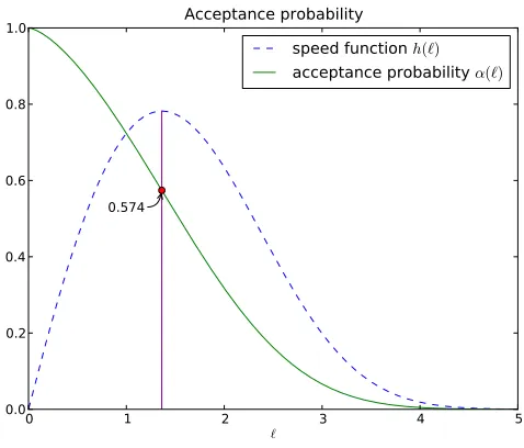
Consider the constantα(`) =E1∧eZ`_{where Z}

`

D ∼N(−`3

4,

`3

2) and define the speed function

h(`) =`α(`). (3.1)

The quantity α(`) represents the limiting expected acceptance probability of the MALA algorithm while

h(`) is the asymptotic speed function of the limiting diffusion. The following is the main result of this article (it is stated in full, with conditions, as Theorem5.2):

Main Theorem: Let the initial condition x0,N _{of the MALA algorithm be such that x}0,N _∼D _πN _{and let}

zN_{(t) be a piecewise linear, continuous interpolant of the MALA algorithm (2.19) as defined in (1.4) with}

∆t=N−13. Then, for anyT >0,zN(t)converges weakly inC([0, T],Hs)to the diffusion process z(t)given

by Equation (1.7)with z(0)∼Dπ.

We now explain the following two important implications of this result:

• since time has to be accelerated by a factor (∆t)−1_=N1

3 in order to observe a diffusion limit, it follows

that in stationarity the work required to explore the invariant measure scales as O(N13);

• the speed at which the invariant measure is explored, again in stationarity, is maximized by tuning the average acceptance probability to 0.574.

The first implication follows from (1.4) since this shows thatO(N13) steps of the MALA Markov chain (2.19)

are required forzN_{(t) to approximatez(t) on a time interval [0, T] long enough forz(t) to have explored its}

invariant measure. The second implication follows from Equation (1.7) forz(t), together with the definition (3.1) ofh(`) itself. The maximum of the speed of the limiting diffusionh(`) occurs at an average acceptance probability of α? _{= 0.574, to three decimal places. Thus, remarkably, the optimal acceptance probability}

identified in [RR98] for product measures, is also optimal for the non-product measures studied in this paper.

0 1 2 3 4 5 `

0.0 0.2 0.4 0.6 0.8 1.0

0.574

Acceptance probability

speed function

acceptance probability

Fig 1. Optimal acceptance probability =0.574

3.2. Proof strategy

To communicate the main ideas, we give a heuristic of the proof before proceeding to give full details in subsequent sections. Let us first examine a simpler situation: consider a scalar Lipshitz functionµ:_R→R

and two scalar constants`, C >0. The usual theory of diffusion approximation for Markov processes [EK86] shows that the sequencexN _{of Markov chains}

xk+1,N−xk,N=µ(xk,N)`N−13 ₊

p

2`N−13 C 1 2_ξk_,

with i.i.d.ξk _∼D _{N(0,1) converges weakly, when interpolated using a time-acceleration factor of N}1

3, to the

scalar diffusiondz(t) =`µ z(t)dt+√2` dW(t) whereW is a Brownian motion with variance Var W(t)=

Ct. Also, if γk is an i.i.d. sequence of Bernoulli random variables with success rate α(`), independent from the Markov chainxN, one can prove that the sequence xN of Markov chains given by

xk+1,N −xk,N =γk nµ(xk,N)`N−13 +

p

2`N−13 C 1 2ξk

o

converges weakly, when interpolated using a time-acceleration factorN13, to the diffusion

dz(t) =h(`)µ z(t)

dt+p2h(`)dW(t) where h(`) =`α(`).

This shows that the Bernoulli random variables γk have slowed down the original Markov chain by a factorα(`).

The proof of Theorem 5.2 is an application of this idea in a slightly more general setting. The following complications arise.

• Instead of working with scalar diffusions, the result holds for a Hilbert space-valued diffusion. The correlation structure between the different coordinates is not present in the preceding simple example and has to be taken into account.

• Instead of working with a single drift functionµ, a sequence of approximationsdN _{converging toµhas}

to be taken into account.

• The Bernoulli random variables γk,N are not i.i.d. and have an autocorrelation structure. On top of that, the Bernoulli random variables γk,N are not independent from the Markov chainxk,N. This is the main difficulty in the proof.

• It should be emphasized that the main theorem uses the fact that the MALA Markov chain is started at stationarity: this in particular implies thatxk,N _∼D _πN _{for any k≥0, which is crucial to the proof}

of the invariance principle as it allows us to control the correlation betweenγk,N _andxk,N_.

The acceptance probability of the proposal (2.16) is equal toαN_{(x, ξ}N_{) = 1∧e}QN(x,ξN)_{and the quantity} αN_{(x) =}

Ex[αN(x, ξN)] given by (2.18) represents the mean acceptance probability when the Markov chain

xN _{stands at x. For our proof it is important to understand how the acceptance probability α}N_{(x, ξ}N₎

depends on the current position x and on the source of randomness ξN_{. Recall the quantity Q}N _defined

in Equation (2.20): the main observation is that QN(x, ξN) can be approximated by a Gaussian random variables

QN(x, ξN) ≈ Z` (3.2)

whereZ`

D ∼N(−`3

4,

`3

2). These approximations are made rigorous in Lemma4.1and Lemma 4.2. Therefore,

the Bernoulli random variableγN(x, ξN) with success probability 1∧eQN(x,ξN) can be approximated by a Bernoulli random variable, independent ofx, with success probability equal to

α(`) =_E

1∧eZ`_{. (3.3)}

Thus, the limiting acceptance probability of the MALA algorithm is as given in Equation (3.3). Recall that ∆t=N−13.With this notation we introduce the drift functiondN :Hs→ Hs given by

dN(x) = h(`)∆t−1Ex1,N −x0,N|x0,N =x (3.4)

and the martingale difference array{Γk,N :k≥0}defined by Γk,N = ΓN(xk,N, ξk,N) with

Γk,N = 2h(`)∆t−

1

2_xk+1,N_−xk,N_{−h(`)∆t d}N_(xk,N_{). (3.5)}

The normalization constanth(`) defined in Equation (3.1) ensures that the drift functiondN _{and the}

mar-tingale difference array{Γk,N_{} are asymptotically independent from the parameter `. The drift-martingale}

decomposition of the Markov chain{xk,N_}

k then reads

xk+1,N−xk,N=h(`)∆tdN(xk,N) +p2h(`)∆tΓk,N. (3.6) Lemma 4.4 and Lemma 4.5 exploit the Gaussian behaviour of QN_{(x, ξ}N_{) described in Equation (3.2) in}

order to give quantitative versions of the following approximations,

dN(x) ≈ µ(x) and Γk,N ≈ N(0, C) (3.7)

whereµ(x) =−x+C∇Ψ(x). From Equation (3.6) it follows that for largeN the evolution of the Markov chain ressembles the Euler discretization of the limiting diffusion (1.7). The next step consists of proving an invariance principle for a rescaled version of the martingale difference array{Γk,N_{}. The continuous process}

WN _∈C([0;T],Hs_{) is defined as}

WN(t) =√∆t

k

X

j=0

Γj,N + t−√k∆t ∆t Γ

k+1,N _{for k∆t≤t <(k+ 1)∆t. (3.8)}

The sequence of processes {WN_{} converges weakly in C([0;T],H}s_{) to a Brownian motion W in H}s _with

covariance operator equal toCs. Indeed, Proposition 4.7proves the stronger result

(x0,N, WN) =⇒(z0, W)

where =⇒ denotes weak convergence in Hs_×C([0;T],Hs_{) and z}0 _∼D _{π is independent of the limiting}

Brownian motion W. Using this invariance principle and the fact that the noise process is additive (the diffusion coefficient of the SPDE (1.7) is constant), the main theorem follows from a continuous mapping argument which we now outline. For anyW ∈C([0, T];Hs_{) we define the Itˆo map}

Θ :Hs×C([0, T];Hs)→C([0, T];Hs)

which maps (z0_{, W) to the unique solution of the integral equation}

z(t) =z0−h(`)

Z t

0

µ(z)du+p2h(`)W(t) ∀t∈[0, T]. (3.9)

Notice thatz= Θ(z0, W) solves the SPDE (1.7). The Itˆo map Θ is continuous, essentially because the noise in (1.7) is additive (does not depend on the statez). The piecewise constant interpolant ¯zN ofxN is defined by

¯

zN(t) =xk for k∆t≤t <(k+ 1)∆t. (3.10)

The continuous piecewise linear interpolantzN _{defined in Equation (1.4) satisfies}

zN(t) =x0,N+h(`)

Z t

0

dN(¯zN(u))du+p2h(`)WN(t) ∀t∈[0, T]. (3.11)

Using the closeness of dN(x) and µ(x), of zN and ¯zN, we will see that there exists a processWcN ⇒W as

N → ∞such that

zN(t) =x0,N −h(`)

Z t

0

µ zN(u)

du+p2h(`)WcN(t),

so that zN _{= Θ(x}0,N_,

c

WN_{). By continuity of the Itˆo map Θ, it follows from the continuous mapping}

theo-rem that zN _{= Θ(x}0,N_,

c

WN_{) =⇒Θ(z}0_{, W) =z as N goes to infinity. This weak convergence result is the}

principal result of this article and is stated precisely in Theorem5.2.

3.3. Assumptions

Here we give assumptions on the decay of the eigenvalues of C – that they decay likej−κ _{for someκ >} 1 2

– and then assumptions on Ψ that are linked to the eigenvalues of C through the need for the change of measure in (2.11) to beπ0−measurable. Let ∇Ψ :Hs_{→ R. Then for eachx∈ H}s _{the derivative∇Ψ(x) is}

an element of the dual (Hs₎∗ _ofHs_{, comprising linear functionals on H}s_{. However, we may identify (H}s₎∗ with H−s _{and view ∇Ψ(x) as an element of H}−s _{for each x∈ H}s_{. With this identification, the following}

identity holds

k∇Ψ(x)kL(Hs_,R)=k∇Ψ(x)k−_s

and the second derivative ∂2_{Ψ(x) can be identified as an element of L(H}s_,H−s_{). To avoid technicalities}

we assume that Ψ(x) is quadratically bounded, with first derivative linearly bounded and second derivative globally bounded. Weaker assumptions could be dealt with by use of stopping time arguments.

Assumptions 3.1. The operator C and functionalΨsatisfy the following:

1. Decay of Eigenvalues λ2

i of C:there is an exponentκ >

1

2 such that

λjj−κ

2. Assumptions on Ψ: There exist constants Mi ∈R, i≤4 ands∈[0, κ−1/2)such that Ψ :Hs→ R

satisfies

M1≤Ψ(x)≤M21 +kxk2s

∀x∈ Hs (3.12)

k∇Ψ(x)k−s≤M3

1 +kxks

∀x∈ Hs (3.13)

k∂2Ψ(x)kL(Hs_,H−s₎≤M4 ∀x∈ Hs. (3.14)

Remark 3.2. The condition κ > 1₂ ensures that C is trace class in H. In fact Cr is trace-class in Hr for

any r < κ−1

2. It follows that the H

r _{norm of x ∼}D _{N(0, C) is π0-almost surely finite for any r < κ−}1 2

becauseE

kxk2

r

= TrHr(C_r)<∞.

Remark 3.3. The functional Ψ(x) = 1₂kxk2

s is defined on H

s _{and its derivative at x ∈ H}s _{is given by}

∇Ψ(x) =P

j≥0j 2s_x

jϕj∈ H−swith k∇Ψ(x)k−s=kxks. The second derivative ∂2Ψ(x)∈ L(Hs,H−s) is the

linear operator that mapsu∈ Hs_to P

j≥0j2shu, ϕjiϕj∈ Hs: its norm satisfies k∂2Ψ(x)kL(Hs_,H−s₎= 1for

any x∈ Hs_.

Since the eigenvalues λ2

j ofC decrease asλj j−κ, the operatorC has a smoothing effect:Cαhgains 2ακ

orders of regularity.

Lemma 3.4. For any vector h∈ Hand exponentβ∈_R,khkC khkκ andkCαhkβ khkβ−2ακ.

Proof. Under Assumption3.1the eigenvalues satisfyλj j−κ. Hence

khk2

C=

X

j≥1

λ−_j2h2_j X

j≥1

j2κh2_i =khk2

κ.

Also,

kCαhk2

β =

X

j≥1

j2βhCαh, ϕji2=

X

j≥1

j2β λ2jαhj

2

X

j≥1

j2βj−4καh2j =khk2β−2ακ,

which concludes the proof of the lemma.

For simplicity we assume throughout this paper that ΨN_{(·) = Ψ(P}N_{·). From this definition it follows}

that ∇ΨN_{(x) =P}N_∇Ψ(PN_{x) and ∂}2_ΨN_{(x) =P}N_∂2_Ψ(PN_x)PN_{. Other approximations could be handled}

similarly. The function ΨN _{may be shown to satisfy the following:}

Assumptions 3.5. The functionsΨN _:Hs_→

Rsatisfy the same conditions imposed onΨgiven by

Equa-tions (3.12),(3.12) and (3.14)with the same constants uniformly in N .

Notice also that the above assumptions on Ψ and ΨN _imply2 _{that for allx, y∈ H}s_,

ΨN(y) = ΨN(x) +h∇ΨN(x), y−xi+ rem(x, y) with rem(x, y)≤M5kx−yk2

s (3.15)

for some constantM5>0. The following result will be used repeatedly in the sequel:

Lemma 3.6. (C∇Ψ :Hs_{→ H}s _{is globally Lipschitz)}

Under Assumptions3.1the functionalCΨis globally Lipschitz on Hs_{: there existsM}

6>0 satisfying

kC∇Ψ(x)−C∇Ψ(y)ks≤M6kx−yks ∀x, y∈ Hs.

Proof. Becauses−2κ <−swe havekC∇Ψ(x)−C∇Ψ(y)ks k∇Ψ(x)−∇Ψ(y)ks−2κ.k∇Ψ(x)−∇Ψ(y)k−s

so that it suffices to prove thatk∇Ψ(y)− ∇Ψ(y)k−s.ky−xks. Assumption3.1states that∂2Ψ is uniformly

bounded inL(Hs_,H−s_{) so that}

k∇Ψ(y)− ∇Ψ(y)k−s=

Z 1 0

∂2Ψ x+t(y−x)

·(y−x)dt

_−s (3.16)

2_{We extendh·,·ifrom an inner-product onHto the dual pairing betweenH}−s_andHs_.

≤

Z 1

0

k∂2Ψ x+t(y−x)

·(y−x)k−sdt

≤M4

Z 1

0

ky−xksdt,

which finishes the proof of Lemma3.6.

Remark 3.7. Lemma3.6 shows in particular that the function µ :Hs _{→ H}s _{defined by (2.13) is globally}

Lipschitz on Hs_{. The same proof shows that C}N_∇ΨN _{: H}s_{→ H}s _{and µ}N _{: H}s_{→ H}s _{given by (2.14) are}

globally Lipschitz and that the Lipschitz constants can be chosen uniformly in N.

The globally Lipschitz property ofµensures that the solution of the Langevin diffusion (1.7) is defined for all time. The global Lipschitzness ofµis also used to show the continuity of the Itˆo map Θ :Hs_{×C([0, T],H}s_)→

C([0, T],Hs_{) which maps (Z}0_{, W)∈ H}s_{×C([0, T],H}s_{) to the unique solution of the integral equation (3.9)}

below.

We now show that the sequence of functionsµN _:Hs_{→ H}s _{defined by}

µN(x) def= −PNx+CN∇ΨN(x)=−PNx+PNCPN∇Ψ(PNx)

converge toµin an appropriate sense.

Lemma 3.8. (µN _{converges π}

0-almost surely to µ)

Let Assumption3.1hold. The sequences of functions µN _satisfies

π0nx∈ Hs_{: lim} N→∞ kµ

N_(x)−µ(x)k s= 0

o

= 1.

Proof. It is enough to verify that forx∈ Hs _{we have}

lim

N→∞kP

N_x−xk

s= 0 (3.17)

lim

N→∞kCP

N_∇Ψ(PN_{x)−C∇Ψ(x)k}

s= 0. (3.18)

• Let us prove Equation (3.17). Forx∈ Hs_{we have} P

j≥1j2sx2j <∞so that

lim

N→∞kP

N_x

−xk2s = lim N→∞

∞

X

j=N+1

j2sx2_j = 0. (3.19)

• Let us prove (3.18). The triangle inequality shows that

kCPN∇Ψ(PNx)−C∇Ψ(x)ks≤ kCPN∇Ψ(PNx)−CPN∇Ψ(x)ks+kCPN∇Ψ(x)−C∇Ψ(x)ks

The same proof as Lemma 3.6reveals that CPN_{∇Ψ :H}s_{→ H}s_{is globally Lipschitz, with a Lipschitz}

constant that can be chosen independent from N. Consequenly, Equation (3.19) shows that

kCPN∇Ψ(PNx)−CPN∇Ψ(x)ks.kPNx−xks→0.

Also, z = ∇Ψ(x) ∈ H−s _{so that k∇Ψ(x)k}2

−s =

P

j≥1j

−2s_z2

j < ∞. The eigenvalues of C satisfy

λ2_j j−2κ withs < κ−1

2. Consequently,

kCPN∇Ψ(x)−C∇Ψ(x)k2

s=

∞

X

j=N+1

j2s(λ2jzj)2.

∞

X

j=N+1

j2s−4κzj2

= ∞

X

j=N+1

j4(s−κ)j−2szj2≤

1

(N+ 1)4(κ−s)k∇Ψ(x)k 2

−s → 0.

The next lemma shows that the size of the jumpy−xis of order√∆t.

Lemma 3.9. Consider y given by (2.16). Under Assumptions3.5, for anyp≥1 we have

Eπ

N

x

ky−xkp s

.(∆t)p2 ·(1 +kxkp

s).

Proof. Under Assumption 3.5 the functionalµN _{is globally Lipschitz on H}s_{, with Lipschitz constant that}

can be chosen independent fromN. Thus

ky−xks.∆t(1 +kxks) +

√

∆tkC12ξNk_s.

We have Eπ

0h

kC12ξNkp

s

i

≤ Eπ

0h

kζkp s

i

< ∞, where ζ ∼D N(0, C). Fernique’s theorem [DPZ92] shows that

Eπ

0h

kζkp s

i

<∞. Consequently,_Eπ0h

kC12ξNkp_s

i

is uniformly bounded as a function ofN, proving the lemma.

The normalizing constantsMΨN are uniformly bounded and we use this fact to obtain uniform bounds

on moments of functionals in Hunder πN. Moreover, we prove that the sequence of probability measures

πN _onHs_{converges weakly inH}s_toπ.

Lemma 3.10. (Finite dimensional approximation πN _ofπ)

Under the Assumptions3.5onΨN the normalization constantsMΨN are uniformly bounded so that for any

measurable functionalf :H 7→R, we have

Eπ

N

|f(x)|

.Eπ0|f(x)|.

Moreover, the sequence of probability measureπN _satisfies

πN =⇒ π

where=⇒ denotes weak convergence inHs_.

Proof. By definition,M_Ψ−N1 =

R

Hexp{−Ψ

N_{(x)}π0(dx)≥}R

Hexp{−M2(1+kxk

2

s)}π0(dx)≥e−2M2P(kxks≤1)

and therefore inf{M_Ψ−N1 : N ∈ N} > 0, which shows that the normalization constants MΨN are

uni-formly bounded. Because ΨN _{is uniformly lower bounded by a constant M1, for any f : H 7→}

R we have

Eπ

N

|f(x)| ≤sup_N

M_ΨN _Eπ0

h

e−ΨN_(x)

|f(x)|i≤e−M1_sup

N

M_ΨN _Eπ0|f(x)|.

Let us now prove that πN _{=⇒π. We need to show that for any bounded continuous function g :H}s_→ R

we have limN→∞ Eπ

N

[g(x)] =Eπ[g(x)] where

Eπ

N

[g(x)] =Eπ

N

0 _[g(x)M

ΨNe−Ψ N_(x)

] =Eπ0_[g(PN_x)M

ΨNe−Ψ(P N_x)

].

Sinceg is bounded, Ψ is lower bounded and since the normalization constants are uniformly bounded, the dominated convergence theorem shows that it suffices to show that g(PNx)MΨNe−Ψ(P

N_x)

converges π0 -almost surely tog(x)MΨe−Ψ(x). For this in turn it suffices to show that Ψ(PN x) convergesπ0-almost surely to Ψ(x) as this also proves almost sure convergence of the normalization constants. By (3.13) we have

|Ψ(PN x)−Ψ(x)|_.(1 +kxks+kPNxks)kPN x−xks.

But limN→∞ kPN x−xks→0 for anyx∈ Hs, by dominated convergence, and the result follows.

Fernique’s theorem [DPZ92] states that for any exponentp≥0 we have Eπ

0

kxkp s

<∞. It thus follows from Lemma3.10that for anyp≥0

sup

N

n

Eπ

N

kxkps

:N ∈N

o

< ∞.

This estimate is repeatedly used in the sequel.

4. Key Estimates

In this section we describe a Gaussian approximation within the acceptance probability for the MALA algorithm and, using this, quantify the mean one-step drift and diffusion.

4.1. Gaussian approximation of QN

Recall the quantityQN _{defined in Equation (2.20). This section proves thatQ}N _{has a Gaussian behaviour}

in the sense that

QN(x, ξN) =ZN(x, ξN) + iN(x, ξN) + eN(x, ξN) (4.1)

where the quantitiesZN andiN are equal to

ZN(x, ξN) =−`

3

4 −

`32

√ 2N

−1 2

N

X

j=1

λ−_j1ξjxj (4.2)

iN(x, ξN) = 1 2(`∆t)

2_kxk2

CN − k(C

N₎1 2ξNk2

CN

(4.3)

withiN and eN small. Thus the principal contribution to QN comes from the random variable ZN(x, ξN). Notice that, for each fixed x ∈ Hs_{, the random variable Z}N_{(x, ξ}N_{) is Gaussian. Furthermore, by virtue}

of (2.2), we have that almost surely with respect tox, the Gaussian distribution approaches that ofZ`

D ∼ N(−`3

4,

`3

2). The next lemma rigorously bounds the error terms e

N_{(x, ξ}N_{) and i}N_{(x, ξ}N_{): we show that i}N

is an error term of order O(N−16) and eN(x, ξ) is an error term of orderO(N− 1

3). In Lemma 4.2we then

quantify the convergence ofZN_{(x, ξ}N_{) toZ} `.

Lemma 4.1. (Gaussian Approximation) Let p≥1 be an integer. Under Assumptions 3.1and 3.5 the error terms iN _andeN _{in the Gaussian approximation (4.1)satisfy}

Eπ

N

|iN(x, ξN)|p

1

p

=O(N−16) and

Eπ

N

|eN(x, ξN)|p

1

p

=O(N−13). (4.4)

Proof. For notational clarity, without loss of generality, we supposep= 2q. The quantity QN _{is defined in}

Equation (2.20) and expanding terms leads to

QN(x, ξN) = I1 + I2 + I3

where the quantitiesI1,I2 andI3 are given by

I1=−1 2 kyk

2

CN− kxk2_CN

− 1

4`∆t kx−y(1−`∆t)k 2

CN− ky−x(1−`∆t)k2_CN

I2=−ΨN(y)−ΨN(x)−1 2

hx−y(1−`∆t), CN∇ΨN(y)iCN − hy−x(1−`∆t), CN∇ΨN(x)i_CN

I3=−`∆t 4

n

kCN∇ΨN(y)k2

CN − kCN∇ΨN(x)k2_CN

o

.

The termI1 arises purely from the Gaussian part of the target measure πN _{and from the Gaussian part of}

the proposal. The two other termsI2 and I3 come from the change of probability involving the functional ΨN. We start by simplifyng the expression forI1, and then return to estimate the termsI2andI3.

I1=−1 2 kyk

2

CN − kxk2_CN

− 1

4`∆t k(x−y) +`∆t y)k 2

CN − k(y−x) +`∆t x)k2_CN

=−1 2 kyk

2

CN − kxk2_CN

− 1

4`∆t 2`∆t[kxk 2

CN− kyk2_CN] + (`∆t)2[kyk2_CN− kxk2_CN]

=−`∆t 4

kyk2

CN − kxk 2

CN

.

The term I1 is O(1) and constitutes the main contribution toQN_{. Before analyzing I1 in more detail, we}

show thatI2 andI3 areO(N−

1 3):

Eπ

N

[I₂2q]

1 2q

=O(N−13) and

Eπ

N

[I₃2q]

1 2q

=O(N−13). (4.5)

• We expandI2and use the bound on the remainder of the Taylor expansion of Ψ described in Equation

(3.15),

I2=−nΨN(y)−[ΨN(x) +h∇ΨN(x), y−xi]o+1

2hy−x,∇Ψ

N_{(y)− ∇Ψ}N_(x)i

+`∆t 2

n

hx,∇ΨN(x)i − hy,∇ΨN(y)io =A1+A2+A3.

Equation (3.15) and Lemma3.9 show that

Eπ

N

[A2₁q]_.EπN[ky−xk4q

s ].(∆t)

2q Eπ

N

[1 +kxk4q

s ].(∆t)

2q _=N−1 3

2q

,

where we have used the fact thatEπ

N

[kxk4q

s ].Eπ0[kxk4sq]<∞. Equation (3.16) proves thatk∇ΨN(y)−

∇ΨN_(x)k

−s.ky−xks. Consequently, Lemma3.9shows that

Eπ

N

[A2₂q]_.Eπ

Nh

ky−xk2q s · k∇Ψ

N_{(y)− ∇Ψ}N_(x)k2q

−s

i

.Eπ

Nh

ky−xk4q s

i

. (∆t)2q Eπ

Nh

1 +kxk4q s

i

.(∆t)2 = N−13

2q

.

Assumption3.5states for anyz∈ Hs_{we havek∇Ψ}N_(z)k

−s.1 +kzks. ThereforeEπ

N

[A2₃q]_.(∆t)2q_.

Putting these estimates together,

Eπ

N

[I₂2q]

1 2q

. Eπ

N

[A2₁q+A₂2q+A2₃q]

1 2q

= O(N−13).

• Lemma 3.6 states CN∇ΨN : Hs _{→ H}s _{is globally Lipschitz, with a Lipschitz constant that can be}

chosen uniformly in N. Therefore,

kCN∇ΨN(z)ks.1 +kzks. (4.6)

SincekCN_∇ΨN_(z)k2

CN =h∇Ψ

N_{(z), C}N_∇ΨN_{(z)i, the bound (3.13) gives}

Eπ

N

I₃2q_.∆t2q E

h

h∇ΨN(x), CN∇ΨN(x)iq_+h∇ΨN_{(y), C}N_∇ΨN_(y)iqi

.∆t2q Eπ

Nh

(1 +kxks)2q+ (1 +kyks)2q

i

.∆t2q _EπNh1 +kxk2sq+kyk

2q s

i

. ∆t2q = N−13

2q

,

which concludes the proof of Equation (4.5).

We now simplify further the expression forI1and demonstrate that it has a Gaussian behaviour. We use the definition of the proposalygiven in Equation (2.16) to expandI1. Forx∈XN we havePNx=x. Therefore, forx∈XN,

I1=−`∆t 4

k(1−`∆t)x−`∆t CN∇ΨN(x) +√2`∆t(CN)12ξNk2

CN− kxk2_CN

=ZN(x, ξN) + iN(x, ξN) + B1 + B2 + B3 + B4.

withZN_{(x, ξ}N_{) andi}N_{(x, ξ}N_{) given by Equation (4.2) and (4.3) and}

B1= `

3

4 1−

kxk2

CN

N

B2=−`

3

4N

−1n_kCN_∇ΨN_(x)k2

CN + 2hx,∇Ψ

N_(x)io

B3= `

5 2

√

2N

−5

6hx+CN∇ΨN(x),(CN)12ξNi_CN B4= `

2

2N

−2

3hx,∇ΨN(x)i.

The quantityZN _{is the leading term. For each fixed value ofx∈ H}s_{the termZ}N_{(x, ξ}N_{) is Gaussian. Below,}

we prove that quantityiN _isO(N−1

6). We now establish that each B_j isO(N− 1 3),

Eπ

N B_j2q

1 2q

= O(N−13) j= 1, . . . ,4. (4.7)

• Lemma 3.10shows that _EπN

[ 1−kxk

2

CN

N

2q

]_.Eπ0_{[ 1−}kxk 2

CN

N

2q

]. Underπ0,

kxk2

CN N

D

∼ ρ

2

1+. . .+ρ2N

N .

where ρ1, . . . , ρN are i.i.d N(0,1) Gaussian random variables. Consequently,Eπ

N

[B₁2q]21q ₌O_(N−12).

• The termkCN_∇ΨN_(x)k2q

CN has already been bounded while provingE

πN_[I2q

3 ].

N−13

2q

. Equation

(3.13) gives the bound k∇ΨN_(x)k

−s . 1 +kxks and shows that Eπ

N

hx,∇ΨN_(x)i2q

is uniformly bounded as a function of N. Consequently,

Eπ

N

B₂2q21q _{= O(N}−1_).

• We have hCN_∇ΨN_(x),(CN₎1

2ξNi_CN =h∇ΨN(x),(CN)

1

2ξNiso that

Eπ

N

[hCN∇ΨN(x),(CN)12ξNi2q

CN] . E

πN

[k∇ΨN(x)k2₋q_s· k(CN)12ξNk2q

s ] . 1.

By Lemma3.10, one can supposex∼Dπ0,

hx,(CN)12_ξNi

CN D ∼ N X j=1 ρjξj.

whereρ1, . . . , ρN are i.i.d N(0,1) Gaussian random variables. Consequently

Eπ

N

hx,(CN)12ξNi2q

CN

1 2q

=

O(N12), which proves that

Eπ

N B2₃q

1 2q

= O(N−56+21_{) =} O_(N−13_).

• The boundk∇ΨN_(x)k

−s.1 +kxksensures that

Eπ

N B₄2q

1 2q

=O(N−23).

Define the quantityeN_{(x, ξ}N_{) =I2+I3+B1+B2+B3+B4so thatQ}N _{can also be expressed as}

QN(x, ξN) = ZN(x, ξN) +iN(x, ξN) +eN(x, ξN).

Equations (4.5) and (4.7) show thateN satisfies

Eπ

N

eN(x, ξN)2q

1 2q

= O(N−13).

We now prove thatiN isO(N−16). By Lemma 3.10,_Eπ

N

[iN(x, ξN)2q]_.Eπ0_[iN_{(x, ξ}N₎2q_{]. Ifx∼}D _{π0 we have}

iN(x, ξN) = `

2

2N −2

3

n

kxk2

CN− k(C

N₎1 2ξNk2

CN o = ` 2 2N −2 3 N X j=1

(ρ2j−ξj2).

whereρ1, . . . , ρN are i.i.d N(0,1) Gaussian random variables. SinceE PNj=1(ρ 2

j−ξ

2

j)

2q

.Nq it follows that

Eπ

N

iN(x, ξN)2q

1 2q

= O(N−23+ 1

2) =O(N− 1

6), (4.8)

which ends the proof of Lemma4.1

The next Lemma quantifies the fact thatZN(x, ξN) is asymptotically independent from the current position

x.

Lemma 4.2. (Asymptotic independence)Let p≥1be a positive integer andf :_R→Rbe a1-Lipschitz

function. Consider error terms eN

?(x, ξ)satisfying

lim

N→∞ E

πN

[eN_?(x, ξN)p] = 0.

Define the functionsf¯N _:

R→Rand the constantf¯∈R by

¯

fN(x) =_Exhf ZN(x, ξN) +eN_? (x, ξN)i

and f¯=_E[f(Z`)].

Then the function fN _{is highly concentrated around its mean in the sense that}

lim

N→∞ E

πNh

|f¯N(x)−f¯|pi= 0.

Proof. Letf be a 1-Lipschitz function. Define the functionF :R×[0;∞)→Rby

F(µ, σ) =_E

f(ρµ,σ)

where ρµ,σ

D

∼N(µ, σ2).

The functionF satisfies

F(µ1, σ1) − F(µ2, σ2)

. |µ2−µ1| + |σ2−σ1|. (4.9)

for any choiceµ1, µ2∈Randσ1, σ2≥0. Indeed,

F(µ1, σ1) − F(µ2, σ2) =

E

f(µ1+σ1ρ0,1) − f(µ2+σ2ρ0,1)

≤ E

h

|µ2−µ1| + |σ2−σ1| · |ρ0,1|

i

.|µ2−µ1| + |σ2−σ1|.

We haveEx[ZN(x, ξN)] =E[Z`] =−`

3

4 while the variances are given by

Var

ZN(x, ξN)

= `

3

2 kxk2

CN

N and Var

Z` = ` 3 2.

Therefore, using Lemma3.10,

Eπ

Nh

f¯N(x)−f¯

pi

=Eπ

Nh Ex

f ZN(x, ξN) +eN? (x, ξN)

−f(Z`)

pi

.Eπ

Nh Ex

f ZN(x, ξN)

−f(Z`)

pi

+ _EπN

|eN_?(x, ξN)|p

=Eπ

Nh F(−

`3

4,Var

ZN(x, ξN)12_)−F(−`

3

4,Var

Z` 1 2₎ pi

+ Eπ

N

|eN_?(x, ξN)|p

.Eπ

Nh Var

ZN(x, ξN)12 _−Var

Z`

1 2

pi

+ Eπ

N

|eN_?(x, ξN)|p

.Eπ0

nkxk2

CN N

o12

−1

p

+ Eπ

N

|eN_?(x, ξN)|p

→ 0

In the last step we have used the fact that if x ∼D π0 then kxk

2

CN

N

D

∼ ρ21+...+ρ 2

N

N where ρ1, . . . , ρN are i.i.d

Gaussian random variables N(0,1) so thatEπ0

n_kxk2

CN

N

o12

−1

p

→0.

Corollary 4.3. Let p≥1 be a positive. The local mean acceptance probability αN(x) defined in Equation (2.18) satisfies

lim

N→∞ E

πN

|αN(x)−α(`)|p

= 0.

Proof. The functionf(z) = 1∧ez _{is 1-Lipschitz andα(`) =}

E[f(Z`)]. Also,

αN(x) =Ex

h

f(QN(x, ξN))i=Exf(ZN(x, ξN) +eN? (x, ξ N₎i

witheN

?(x, ξN) =iN(x, ξN) +eN(x, ξN). Lemma4.1shows that limN→∞ Eπ

N

[eN

?(x, ξ)p] = 0 and therefore

Lemma4.2gives the conclusion.

4.2. Drift approximation

This section proves that the approximate drift functiondN _:Hs_{→ H}s _{defined in Equation (3.4) converges}

to the drift functionµ:Hs_{→ H}s_{of the limiting diffusion (1.7).}

Lemma 4.4. (Drift Approximation):Let Assumptions3.1and3.5hold. The drift functiondN :Hs_{→ H}s

converges to µin the sense that

lim

N→∞E

πNh_kdN_(x)−µ(x)k2

s

i

= 0.

Proof. The approximate drift dN is given by Equation (3.4). The definition of the local mean acceptance probabilityαN(x) given by Equation (2.18) show thatdN can also be expressed as

dN(x) =αN(x)α(`)−1µN(x) + √

2`h(`)−1(∆t)−12_εN_(x)

whereµN_{(x) =−P}N_x+CN_∇ΨN_{(x)and the termε}N_{(x) is defined by}

εN(x) = ExγN(x, ξN)C

1

2_ξN _{= Ex 1}∧_eQ

N_(x,ξN₎

C12_ξN_.

To prove Lemma4.4it suffices to verify that

lim

N→∞E

πNh α

N

(x)α(`)−1µN(x)−µ(x)

2

s

i

= 0 (4.10)

lim

N→∞(∆t) −1

Eπ

Nh

kεN(x)k2

s

i

= 0. (4.11)

• Let us first prove Equation (4.10). The triangle inequality and Cauchy-Schwarz inequality show that

Eπ

Nh α

N_(x)α(`)−1

µN(x)−µ(x)

2

s

i2

.E[|αN(x)−α(`)|4]·Eπ

N

[kµN(x)k4s]

+Eπ

N

[kµN(x)−µ(x)k4

s].