http://wrap.warwick.ac.uk/
Original citation:
Li, Chang-Tsun and Wilson, Roland, 1949- (2007) Unsupervised learning and clustering using a random field approach. Coventry, UK: Department of Computer Science,
University of Warwick. CS-RR-431
Permanent WRAP url:
http://wrap.warwick.ac.uk/61597
Copyright and reuse:
The Warwick Research Archive Portal (WRAP) makes this work by researchers of the University of Warwick available open access under the following conditions. Copyright © and all moral rights to the version of the paper presented here belong to the individual author(s) and/or other copyright owners. To the extent reasonable and practicable the material made available in WRAP has been checked for eligibility before being made available.
Copies of full items can be used for personal research or study, educational, or not-for-profit purposes without prior permission or charge. Provided that the authors, title and full bibliographic details are credited, a hyperlink and/or URL is given for the original metadata page and the content is not changed in any way.
A note on versions:
The version presented in WRAP is the published version or, version of record, and may be cited as it appears here.For more information, please contact the WRAP Team at:
Unsupervised Learning and Clustering
Using a Random Field Approach
Chang-Tsun Li and Roland Wilson
Department of Computer Science University of Warwick Coventry CV4 7AL, UK {ctli, rgw}@dcs.warwick.ac.uk
Abstract
In this work we propose a random field approach to unsupervised machine learning, classifier training and pattern classification. The proposed method treats each sample as a random field and attempts to assign an optimal cluster label to it so as to partition the samples into clusters without a priori knowledge about the number of clusters and the initial centroids. To start with, the algorithm assigns each sample a unique cluster label, making it a singleton cluster. Subsequently, to update the cluster label, the similarity between the sample in question and the samples in a voting pool and their labels are involved. The clusters progressively form without the user specifying their initial centroids, as interaction among the samples continues. Due to its flexibility and adaptability, the proposed algorithm can be easily adjusted for on-line learning and is able to cope with the stability-plasticity dilemma.
1 Introduction
Clustering and machine learning algorithms are in widespread use in the areas of bioinformatics [2], pattern classification [10], data mining [7], image analysis [8], multimedia database indexing [6], etc. The main objective in clustering applications is to group samples / patterns into clusters of similar properties. In the context of supervised classifier training, the labels of the training samples / patterns are known beforehand, making the training or design easier. However, the properties, such as class labels, of the samples may not always be available. In such cases, unsupervised learning algorithms are required to train the classifier based on unlabeled samples.
the learning goes on as the new samples are presented. Off-line learning is in no way capable of coping with such a challenge. This issue makes algorithms with the capability of incremental or on-line learning more desirable. A yet more challenging issue in clustering and learning is that the number of classes / clusters may be unknown throughout the learning process.
Among a wide variety of methods, k-means [7, 10] and fuzzy c-means [1, 2, 9] have been intensively employed in various applications. However, classical k-means and fuzzy c-means clustering methods rely on the user to provide the number of clusters and initial centroid. These requirements impose limitations on the applicability of the methods because the number of clusters may not always be known beforehand and the clustering quality depends heavily on the appropriateness of the initial centroids. Although improved versions of these methods have been reported in some applications, the same inherent limitations still exist. Duda et al. [3] suggested two general ways of circumventing this problem. The first one is to repeat the same k-means or fuzzy c-means clustering method for many different values of k or c, and compare some criterion for each clustering. If a large difference in the criterion values is found between a specific clustering and others, the clustering's value of k or c suggests a good guess of the number of clusters. The second approach starts with treating the first pattern as the only cluster. If the similarity between the next pattern and the centroid of the closest cluster is greater than a pre-specified threshold, the new pattern is merged into that closest cluster and the new centroid of that cluster is re-calculated. Otherwise a new cluster, with the new pattern as the only member, is created. This approach is particularly popular in incremental or on-line learning cases because of its plastic characteristic. Unfortunately, the pre-specified threshold implicitly determines the number of clusters which the algorithm will form. A small threshold results in a great number of clusters, while a large threshold leads to a small number of clusters. The clustering of the second approach is also sensitive to the order of patterns entering the clustering processing. This is the so-called stability-plasticity dilemma [4] and needs addressing.
To work without knowing the number of cluster beforehand, hierarchical clustering has been adopted in many bioinformatic applications [5]. However, its exhaustive way of searching for the closest cluster and requirement of complete sample availability make it unsuitable for on-line learning.
2 Proposed Algorithm
The design of our algorithm is based on the following postulates:
formed voting pool. By random we mean, for each sample, the member samples in its voting pool of are different at different stages.
Coping with the problem of unknown number of clusters by allowing each individual sample to be a singleton cluster and interact with the samples in the voting pool to find its own identity progressively.
The rationale supporting our postulates is that the randomness of the voting pool facilitates global interactions (plasticity) while remaining insensitive to the variable and unreliable centroids.
In our work each n-dimensional sample s is treated as a random variable Xs. The
objective of the learning is to assign an optimal class label xs depending on the
observed data Ys, of s (i.e the sample’s position in the n-dimensional Euclidean
space) and observed data Yr and class labels Xr, for all r in a voting pool Ns
(i.e.∀r∈Ns). This can be formulated as a random field (RF) model
) | ( ) , | , ( ) , , , | ( r r r s r r s s r r s s s r r r r s s s s x X x X P x X x X y Y y Y P N r x X y Y y Y x X P = = = = = = ∝ ∈ = = = = (1)
For the sake of conciseness, we will sometimes use YNs(yNs) and XNs(xNs)to
represent the observed data and class labels of all the samples in Ns, respectively.
2.1. Voting Pool
During each iteration when a sample s is being visited, its voting pool Ns comprising k samples, including the sample (called most-similar or MS) closest to s in the Euclidean space and the sample (called most-different or MD) farthest from s and k – 2 samples selected at random, is formed. Both the most-similar and the most-different samples are the ones encountered in the voting pool since the entire learning process starts. That is, in any iteration, if a voting sample selected at random is more similar to (or more different from) s than the current most-similar
(or most-different) sample, the most-similar (or most-different) sample is replaced by that voting sample.
2.2. Cost Function
The random field model of Eq (1) can also be expressed in a Gibbs form in terms of cost functions ( , | , )
s s s N
N s c
s y y x x
U and ( | )
s
N s p
s x x
U , which are associated with the
functions are dependent on the same set of ‘variables’, by properly integrating the two, we obtain a new model as
) , , , ( ) , , |
( s s Ns s Ns
s s y y x x U N N s
s y y x e
x
P ∝ − (2)
The cost function Us(⋅) is defined in this work as the sum of the pair-wise
potentials between site s and the voting members in Ns:
) , , , ( ) , , , ( =
∑
∈ , s ss s N r N sr s r s r N
s
s x x y y V x x y y
U (3)
where the potential Vs,r is defined, based on the sample distance between samples s
and r as
≠ − = − − = r s r s r s r s r s r s r
s D d x x
x x d D y y x x V if if ) ( ) , , , ( , ,
, (4)
where ds,r = |ys - yr| is the Euclidean distance between samples s and r. D is the
estimated threshold dividing the set of Euclidean distances into intra- and inter-class distances. To estimate D, for each sample, we calculate its distances to m other randomly picked samples and find the minimum and maximum distances (We let m
equal 3 in our experiments). Then two values dw and do are calculated by taking the
average of all the minimum and ⋅ m/2th distances, respectively. Finally, D is defined as
)
(
2 1 o wd
d
D
=
+
(5)2.3. Finding the optimal labels
The optimal label xˆs for a sample s can be stochastically or deterministically
selected according to Eq. (2). In our work we adopt deterministic selection, as such picking a label corresponding to a large value of P(⋅)is equivalent to picking a label corresponding to a small value of Us(⋅). Therefore, the optimal label xˆ s is selected
according to Eq. (6).
)) , , , ( ( min arg ˆ s s s N s N s s x
s U x x y y
Before the first iteration of the labelling process starts, each sample is assigned a label randomly picked from the integer range [1, N], where N is the number of samples (not the number of clusters). Therefore, the algorithm starts with a set of N
singleton clusters without user specifying the number of clusters.
3 On-line Learning
Since the proposed algorithm is not dictated by the pre-specified number of clusters and the current centroids of the clusters, it can be easily adjusted for on-line learning as described below. The new samples are all given unique labels that have not been assigned to any existing samples. That is to say that the new samples are treated as singleton clusters. D in Eq. (5) is updated according to the distances between each new sample and m others as described in Section 2.2. Then the labelling continues based on the new clustering and D.
.
4 Experiments
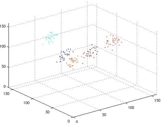
We have applied the proposed algorithm to various sets of 3-dimensional samples consisting of 5 clusters, each having 30 members. The algorithm is tested with the size k of the voting pool set to 4, 6, 10 and 18. In order to get objective statistics during each run of the algorithm, a new sample set is used. For each sample set, the five clusters Ci, i = 1, 2, 3, 4, 5, are randomly created with the 5 centroids fixed at µ1
= (40, 45, 100), µ2 = (85, 60, 100), µ3 =(65, 100, 80), µ4 = (55, 120, 120), µ5 = (120,
50, 120) respectively and the same variance of 64. Figure 1 shows one of the sample set used in our experiments. The clustering performance after repeating the algorithm for 100 times is listed in Table 1. Three cases have been investigated:
1) MS & MD included: This is the case where both most-similar (MS) and most-different (MD) samples are included in the voting pool.
2) MD excluded: This is the case where MS is included while MD is not. An additional random sample is included in place of the MD.
3) MS excluded: This is the case where MS is not included while MD is. An additional random sample is included in place of the MS.
Average iterations and Clustering error rate (%) in Table 1 indicate the average iterations the algorithm have to repeat and percentage of misclassification in one of the 100 runs.
facilitated, as a result, the performance improved even further. One interesting point is that by increasing the number of voting samples from 10 to 18 does not improve the error rate significantly. This suggest that an error rate around 0.4% to 0.8% is the best the algorithm can do given the nature of the sample sets and when such as reasonable error rate is achieved including more voting sample is no longer beneficial because the overall computational load is increased even though the average iteration goes down. For example, apart from other overhead, the computational cost can be measured according to the formula: k ×Average iteration. From Table 1 we can see that the computation costs when k equals10 and 18 are 168 and 193.5, respectively. Such a 0.26 % (= 0.73% – 0.47%) improvement on error rate is not a reasonable trade-off for the 15.18% (= (193.5 – 168) / 168) computational cost in most applications. The optimal size of the voting pool depends on the actual number of clusters and the total number of samples in the data set. Unfortunately, when the proposed algorithm is used in the applications where one or both of the two pieces of information is not unknown, no optimal value of k can be found beforehand.
The second case (MD excluded) is intended to evaluate the performance of the proposed algorithm when the most-different sample is not involved in the voting process. When the size of the voting pool is not big enough (k = 4 and 6 in Table 1) to yield reasonable clustering in terms of clustering error rate, excluding the most-different sample from the voting pool tends to have better performance in terms of average iteration and error rate. That is because the most-different sample is only updated when a more distant sample is found while the additional sample in place of the MD (when the MD is excluded) is picked at random, therefore providing more chances for interaction. However, when the size of the voting pool is big enough (k = 10 and 18 in Table 1) to yield reasonable clustering in terms of clustering error rate, including the most-different sample in the voting pool becomes beneficial in terms of computational cost (average iteration).
The third case (MS excluded) is to demonstrate the importance of the most– similar sample. Note that the most-different sample can only tell the algorithm which particular label not to assign to the sample in question while the most-similar point out which label to assign. Even with the assistance of the MD, without the MS, the algorithm tends to ‘guess’ which label is the correct one. As indicated in Table 1, when k equals 4 and 6 the algorithm never converges. When k is increased to either 10 or 18, successful clustering become possible, however, the computational cost is unacceptably higher than the cases when the MS is included.
average iteration is significantly reduced. This indicates that learning before all the samples are available does occur and it provides the algorithm a point closer to the optimal point in the Euclidean space.
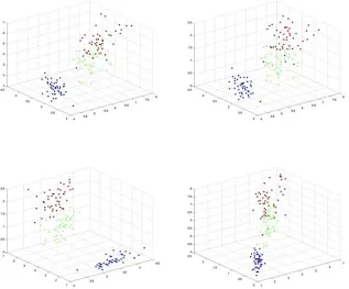
We also tested our algorithm on the well-known Iris dataset. There are three classes of 4 dimensional patterns in the dataset, each having 50 patterns. Since it not possible to visualise 4-D patterns in 2-D media, we have shown the four 3-D plots of the dataset in Figure 2. From Figure 2 we can see that boundaries dividing the three classes do not exist. Consequently, we can expect that clustering error rate will higher when the same algorithm is applied to this dataset. After running the proposed algorithm with the voting pool size k = 10, and the MS and MD included, the average iteration is 23.67 and the average clustering error rate is 6.83%. The best performance in terms of averageclustering error rate is 3%.
5. Conclusions
In this work, we pointed out that learning algorithms may be sensitive to the prior information such as the initial centroids and the number of the clusters and proposed an unsupervised learning algorithm which does not require such prior information and labels of the samples and is capable of on-line learning. The stability-plasticity dilemma and the problem of unknown number of clusters are circumvented through the use of relative similarity between each sample and the member samples in a randomly formed voting pool. The randomness of the voting pool facilitates global interactions (plasticity) while remaining insensitive
References
[1] J. Cui, J. Loewy and E. J. Kendall, “Automated search for arthritic patterns in infrared spectra of synovial fluid using adaptive wavelets and fuzzy c-means analysis, IEEE Transactions on Biomedical Engineering, Vol. 53, No. 5, pp. 800 - 809, May 2006.
[2] D. Dembele and P. Kastner, “Fuzzy c-means method for clustering microarray data,”
Bioinformatics, Vol. 19, No. 8, pp. 973–980, August 2003.
[3] R. Duda, P. Hart and D. Stork, Pattern Classification (second ed.), Wiley, New York, NY, 2000.
[4] S. Grossberg, “Adaptive pattern classification and universal recoding: I. Parallel development and coding if neural feature detectors,” Biological Cybernetics, Vol. 23, pp. 121-134, 1976.
Statistical Association, Vol. 101, No. 473, Applications and Case Studies, pp. 18-29, March 2006.
[6] K. -M. Lee and W. N. Street, “Cluster-driven refinement for content-based digital image retrieval,” IEEE Transactions on Multimedia, Vol. 6, No. 6, pp. 817 – 827, December 2004.
[7] P. Lingras and C. West, “Interval set clustering of web users with rough k-means,”
Journal of Intelligent Information Systems, Vol. 23, No. 1, pp. 5–16, July 2004. [8] K. L. McLoughlin, P. J. Bones and N. Karssemeijer, “Noise equalization for
detection of microcalcification clusters in direct digital mammogram images,” IEEE Transactions on Medical Imaging, Vol. 23, No. 3, pp. 313 – 320, March 2004. [9] N.R. Pal, K. Pal, J.M. Kellerand J.C. Bezdek, “A possibilistic fuzzy c-means
clustering algorithm,” IEEE Transactions on Fuzzy Systems, Vol. 13, No. 4, pp. 517 – 530, August 2005.
[image:9.595.159.442.374.589.2][10] A. Tarsitano, “A computational study of several relocation methods for k-means algorithms,” Pattern Recognition, Vol. 36, No. 12, pp.2955-2966, December 2003.
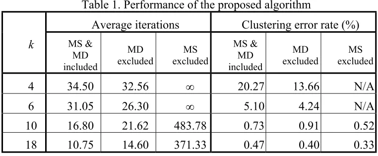
Table 1. Performance of the proposed algorithm
Average iterations Clustering error rate (%)
k MS &
MD included
MD
excluded excluded MS
MS & MD included
MD
excluded excluded MS
4 34.50 32.56 ∞ 20.27 13.66 N/A
6 31.05 26.30 ∞ 5.10 4.24 N/A
10 16.80 21.62 483.78 0.73 0.91 0.52
18 10.75 14.60 371.33 0.47 0.40 0.33
Table 2. Performance of the proposed algorithm in an on-line learning situation.
k Average
iteration Clustering error rate
4 31.77 15.267
6 26.70 4.356
10 12.27 0.711