Public transport on demand : a better match between passenger demand and capacity

(1)

L i t e r a t u r e r e v i e w

M A S T E R ’ S T H E S I S

PUBLIC TRANSPORT ON DEMAND

A better match between passenger demand and capacity

M.H. Matena

(2)

(3)

III

PUBLIC TRANSPORT ON

DEMAND

M.H. (Martijn Hendrik) Matena

Industrial Engineering and Management

Production and Logistic Management

Graduation committee:

Dr. ir. M.R.K. Mes

Dr. ir. J.M.J. Schutten

Dr. ir. H.N. Post

Publication Date:

20 November 2015

University of Twente

Drienerlolaan 5

7522 NB Enschede

The Netherlands

http://www.utwente.edu

Connexxion

Laapersveld 75

1213 VB Hilversum

The Netherlands

(4)

(5)

V

MANAGEMENT SUMMARY

Public transport is becoming more and more important, especially in densely populated cities. The more citizen use public transport, the less congestions and greenhouse gas emissions, which all affect the living environment. But to motivate citizen to use public transport, the public transport service need to be fast, reliable, flexible, and cheap. That is why we formulated the following objective for our research:

Design a solution model that is able to combine and handle real-time DRT requests of customers, with an

acceptable service level against minimal costs.

Connexxion is considering a new solution for the public transport that enables customers to order a ride based on their demand. The current operating bus lines, driving a fixed route, are replaced by a service that creates routes based on the customer demand. The customer has the benefit of no more changes between bus lines, and he or she is able to send a request on a preferred time. We suggest that this model uses predetermined stop locations that are only serviced on-demand. The customers is able to send in a request a short time before the actual start, containing an earliest pickup time. The customer receives a message containing information about the pickup time window, the latest arrival time. A short period before the actual pickup, the exact time of the pickup is communicated. The model is able to make a detour to combine more requests in the same vehicle.

THE TWO MODELS

Inspired by the dial-a-ride problem of Cordeau and Laporte (2003), who formulated a model, that provides a stop-to-stop service with allowed detours to combine rides, we develop a method that is able to handle requests that are only known a short time before the actual pickup. Our model is able to handle on-line requests, this process is explained the figure below.

(6)

VI Connexxion predetermined maximum detour time. For the determination of the maximum detour time, we formulate two models. Model 1 uses a fixed maximum detour time. Independent of the ride length the allowable detour time remains the same. Model 2 uses a detour factor, the allowable detour time is based on the direct ride time times the detour factor. This model results in that all rides have the same relative allowable detour time.

RESULTS

To evaluate the performance of our models, we collected data of the current situation in Helmond. The requests that are used as input for our models, are based on OV-chip card data of September 2015. We are only using requests that stay within Helmond, all requests using bus lines that leave the city are not used. Experiments show that changing parameters have a significant influence on the performances of our models. We see that in the current situation 20 large busses and 4 small vehicles are used. Our results show that only 9 small vehicles with a capacity of eight persons are needed, to serve all requests using one of our models. In the current situation an average distance of 33,452 km, with a corresponding 1,517 hours are needed to serve all requests in a month. Our model 2 serves all the request driving 36,714 km with a corresponding 1,464 hours in a month.

The results show us the effects when serving the customers on demand. Based on de results we believe that the use of on-demand transport is possible, and profitable for Connexxion. Although our model is not extensively tested, we believe if makes a valuable contribution in getting more insight of the possibilities of on-demand transport.

RECOMMEDATIONS AND FURTHER RESEARCH

For the implementation of our on-demand model, we recommend to implement the service in phases. First a combination with the current bus lines, while reducing the frequency of the busses. After a while the bus lines should stop operating and only the on-demand service is available. Since Connexxion already provides the social support transport, the system could combine these requests with the regular request served by on-demand vehicles. To make the service attractive to customers, we recommend to use a fixed fare price.

(7)

M.H. Matena 1

1 INTRODUCTION

“Problems are not stop signs, they are guidelines.” - Robert H. Schuller

This project is commissioned by the department Future Technology (FT) at Connexxion. Connexxion is part of the international shareholder Transdev. The goal of Connexxion is to be the best choice in the field of regional passenger and healthcare transport in the Netherlands. In this chapter, we introduce our research. Section 1.1 provides the context. In Section 1.2, formulates an introduction of our problem, followed by Section 1.3 where we break down the research.

1.1 CONTEXT

Public transport (PT) is getting more and more important in densely populated cities to reduce the number of vehicles on the road. To reduce congestion, citizens need to be stimulated to use PT, instead of using their private car. Congestions causes a lot of stress, loss of time, extra costs, more particulate matter, and accidents. A method to stimulate citizens from not using their private car is a fast, reliable, flexible, and cheap alternative transport mode from one location to another.

The people are expecting a certain level of service from the PT Company, higher service lead most of the times to higher costs, e.g. more buses per hour, increases service, but also increase operation expenses. So a trade-off between operating tasks and the service level must be made. Travelers that use PT want to travel as fast as possible between their pickup location and the destination. The ride of a traveller can be measured in total travel time. The total travel time consists of waiting time, the access and alight time, in-vehicle traveling time and transferring time. Beside the total travel time, the users expect reliable and comfortable rides (Cepeda et al. 2006, Raveau et al. 2011, Schmöcker et al. 2011). The operators are interested in a profitable system, where wages, and the costs of vehicle usage are low.

(10)

[image:10.595.57.541.63.543.2]

2 Connexxion

Figure 1.1: Interactions between the phases of the planning process. (This figure is based on the work of Ibarra-Rojas et al. (2015))

We briefly discuss the phases of the planning process described by Ibarra-Rojas et al. (2015):

 Transit Network Design (TND): the strategic phase, which defines the lines layout with the operational characteristics, e.g. the choice of a vehicle and the space between the stops. In this phase the frequencies must be preliminarily set.

(11)

I n t r o d u c t i o n

M.H. Matena 3

 Transit Network Timetabling (TNT): part of the tactical phase, the times of arrival and departure are determined for all stops along the transit network, to achieve different goals, e.g., meet a given frequency, satisfy specific demand patterns, and maximize the number of well-timed passenger transfers.

 Vehicle Scheduling Problem (VSP): part of the operational phase, determines the assignment of vehicle types to cover all the planned trips with regard to minimizing the operational costs.

 Driver Scheduling Problem (DSP): part of the operational phase, defines the number of duties that cover all the scheduled trips, with regard to the labour regulations, e.g., minimum/maximum work length, while minimizing the cost of driver wages.

 Driver Rostering Problem (DRP): the last part of the operational phase. Given the number of available shifts created in the DSP. The DRP assigns the shifts to the drivers, while satisfying the labour regulations.

Solving the TNP is done in a certain order. Figure 1.1 shows the input data needed to complete a phase. These phases are mostly solved with the use of commercial support packages, such as HASTUS (Rousseau and Blais 1985), HOT II (Daduna and Völker 1995), and TRACS II (Fores et al. 2002). These packages solve the phases (partially) sequentially and can be altered or fine-tuned, by an algorithm or hand, to improve the outcome (Quak 2003).

The creation a complete bus schedule, is a complicated process based on a various number of factors to fulfil the transport demand. A disadvantage of this method is that the schedule is updated only once a year, and the route of the bus is predetermined until a possible new schedule update. Since the routes are set for a certain time period, it could occur that a customer needs to change between buses to get to their destination. The predetermined routes result in a lack of flexibility. If a customer wants flexibility, taxi services can be a better solution. This type of transport can be altered to satisfy the demand of the customer. Taxi services are fast, reliable, and flexible, but are quite expensive and the average number of passengers in the vehicle is low.

The predetermined schedule and lines, as named above, are based on average demand. The demand and supply of transport, can have a misfit in the following ways: the offered capacity is too small, so customers cannot be transported to their destination, or the offered capacity is not used, e.g., empty buses. To reduce this misfit a new approach of PT is needed.

Connexxion is considering a new solution of PT that is able to fulfil the demand. A system that can offer rides on demand makes use of a lot of stop places that are only serviced on demand, and can make agreements about the pickup and delivery times. This new method of PT could solve the misfit to the demand and possibly reduce the number of rides of private cars. The idea is to create a transport solution on demand in which a car or bus drives to the ordered place of the customer. In the literature several names are used for a service like this, namely Demand Responsive Transport (DRT), Demand Responsive Transit, Demand Responsive Service (DRS), Dial-a-ride problem (DARP), or Flexible Transport Services FTS. For the purpose of this research, PT can be categorized as DRT if:

(12)

4 Connexxion  The service uses small vehicles like cars or mini vans.

 The route is created between the requested pickup and drop-off location.

 A request is serviced by a vehicle, if a new request is combined in the same vehicle, the route is changed. If the request cannot be combined, the route is not changed.

 The request can be accepted instantly or pre-booked.

1.2 PROBLEM IDENTIFICATION

On demand transport is commonly only possible with taxi services that are costly for the passengers. A cheaper alternative is to use PT. But travelling to a boarding point to hop on a bus, tram or train is inevitable. Once in PT, the ride is not over the shortest route to the preferred destination, and a change might be needed to transfer to another PT service or line. This generally results in longer travel times compared to direct routes within a city.

The current PT system relies on the Transit Network Planning methodology. This methodology does not take the online demand into account. Hence, a misfit between the offered capacity and the demand may occur. When the bus starts the route it could happen that a lot of customers are travelling from a stop towards a stop in the middle of the route. This can lead to a low utilization of the vehicle, since in the second part of the route no customers are served. Another reason for a lower utilization of buses is that routes cannot be altered to the customer wishes. It could occur that some customers need transfers that can significantly increase the ride time. Customers using PT need, most of the times, extra time to travel towards a stop. The number and location of the stops are pre-set. Compared to a taxi service, where customers are pickup and dropped-off at their preferred address. Customers that want to use the new PT solution still need to travel towards a stop. It is not possible for a customer to enter or leave between stops. If a customer wants to travel, without transit, from and to a specific address, other options can be cycling, using the private car or using a taxi service cab.

(13)

M.H. Matena 5

the new method of PT lies in urban areas when the utilization of bus lines are low, and the travel time to a location is long while the shortest distances between the locations is small.

Connexxion is developing new methods to improve the service for customers, while increasing the utilization of the vehicles. An ultimate goal is to increase the number of travellers using PT. A new more flexible, on demand driven method could be the solution for this challenge.

1.3 RESEARCH PROBLEM

This section describes the research problem. We start with the objective of this research, followed by the scope of the project to finish with the research questions.

1.3.1 OBJECTIVE

The main objective of this research is to develop a solution model that is able to handle the online requests for DRT. The solution model is activated by an online request that is send by the customer. The customer requests the service at least 𝑇𝑟 minutes before the start of the service. The 𝑇𝑟 is to be small, to allow

customers to order the service a short period before the actual start of the service. A request contains the time the customer wants to be picked-up and information about the latest arrival time at the drop-off location. Based on the request data the solution model calculates to which vehicle the customer should be assigned, while not violating the agreements of the customers already in the vehicle.

The solution model are tested with the use of real life, historical data of the Dutch city Helmond and compared to the current situation. In Helmond several scenarios are simulated, e.g., the number of vehicles needed and the capacity of the vehicles. These scenarios are simulated to find improvements or deteriorations and to find out if the new method is cost effective. The simulations are done in Helmond, since a new tender must be written for this area, and a new solution model can be suggested in the tender, if it can operate cost effective. Helmond has several benefits, the area that is covered is relatively small. The area contains, a hospital, a vocational school, and four train stations, this locations probably have a large demand.

The available data of Helmond contains all the rides that are paid with the use of the OV-chip card. This data contributes by the estimation of the demand in Helmond, the travel time within Helmond, and the locations that are often used by travellers. The estimations are used to solve the new solution model. All the simulations done with the new situation, are evaluated on costs effectiveness, to see if a new method for PT can be implemented.

(14)

6 Connexxion

1.3.2 SCOPE

For the development of a solution model, we want to operate within a certain context, of which the boundaries and assumptions are described in this section.

 The pickup and drop-off locations are known. This research is not focussing on finding the optimal locations for the stops points.

 The determination of the shortest path is determined with the use of available software.

 The determination of the travel times is done with the use of a time matrix between stops. The time matrix is created with the use of the shortest path software.

 The vehicles that can be used for our problem, are already purchased. This means that we can only choose between vehicles with a capacity of 3 or 8 persons.

1.3.3 RESEARCH GOAL

In Section 1.3.1, we described the problem of a misfit between the demand and the available capacity. Therefore we define the following research goal:

Design a solution model that is able to combine and handle real-time DRT requests of

customers, with an acceptable service level against minimal costs.

This solution model helps customers to use PT, without changes between lines. Although the solution model uses the current bus stops, these stops are only serviced on demand, and are not serviced in a predetermined order.

1.3.4 RESEARCH QUESTIONS

To achieve the research goal, a number of research questions are formulated. First we start in Chapter 2 by describing the current situation in Helmond. We answer the following questions.

 What is the current route situation in Helmond?  What is the current demand for PT in Helmond?

 What are the costs for driving the routes and what is the utilization?

 How is the current performance measured, and what is the current performance?

Chapter 3 provides a literature study. The literature is used to create a new solution model for the demand responsive transport. We describe the history of the vehicle routing problem followed by the DRT with all restrictions that are needed to handle our case. Then a number of methods for solving routing problems are described.

 What relevant variations of the vehicle routing problem (VRP) are available in the literature?  What solution models are available for DRT?

(15)

M.H. Matena 7

Besides answers on the DRT related questions, Chapter 3 contains a study about factors that influence the service level of the PT, to see what factors are important to improve or maintain. We use the following questions:

 What kind of simulation models can be used for simulating the DRT in Helmond?  How to measure customer satisfaction, and determine fare pricing?

 What can we learn from already implemented DRT systems, what are the advantages and drawbacks?

Chapter 4 describes the solution model, based on the literature discussed in Chapter 3. The following questions are about to be answered:

 How is the solution model formulated?

 What restrictions should be taken into account?

 What solution model is used to solve the model, and have a good performance?

Chapter 5 describes the experiments and the results of the two models.

 What is the performance of the new solution model, in terms of average occupation, driven distance?

(16)

(17)

M.H. Matena 9

2 CURRENT SITUATION

“In business, words are words; explanations are explanations, promises are promises, but only performance is reality”

- Harold S. Genee

This chapter describes the current situation of the Helmond in the Netherlands. The data used for the analysis is the OV chip card data, representing all the check-in/out data. We start this chapter with a Section with a description of Helmond. Section 2.2 describes all stop locations. Section 2.3 describes all the passenger flows in Helmond. Section 2.4 provides the current situation of the bus lines. Section 2.5 describes the utilization of the bus lines. We finalize this Chapter in Section 2.6 with a conclusion about the current situation.

2.1 DESCRIPTION OF HELMOND

Helmond is a historical city in the province of Noord-Brabant in the southern Netherlands. Helmond is one of the five largest cities in the province, with a population of around 90,000, living in an area of 54.75 square kilometre. The population can be divided into several categories as shown in Table 2.1.

Table 2.1: Citizen information of Helmond compared to the province and the country (source: (CBS 2011))

Helmond

Noord-Brabant

Nederland

Citizen

88,291

2,444,158

16,574,989

Age Percentage

-0-20 year

24.9%

23.4%

23.7%

-20-65 year

61.6%

60.9%

61.0%

-65-80+ year

13.3%

15.7%

15.3%

Table 2.1 shows a relative younger population that lives in Helmond, compared to the province and the Netherlands. When changes happen in the PT, younger people are generally able to accept changes faster compared to the elderly (e.g., the implementation of a new PT system).

(18)

[image:18.595.96.501.44.296.2]

10 Connexxion

Figure 2.1: Postal codes in Helmond

2.2 CURRENT BUSSTOPS

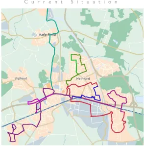
Helmond has 91 bus stops, spread over the municipality. Figure 2.2 shows a map of Helmond where all the stops are shown with a red diamond.

[image:18.595.66.533.398.710.2]

(19)

C u r r e n t S i t u a t i o n

M.H. Matena 11

From Figure 2.1, we see some areas are not covered with bus stops, especially the area above the ‘Bakelse Bossen’ and around ‘Stiphout’. To increase the service level in these areas, transport on demand can be the solution.

2.3 CURRENT PASSENGER FLOWS

To get more insight into the current situation of the demand for public transport in Helmond, we analyse the OV-chip card data. The data is filtered on all the check-ins in Helmond, this also includes intercity bus lines. First we analyse the number of passengers per day, then the demand over the day, to finalize with the number of customers that use the bus lines.

2.3.1 NUMBER OF PASSENGERS PER DAY

[image:19.595.66.540.301.414.2]

To give more insight into the travel behaviour of the citizens of Helmond, we first analyse the number of travellers per day of the week, as shown in Figure 2.3.

Figure 2.3: Number of passengers per day

The figure above clearly shows differences between the working days (Monday – Friday), Saturdays and Sundays. The demand during the workings days is significantly higher than during the weekend. In the first week of September, the demand is lower compared to follow up weeks, in the follow up weeks the demand remains relatively constant. A reason could be that the schools had a start up in the first week. In the weekend, a difference in demand on Saturday and Sunday is at least 41%, were the demand is the lowest at Sundays. In Section 2.3.2, we categorize the days as follows: the working days, Saturdays, and Sundays. We take a closer look at the differences in demand for these three categories.

2.3.2 NUMBER OF PASSENGER CHECK-INS PER HOUR

(20)

[image:20.595.62.540.69.220.2]

12 Connexxion

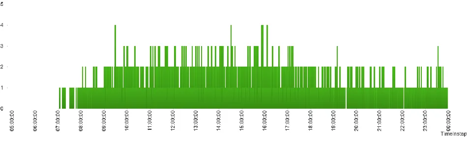
Figure 2.4: Number of passengers traveling per time unit

[image:20.595.59.540.369.552.2]

When we take a closer look at the picture, we clearly see that the customers are traveling in the morning between 6:00 and 9:00, a peak around 14:45, and an increase during from 15:00 to 18:00. After the morning rush the demand for bus transport is slowly increasing until 17:30, after 17:30 a clear drop in demand is noticed. The large peak around 14:45 is caused by students that finished their day at school. Figure 2.4 represents all the demand of September 2015 in Helmond. We analyse the data even further by separating the demand into the following categories: working days (Figure 2.5), Saturdays (Figure 2.6), and Sundays (Figure 2.7).

Figure 2.5: Number of passengers traveling on Monday-Friday per time unit

(21)

[image:21.595.61.539.72.216.2]

M.H. Matena 13

Figure 2.6: Number of passengers traveling on Saturday per time unit

Figure 2.6 (note that the scale is changed) is completely different and do shows a small increase in demand between 9:00 and 19:00. A small decrease of demand is shown before 9:00 and after 19:00. This figure is based on 9,517 check-ins in September 2015. So 4.3% of the rides are made on a Saturday.

Figure 2.7: Number of passengers traveling on Sunday per time unit

Figure 2.7 shows an even further decrease in rides. No clear pattern can be noticed. The demand remains constant during the day. The figure is based on 4,761 check-ins, which equals 2.2% of the total rides done in September 2015.

2.4 THE CURRENT BUS LINES

In this section we describe the current use of buses in Helmond. We start by describing the current bus lines with their frequencies, followed by the operating hours of the bus lines, and finally we describe the type of buses used.

2.4.1 BUS LINES

(22)

14 Connexxion

[image:22.595.150.444.44.342.2]

Figure 2.8: Road map of Helmond showing the current bus lines

Table 2.2: Fares a day in the municipality of Helmond

Bus lines Route colour

(Figure 2.8) Mon/Fri Sat Sun

Line 25 Beek en Donk - Helmond busstation 13 11 4

Line 25 Helmond busstation - Beek en Donk 13 11 4

Line 50 Helmond busstation - Station 't Hout 15 0 0

Line 50 Station 't Hout - Helmond busstation 15 0 0

Line 51 Eeuwsels - Helmond busstation 26 19 0

Line 51 Helmond busstation - Eeuwsels 26 20 0

Line 52 Brouwhuis-Rijpelberg - Helmond busstation 13 9 0

Line 52 Helmond busstation - Brouwhuis-Rijpelberg 11 9 0

Line 53 Straakven - Helmond busstation 12 8 0

Line 53 Helmond busstation - Straakven 11 9 0

Line 54 Brouwhuis - Helmond busstation 14 10 0

Line 54 Helmond busstation - Brouwhuis 11 9 0

Line 54 Straakven - Helmond busstation 10 9 0

Line 54 Helmond busstation - Straakven 12 9 0

Line 552 Helmond busstation - Station Brandevoort 12 9 0

Line 552 Station Brandevoort - Helmond busstation 11 9 0

(23)

M.H. Matena 15

2.4.2 TIMETABLE HOURS

The operating time of a bus line is expressed in timetable hours. Table 2.3 shows the timetable hours of the bus lines and the total distance travelled during the timetable hours.

Table 2.3: Timetable hours per bus line

Line number

Timetable hours

Mon/Fri Sat Sun

Number of days in 2015

Mon/Fri Sat Sun

Total timetable hours a year

Total distance driven a year (KM)

25 9:37

8:09 4:32

255

52

58 3138:59

84,841

50 7:00

0:00 0:00

255

52

58 1785:00

37,426

51 11:58

8:56 0:00

255

52

58 3516:02

66,289

52 6:22

4:47 0:00

255

52

58 1872:14

46,175

53 4:13

3:07 0:00

255

52

58 1237:19

24,563

54 12:10

9:35 0:00

255

52

58 3600:50

73,845

552 10:20

8:06 0:00

255

52

58 3056:12

68,289

Total:

61:40 42:40 4:32

18206:36

401,428

The number of Sundays here is higher than 52 because national holidays also count as Sunday. As mentioned above bus line 51 is the most important line, but in the table above this line has not the most operating hours, this is due the length of the route.

2.4.3 TYPE OF BUSES

The bus lines are served by two type of buses, as shown in Table 2.4.

Table 2.4: Type of buses

Category Bus Capacity Used for Bus Lines Total Number of buses

12 meter bus

45 seats

25, 51, 52, 53, and 54

20 small bus

8 seats

50 and 552

4

It is clear that in the current situation, almost all buses are in the category 12 meter. This bus type is responsible for 13,365 timetable hours, while the small buses are responsible for 4,841 timetable hours. This means that the average time for a 12 meter bus is 668 timetable hours, and 1,210 for a small bus. The small buses are used 44.7% more compared to a 12 meter bus.

The two categories of buses are having different costs. Since some figures are confidential, we use relative costs. We index the costs of the small bus by one. The costs of the 12 meter bus is expressed in the costs of a small bus. These costs are shown in Table 2.5.

Table 2.5: Costs comparison between categories

Category Bus Wages Purchase Costs Depreciation a year Cost per KM Other

12 meter bus

1.58

2.6

3

2 2,5

(24)

16 Connexxion Table 2.5 shows several factors, the first is the wages. Due to the differences in the labour regulations, the driver of a 12 meter bus receives a higher salary. Second and third columns are the purchase costs, and the depreciation costs per year. A larger bus has higher purchase costs and has a depreciation that is three times as high compared to a small vehicle. The cost per kilometre represents the maintenance and fuel. The last column shows all the other costs, e.g., washing, parking, insurance, etc. Comparing the two buses, 2.27 small vehicles have the same costs as one 12 meter bus, if the current bus lines with the same frequency and distance are driven by the smaller vehicles. We conclude that, when more than 16 customers need transport, the 12 meter bus is the preferred solution, else it is cheaper to service the demand with two small vehicles.

2.5 UTILIZATION OF BUSES

We know which bus lines are operating in Helmond, this means that we can filter the OV-chip card data even further to only the trips that are done with bus lines in Helmond. All the intercity lines are left out, since the focus lies on travellers that travel within Helmond. Bus lines 50 and 552 are excluded because the small vehicles used for these lines do not have OV-chip card equipment on board, meaning that there is no available trip data. Figure 2.9 shows the number of passengers traveling by bus in Helmond in the month September 2015.

Figure 2.9: Passengers per bus line

(25)

M.H. Matena 17

Table 2.6: Overview parameters per bus line

Bus line

Total KM Sept.

Number of passengers Passengers per KM Revenue per Line Revenue per KM Season Tickets Season Tickets/ Passengers

KM / stops

25 9,430

755

0.080 660.06 0.069989

248 32.8% 39.6 / 28

50 1,398

-

9.6 / 8

51 48,481

10,470

0.216 3761.68 0.077591

6,599

63.0%

8,7 / 24

52 17,215

1,996

0.116 1438.31 0.083549

825 41.3% 13.0 / 14

53 1,146

2,503

2.185 1321.06 1.153009

1,232

49.2%

8.0 / 22

54 20,585

3,314

0.161 2118.11 0.102895

1,464

44.2% 20.8 / 36

552

856 -

-

18.8 / 40

From Table 2.6 we see that, although bus line 51 is the most important bus line, the revenue per kilometre is not that high. However, the revenue is only based on customers that are not using a season ticket. The revenue generated by season tickets is not assignable to bus lines, because a season ticket gives a traveller the right to travel a certain number of zones. Bus line 51 has the highest percentage of travellers using a season ticket, resulting in a lower revenue per kilometre. When we take a look at the passengers per kilometre, we see that line 53 is the most effective, transporting 2,185 passengers per kilometre, and generating the most revenue per kilometre (excluding the seasonal tickets). Line 53 is effective, even with a relatively small number of travellers, because the complete bus route is only 8 km and contains 22 stops. Bus line 52 performs the worst on the performance indicator, revenue per kilometre.

The following subsections analyse the bus occupation per bus line even further by analysing the top 5 check-in and check-out stops. Since no OV-chip card data is provided from bus lines 50 and 552 no further analyses is done on these lines. Information about the utilization of the buses is described on the basis of average number of passengers in the bus (utilization) per time unit. Section 2.5.1 provides a complete analysis of bus line 25, the follow up section does not show all the graphs, only the noteworthy remarks are done. The graphs are shown in the Appendix B.

[image:25.595.57.530.555.691.2]

2.5.1 BUS LINE 25

Figure 2.10: Top 5 of Check-ins and Check-out locations in bus line 25

(26)

18 Connexxion Station. Most travellers are checking in at Helmond Ziekenhuis, but only a small number are checking out at Helmond Ziekenhuis. A reason could be that a lot of patients use this bus line, and when they need treatment they travel with private transport, and when they are cured they use the bus.

[image:26.595.116.479.145.373.2]

The utilization of bus line 25 is shown in Figure 2.11.

Figure 2.11: Utilization of bus line 25

Figure 2.11 shows that there is a small difference in utilization during the working days and Saturday. There is only a large peak shown around 17:00, the reason for this peak is the closing time of the stores, at this moment the shopping public uses the bus to go home. The utilization for all days is low. A small vehicle has enough capacity to serve all the customers. Since we take the average of the utilization of multiple days, it could happen that the capacity is violated, at certain moments (e.g., when a group of 30 persons are traveling only once a month at 13:00, while all the other days of the month no travellers are using the bus at 13:00. The average utilization at 13:00 is one, but the group cannot fit in the small bus).

2.5.2 BUS LINE 51

Bus line 51 has Helmond Station as most important location, handling a total 4,070 ins and 5,179 check-outs. This difference in travellers could be caused by the several train stations in Helmond, travels that had treatment at the hospital, or the use of intercity buses. Another important location is Helmond Noordende, with 1,460 check-ins and 1,266 check-outs. This stop lies in the city Centre of Helmond, where all stores are located. The shopping public explains the relatively high number of passengers using this stop.

Bus line 51 shows that the utilization during the working days is quite high. The utilization of bus line 51 shows similarities with Figure 2.4, namely the morning rush, an increase in demand around 14:45, and the evening rush. This bus line contains a stop nearby the school that explains the increase in demand at 14:45. We conclude that a 12 meter bus is the right equipment to service all requests during the working days. On

0 0,5 1 1,5 2 2,5 3 3,5 07 :0 0 08 :0 0 09 :0 0 10 :0 0 11 :0 0 12 :0 0 13 :0 0 14 :0 0 15 :0 0 16 :0 0 17 :0 0 18 :0 0 19 :0 0 20 :0 0 21 :0 0 22 :0 0 23 :0 0

Utilization Bus Line 25

(27)

M.H. Matena 19

Saturday no clear pattern can be recognized, but the occupation of the bus is low, and most of the time a smaller bus can be used, but that could lead to rejecting passengers, which is not allowed.

2.5.3 BUS LINE 52

Bus line 52 shows again Helmond Station is the most important location, handling 799 check-ins and 758 of the 1,996 trips.. Another location noteworthy mentioning is Helmond, Deltaweg, since a significant number travellers are traveling towards and from this location. A reason could be that this bus stop is near the train station Helmond Brouwhuis.

Bus line 52 has clear peaks in the utilization, each peak equals a route that is driven by the bus. We see during working days, that the morning the frequency is higher. When comparing the working days with the Saturdays, the utilization remains almost the same. On the Saturdays around 13:00 an even higher utilization is measured. The peak in utilization can be explained by a large group of passengers traveling together around 13:00 using bus line 52. From the utilization data we conclude that the 12 meter bus is the right equipment for this bus line, because the utilization of this bus line is close to the maximum capacity of the small bus.

2.5.4 BUS LINE 53

Bus line 53 has Helmond Station as the most important stop. It handles 396 of the 2,503 check-ins and 412 of the 2,503 check-outs.

Bus line 53 shows an increase in demand on working days in the morning and evening. On the Saturdays, the demand starts high and is slowly decreasing during the day, a reason could be that travellers are leaving Helmond for the weekend in the morning. In this case a 12 meter bus could be the wrong equipment, since the maximum utilization lies around 5, while most of the times it is around 3. Although these numbers are utilization is an average of multiple days, a small bus might do the job.

2.5.5 BUS LINE 54

Bus line 54 shows again that Helmond Station is the most used bus stop, handling 1,496 check-ins, and 1,263 check-outs of 3,314 trips

Bus line 54 shows a unique pattern compared to the other bus lines. We cannot state why this increase in utilization occurs, a reason could be that travellers are traveling back to another train station and make use of bus line 54 to go back home. We see that the utilization is most of the time above 6 travellers. This holds for the working days as well as the Saturdays, only on Saturday mornings a small bus could be used, but the 12 meter bus is the right equipment to meet the demand for the rest of the day.

2.5.6 CONCLUSION

(28)

20 Connexxion bus line is not the most efficient per kilometre. Bus line 53 is the most efficient, but it handles less passengers. We already explained that bus line 51 handles the most season tickets, which is the reason why this bus line has a lower efficiency per kilometre.

2.6 CONCLUSION

From the analysis we see that 19,038 passengers (during a month) are traveling within Helmond. When we analyse the check-in data we clearly see that most transactions are done in the morning rush during the working days, after that period the demand remains steady, with a relatively small increase during the evening period. After the evening, demand declines further until the bus services stop operating. The demand during weekends is a lot smaller and steadier. No rush can be determined only a minor difference between the day shift and the night shift, where the night shows a reduced demand compared to the day.

We state that for some bus lines it is more effective to use smaller buses to service the requests. After 19:00 it is always better to use the small buses. Bus line 51 shows clear rush hours in the utilization of the bus. All the other bus lines do not suffer a significant increase in demand during the morning and/or evening rush, with exception of bus line 54 that only has an evening rush.

The performance of the bus lines varies per bus line, where bus line 53 is the most cost effective, which has 1.15 euro revenue per KM, and having 2,185 passengers per kilometre on board. The frequency of this line is twice per hour, with a total of 23 bus rides during weekdays and 17 bus rides on Saturday. The performance of bus line 51 is not as good as bus line 53, but it handles the most passengers, and it has the highest frequency of 52 busses during the weekdays and 39 busses on Saturdays, a reason for the poor performance is that travellers are only traveling a small part of the complete route.

(29)

M.H. Matena 21

3 LITERATURE REVIEW

“In theory, there is no difference between theory and practice. But in practice, there is.”

- Yogi Berra

In this section of the research, a literature study is performed. We start in Section 3.1 by searching for various problems that are selected to our problem. In the literature our problem is known as the vehicle routing problem (VRP). The vehicle routing problem in general and several variants of the vehicle routing problem are described. Section 3.2 describes several performance indicators and the influence of the performance indicators on the overall customer satisfaction. In Section 3.3 some extensions on the VRP are shown, and the last section of this chapter describes several issues for implementing a demand responsive transport system.

3.1 VEHICLE ROUTING PROBLEMS

More than half a century ago, the VRP was introduced as the truck dispatching problem (Dantzig and Ramser 1959). The VRP is a generic name given to a class of problems involving optimizing vehicle routes. The goal of the VRP is to serve a number of customers with the least amount of vehicles given a set of restrictions, while minimizing the total route costs. Many companies face this problem on a daily basis, think for instance about the supply of stores, or the mail delivery.

The VRP is a combinatorial optimization problem. A combinatorial optimization problem deals with problems of maximizing or minimizing a function with a finite set of solutions. The function of variables subject to inequality and equality constraints and integrally restrictions on some or all of the variables (Wolsey and Nemhauser 2014).

A common formulation for the classical VRP is as follows (Dantzig and Ramser 1959): Let 𝐺 = (𝒱, 𝒜)

be a directed graph where 𝒱 = {0, … , 𝑛} is the vertex set and 𝒜 = {(𝑖, 𝑗): 𝑖, 𝑗 ∈ 𝒱, 𝑖 ≠ 𝑗} is the arc set.

Vertex 0 represents the depot whereas the remaining vertices correspond to customers. A fleet of 𝑚 identical

vehicles with capacity 𝑄 is based at the depot. The fleet size is either given a priori or is a decision variable.

Each customer 𝑖 has a nonnegative demand 𝑞𝑖. A cost matrix 𝑐𝑖𝑗 is defined on 𝒜. The problem consists of

designing 𝑚 vehicle routes such that each route starts and ends at the depot, each customer is visited exactly once by a single vehicle, and the total demand of each route does not exceed 𝑄 (Christofides 1976). A VRP is a generalization of the Traveling Salesman Problem (TSP). The key difference is that in the TSP only one ‘vehicle’ (the salesman) visits a given set of cities with no capacity constraints, while in the VRP a given fleet of 𝑚

vehicles with a capacity 𝑄 that cannot be violated, must visit a given set of customers. In both problems the goal is to find the shortest route, or to minimize the total costs, or to minimize the number of vehicles.

(30)

22 Connexxion Section 3.1.1, in Section 3.1.2 we discuss different solution methods for VRPs, the insertion of customers to known routes are addressed in Section 3.1.3. We end with a conclusion in Section 3.1.4.

3.1.1 VARIANTS OF THE VRP

In case of the classical VRP, some restrictions are not taken into account, this can lead to a mismatch with practice. So over the years new cases of the VRP are proposed. The next sections describe some variations of the classical VRP model.

Vehicle routing problem with time windows

A vehicle routing and scheduling problem with time windows (VRSPTW) or the vehicle routing problem with time windows (VRPTW), deals with allowable delivery times or time windows. The VRSPTW takes the allocations of customers in a present time window into account. In the VRPTW the customers are already allocated to a time window. These variations state that location 𝑖 should be visited within a time

interval [𝐸𝑖, 𝐿𝑖]. A vehicle can arrive at location 𝑖 before time 𝐸𝑖, this means that when vehicle (bus) 𝑏 arrives

too early, it should wait until the time is greater than 𝐸𝑖. If the vehicle arrives too late, i.e., the arrival time is

greater than 𝐿𝑖, the solution is infeasible. The VRPTW can be solved with two objective functions: 1st minimize

the fleet size 𝑚 and the total costs, and 2nd_{minimize the total travel distance or duration of the routes} (Solomon 1987, Bräysy and Gendreau 2005).

Multi-depot vehicle routing problem

The multi-depot vehicle routing problem (MDVRP) is a variation in which there are multiple depot locations. So vehicles can start from different depot locations. The MDVRP has a fleet of vehicles stationed at 𝑧 depots to deliver specified quantities of a single type of product to 𝑛 locations in such a manner that the total distance traveled by the vehicles is minimized (Gillett and Johnson 1976). Since the standard formulation of the MDVRP assumes an unlimited number of vehicles at a depot, a variant on the MDVRP is developed that is called the multi depot vehicle routing problem with fixed distribution of vehicles (MDVRPFD). This variant assigns a fixed number of vehicles to each depot in order to make the algorithm more realistic (Lim and Wang 2005). Another formulation of the MDVRP is with time windows (TW) formulated as a multi-depot heterogeneous fleet vehicle routing problem with TW by Dondo and Cerdá (2007).

Vehicle routing problem with pickup and delivery

A vehicle routing problem with pickup and delivery (VRPPD) is an extension on the classic VRP problem. In the classic VRP, the delivery or the pickup is considered. While the VRPPD handles pickup as well as delivery (e.g., delivering new goods and pickup the return goods). The goal of the VRPPD is to minimize the total distance travelled subject to the maximum capacity of the vehicles. In the VRPPD there are several categories of picking-up goods and delivering (Nagy and Salhi 2005):

(31)

M.H. Matena 23

when the truck is empty. The reason behind this strategy can be that the rearrangement of the vehicle might be hard and time consuming (Goetschalckx and Jacobs-Blecha 1989).

 Mixed pickups and deliveries, in this category pickups and deliveries can occur in any sequence while not violating the restrictions (e.g., vehicle capacity), but the customers can only send or receive goods. This is also known as the vehicle routing problem with backhauling (VRPB) (Salhi and Nagy 1999, Toth and Vigo 1999).

 Simultaneous pickups and deliveries, in this category both the pickup and delivery could be made concurrently at the same location. In practice the simultaneous pickup and deliveries can be compared with the public transport (PT), where people enter and leave the transport at a specified location (Min 1989).

Dial-a-Ride problem

The Dial-a-Ride problem (DARP) consists of designing vehicle routes and schedules for 𝑛 users who specify

pickup and drop-off locations in the request. In the DARP there are two variants, a static and a dynamic one. In the static case, requests are often known days beforehand, so a complete route can be created. In the dynamic case, the request are only known a short period before the actual pickup time. The goal for both DARP formulations is to minimize the operating costs while accommodating as many requests as possible. The key difference of the DARP to other variants of the VRP, is the human aspect. This results in not only finding the cheapest way to transport people, but finding a balance between user inconvenience and minimizing operating costs (Cordeau and Laporte 2003).

Demand responsive transport

Demand responsive transport (DRT), also known as demand responsive service (DRS) or flexible transport service (FTS), is a PT service that combines the benefits from bus transport with taxi transport (Brake et al. 2007). This combination leads to a relatively cheap, yet increasing the flexibility, particularly in low demand regions or the off rush hours. The customers are able to order their demanded ride short before their preferred departure time. The routes are created or adapted in real-time, when a customer request come in. A small or medium sized vehicle drives the created route to pickup and deliver the customers. The key point of this type of PT is that the vehicle routes are updated daily or in real time by using the requests of the customers. A similarity with the DARP is that DRT also uses requests that include pickup and drop-off locations. The DRT has a various variations as described below (Mulley and Nelson 2009, Wang et al. 2015):

 Many-to-one, is a model in which there are many pickup locations in a predetermined zone. In each zone only one vehicle operates, that vehicle picks up the requests and delivers them to a central location (Daganzo et al. 1977).

(32)

24 Connexxion  One-to-many-to-one, means that all drop-off demands start at the depot and all pickup demands should

be transported to the depot. This is a combination of the many-to-one and the one-to-many (Gribkovskaia and Laporte 2008).

 Many-to-many, defines a certain service area in which one or more vehicles take customers from and to their destinations in the predetermined service area. This type differs from one-to-many-to-one, since a request of a customer is executed without a transfer. The many-to-many category has two main sub-categories (Daganzo 1978):

o A taxi system, where one vehicle picks-up the customer and proceeds non-stop to the customer’s preferred destination, also known as door-to-door transport. So at all times each vehicle services at most one request at a time (Daganzo 1978).

o A Dial-a-Bus system, in comparison with the taxi system, it is allowed to deviate from the shortest route to pickup other requests. This enables an increase in the vehicle utilization (Daganzo 1978).

Mobility Allowance Shuttle Transit

Mobility Allowance Shuttle Transit (MAST) is a hybrid transportation system, where vehicles may deviate from a fixed path, with a predetermined range (e.g., a vehicle can service a customer, with a maximum deviation of one kilometre from the main route). The fixed path is based on a few mandatory checkpoints that need to be served. The fixed service points are mostly located at major transfer points or high density demand zones, these points are often located far from each other, to get more slack time for servicing customers located off the route. The idea behind the MAST system is to combine the flexibility of the DRT system and the fixed-route systems. This combination of systems can lead to more flexibility in a cost effective way (Quadrifoglio et al. 2006).

3.1.2 SOLVING VEHICLE ROUTING PROBLEMS

A VRP problem is a hard combinatorial optimization problem, which is non-deterministic polynomial-time complete (NP-complete) (Nemhauser and Trotter Jr 1975). This means that solving the mathematical problem is hard. Exact algorithms therefore have a slow convergence rate, since a nearly complete enumeration is necessary. Solving realistic problem sizes with a constant success rate within an acceptable time is impossible (Cordeau et al. 2002). The best known (exact) algorithm so far can handle about 100 customers (Fukasawa et al. 2006, Baldacci et al. 2008). In practice 100 customers is not enough, real instances often exceed this size and the solutions must be found quickly (Laporte 2009). The number of computations grows exponentially in the size of the problem (Goetschalckx and Jacobs-Blecha 1989). Due to this increase in computation time, many researchers are focused on developing heuristics. An extra advantage of heuristics is that they are easier to adapt (e.g., adding restrictions).

(33)

M.H. Matena 25

mechanisms allowing to deteriorate the objective function from one iteration to the next. A meta-heuristic does allow this, and is treated at the end of the next section.

Exact Methods

A procedure that solves a VRP to optimality, in a limited time period, with a limited problem size, is called exact (Goetschalckx and Jacobs-Blecha 1989). The main disadvantage of an exact approach is the limitation on the problem size, since the problem size grows exponential. In the literature there are several ways to solve the VRP. Some well-known methods are treated below, respectively and-bound algorithms, branch-and-cut algorithms, dynamic programming, commodity flow formulations, and set partitioning.

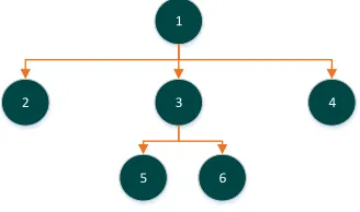
Branch-and-Bound algorithms One of the first exact solution methods for the VRP in the literature is the branch-and-bound (BB) algorithm. The BB algorithm gives an exact solution by searching in the complete solution space. The idea of the algorithm is to partition the solution space in disjunctive partitions, and then again partition the disjunctive partitions until the best feasible solution is found. The partitions can be visualized in a search tree, see Figure 3.1.

1

2 3 4

[image:33.595.218.382.331.428.2]

6 5

Figure 3.1: Example of a search tree

The branches in a branch and bound represent a possible solution. Each branch contains an upper and lower bound. These bounds can be used to discard other partitions that cannot produce a better solution. Christofides and Eilon (1969) developed one of the first algorithms that uses a branch-and-bound algorithm. Their solution method branches on arcs. The arcs can either be included or excluded in the solution. Later, Christofides (1976) developed a new way of branching: instead of branching on the arcs, he branched on the routes. That resulted in a wider but less deep search tree. Neither of these algorithms is capable of handling large instances. To handle some larger instances with the use of BB, new methods were developed that were able to derive sharp lower bounds. Christofides et al. (1981) were the first that successfully solved instances with 10 ≤ 𝑛 ≤ 25 using their lower bounds. Later, Fisher (1994) found a new way of determining a lower

bound that is able to solve several real problem instances with 25 ≤ 𝑛 ≤ 71.

(34)

26 Connexxion plane helps to tighten the linear programming relaxations. The cutting plane tightens the inequalities until a feasible solution is found (Belenguer et al. 2011, Coelho and Laporte 2013).

Dynamic programming Dynamic programming (DP) is another exact optimization approach that is capable of dealing with complex problems. DP solves the problem by dividing the complete problem into a number of problems. Then all the problems are solved until there are no more options left to create sub-problems, this is the last stage of the DP in which the optimal solution is found. Eilon et al. (1971) provide a DP formulation for a VRP. Their formulation is as follows. Let 𝑐(𝑆) be the optimal cost of a single vehicle

route through the vertices of 𝑆 ⊆ 𝒱\{0}. The objective is to minimize (3.1) over all feasible partitions {𝑆₁, … , 𝑆𝑚} of 𝒱\{0]. Let 𝑓𝑣(𝒰) be the least cost achievable using 𝑣 vehicles and delivering to 𝒰 ⊆ 𝒱\{0}.

Where 𝒰 is a subset of 𝒱\{0}. The mathematical formulations is the following:

min

𝑆_𝑟∈𝑆∑ 𝑐(𝑆𝑟) 𝑚

𝑟=1 (3.1)

𝑓𝑣(𝒰) = {

𝑐(𝒰), 𝑘 = 1 min

𝒰∗_{⊆𝒰⊆𝒱\{0}}{𝑓𝑣−1(𝒰\𝒰

∗_{) + 𝑐(𝒰}∗_{)} , 𝑘 > 1} (3.2)

In all the stages, the partial solutions are extended with an extra node. The total number of stages is equal to the number of nodes that are formulated in the DP. The stages can have a various number of states, which are partial solutions that contribute to solve the main problem. The solution cost is 𝑓𝑚(𝒱\{0}) and the optimal

partition corresponds to the optimized subsets in the recurrent formula (3.2). Christofides et al. (1981) created a DP that could handle instances with 10 ≤ 𝑛 ≤ 25. In the last few years the number of article using

DP is significantly reduced, Laporte (2009) and Kok et al. (2010) are one of the latest authors using this technique.

Commodity flow formulations A recent formulation that solves the VRP with the use of commodity flow formulation (CFF) is given by Baldacci et al. (2004). Their formulation is based on Finke et al. (1984) and is suitable for capacitated vehicle routing problem (CVRP): variable 𝑥𝑖𝑗 defines the load carried on arc (𝑖, 𝑗), an

extended graph 𝐺 = (𝒱, ℰ), where ℰ represents edges (undirected, and with symmetric distances), obtained

from 𝐺 by adding node 𝑛 + 1, which is a copy of depot node 0. Given a vertex set 𝒱 = 𝒱 ∪ {𝑛 + 1}, and

edges ℰ = ℰ ∪ {{𝑖, 𝑛 + 1}, 𝑖 ∈ 𝒱}. A vehicle route is represented by a path from node 0 to node 𝑛 + 1 in 𝐺.

Let 𝑦𝑖𝑗 be a binary variable that has value 1 if edge {𝑖, 𝑗} ∈ ℰ is in the solution and 0 otherwise. This formulation

uses two flow variables 𝑥𝑖𝑗 and 𝑥𝑗𝑖 to represent an edge {𝑖, 𝑗} ∈ ℰ of a feasible solution for the CVRP. If the

vehicle travels from 𝑖 to 𝑗, then the flow is represented by 𝑥𝑖𝑗, and the available empty space is represented

by 𝑥𝑗𝑖.

It is reported that randomly generated instances with 30 ≤ 𝑛 ≤ 60 with 𝑚 = 3 or 𝑚 = 5 are solved.

For larger instances the method becomes more inconsistently but it was able to solve up some instances with

(35)

M.H. Matena 27

Set partitioning Balinski and Quandt (1964) where the first to use a set partition (SP) formulation for the VRP with capacity restrictions, also known as the CVRP with an inhomogeneous vehicle fleet. The definition of SP is that all the feasibility is implicitly considered by the definition of the route set ℛ. A drawback of SP is that it

cannot solve nontrivial CVRP instances, due to the large number of possible routes. Despite of the drawback, SP is part of two of the most successful VRP algorithms from Fukasawa et al. (2006) and Baldacci et al. (2008)

Classic Heuristics

Classic heuristics can be subdivided into two main categories, construction and improvement heuristics. The main difference between these categories is that the construction heuristics, a feasible solution is built by adding routes from “scratch”, whereas the improvement heuristic, also known as local-search, starts with any feasible solution, which the heuristic tries to improve. The improvement heuristic, consists of two subcategories, intra- and inter-route moves. Intra-route moves improves each route separately, while with inter-routes moves of customers, the moves are analysed between different routes. It is possible that a heuristic uses both methods. We briefly discuss the heuristics mentioned by Laporte (2009): cluster-first route-second, the savings algorithm, the set partitioning heuristic (SPH), K-opt, and b-cyclic k-transfer scheme.

Cluster-first, route-second heuristics A cluster-first, route-second (CFRS) heuristic consist of two phases, namely clustering and routing. Fisher and Jaikumar (1981) formulated one of the famous CFRS heuristics, they first locate 𝑚 seeds and construct a cluster for each seed. The assignment of each customers to a cluster is solved by the generalized assignment problem (GAP). Some procedures for selecting the seeds are described by Bramel and Simchi-Levi (1995), and Baker and Sheasby (1999). The second phase in the CFRS heuristic is solving the TSP for each cluster. The savings algorithm and the set partitioning are examples of a CFRS, both are treated in the next two paragraphs.

The savings algorithm, probably the best-known heuristic for the VRP, is described by Clarke and Wright (1964). This heuristic starts with an initial (possibly infeasible) solution made up of 𝑛 back-and-forth routes (0, 𝑖, 0)(𝑖 = 1,2, … , 𝑛) where 0 represents the depot. The heuristic then evaluates all possible options to

remove arcs (𝑖, 0) and (0, 𝑗) and add arc (𝑖, 𝑗) followed by a calculation of the savings 𝑠𝑖𝑗= 𝑐𝑖0+ 𝑐0𝑗− 𝑐𝑖𝑗,

these savings are calculated for all possibilities and the insertion that yields the largest savings is implemented. The heuristic iterates until there are no more possibilities for insertions. The heuristic is easy and it can handle extra restrictions with ease, which is probably the reason why this heuristic is still popular. Golden et al. (1977) proposed an improvement by multiplying 𝑐𝑖𝑗 by a positive weight 𝜆, the route shape parameter that helps

finding the shortest route. Another improvement is proposed by Altinel and Öncan (2005), they added the customers’ demands impact while calculating the savings. They formulated the savings as follows:

𝑠𝑖𝑗 = 𝑐𝑖0+ 𝑐𝑜𝑗− 𝜆𝑐𝑖𝑗+ 𝜇|𝑐0𝑖− 𝑐𝑗0| + 𝑣

𝑑𝑖+ 𝑑𝑗

𝑑

(36)

28 Connexxion The savings parameters are explained as follows: 𝑑𝑖 is the demand of customer 𝑖, 𝑑𝑗 is the demand of

customer j, 𝑑 is the average demand of all customers, 𝜇 exploits the asymmetry information between customers 𝑖 and 𝑗, and 𝑣 is a non-negative parameter. The last part of (3.3) gives a placement priority to customers with larger demands. This improvement makes the heuristic faster and more accurate. Nevertheless this heuristic for solving the VRP, is still highly time consuming and is outperformed in time by all other heuristics described in this section.

Set Partition Heuristic (SPH), also known as “Petal Heuristic”, is another well-known set of construction heuristics. An SPH normally assumes that the vertices are distributed on a plane. The most elementary version of a Petal Heuristic is the sweep algorithm of Gillett and Miller (1974). The sweep algorithm starts with a half-line rooted at the depot, then it rotates counter clockwise or clockwise, the customers are incorporated in increasing order of the angle. The cluster stops when the load/capacity is exceeded, in which the route returns to the depot. This algorithm does not allow intersecting routes (See Figure 3.2 for a simplified case). Other SPH do allow the intersecting of routes Ryan et al. (1993).

D

Start

Figure 3.2: Example of the sweep algorithm. Start at 12 o’clock with a capacity of four customers.

K-opt The 𝑘-opt heuristic is an intra-route improvement heuristic. Croes (1958) was the first describing a type of 𝑘-opt, the 2-opt. The 2-opt method generates a 2-optimal route, which is a route that cannot be improved

by exchanging any two arcs. To accomplish a 2-opt, all the arcs that cross each other must be removed, since crossing of arcs is never optimal in the classical VRP with no capacity restrictions and a symmetric cost matrix. The 2-opt method is generalized to 𝑘-opt by Lin and Kernighan (1973). The 𝑘-opt move, changes a tour by replacing 𝑘 edges from the tour by 𝑘 other edges of the same tour, in such a way that a shorter tour is

achieved.

b-cyclic, k-transfer scheme Thompson and Psaraftis (1993) formulated an inter-route improvement heuristic,

𝑏-cyclic, 𝑘-transfer scheme, wherein 𝑏 routes are considered for relocation and 𝑘 vertices from each route,

are moved to the next route of in 𝑏. Computational results shows that combinations of variables 𝑏 = 2 or 𝑏

(37)

M.H. Matena 29

Metaheuristics

Over the last years various metaheuristics have been designed. All the current formulated metaheuristics allow the exploration of the solution space beyond the local minima. The classic heuristics can give a local minimum as result. Metaheuristics are formulated in such a way that they allow infeasible of inferior solutions to escape from local minima. Roughly all metaheuristics can be classified into three categories: local search, population search, and learning mechanisms. First we start with the local search metaheuristic, then population’s search, to end with learning mechanisms.

Local search Local search (LS) methods start with an initial solution that might be infeasible. The methods explore the neighbourhood of the current solution and moves in each iteration to a solution in that neighbourhood. A various number of methods are defined in this category to explore the neighbourhood. According to Laporte (2009) the following LS methods are used often, tabu search (Glover 1986), simulated annealing (Kirkpatrick and Vecchi 1983, Černý 1985), and variable neighbourhood search (Mladenović and Hansen 1997). These LS methods are respectively described below.

Tabu search methods are using a memory function that keeps track of the properties of the previously visited solutions, to make sure that some solutions are not considered anymore for a certain number of iterations, the so called tabu-list. In each iteration the best solution in the neighborhood is selected and written to the tabu list. The tabu list is necessary to prevent the search from cycling. To apply the tabu method to the VRP, the metaheuristic TABUROUTE is formulated by Gendreau et al. (1994). The TABUROUTE works as follows: a solution is a set 𝒮 of 𝑚 routes 𝑅1, … , 𝑅𝑚 where 𝑚 ∈ [1, 𝑀], 𝑣𝑖∈ 𝑅𝑟 if 𝑣𝑖 is a component of 𝑅𝑟, (𝑣𝑖, 𝑣𝑗) ∈

𝑅𝑟 if 𝑣𝑖 and 𝑣𝑗 are two consecutive vertices of 𝑅𝑟, and each vertex 𝑣𝑖(𝑖 ≥ 1) belongs to exactly one route.

These routes may be (in)feasible with respect to the capacity and length constraints.

F1(𝑆) = ∑ ∑𝑟 (𝑣𝑖,𝑣𝑗)∈𝑅𝑟𝑐𝑖𝑗 (3.4)

F2(𝑆) = 𝐹1(𝑆) + 𝛼 ∑ [(∑𝑟 𝑣𝑖∈𝑅𝑟𝑞𝑖) − 𝑄] +

+ 𝛽 ∑ [(∑𝑟 (𝑣𝑖,𝑣𝑗)∈𝑅𝑟𝑐𝑖𝑗+∑𝑣𝑖∈𝑅𝑟𝛿𝑖) − 𝐿] (3.5)

Where [𝑥]+_{= max (0, 𝑥)}_and_{𝛼, 𝛽}_{are two positive parameters. If the solution is feasible,}_𝐹

1(𝑆) and 𝐹2(𝑆)

coincide. 𝐹2(𝑆) incorporates two penalty terms for capacity and route duration. The TABUROUTE procedure

is as follows: a neighbour solutions consists of removing a route 𝑅𝑗 with 𝐼 ≤ 𝑗 ≤ 𝑚 of solutions set 𝒮, the

current route, and the reinsertion of 𝑅𝑚 into another solution set 𝒮′. Then the route 𝑅𝑚 is declared tabu.

Since intermediate infeasible solutions are allowed it is possible to escape from local minima.

Simulated annealing (SA) is a generic method to find an approximation for the global optimum. This method was independently presented by Kirkpatrick and Vecchi (1983) and Černý (1985). They were inspired by the statistical thermodynamics in a process called annealing in metallurgy, a technique that heats and cools steel in a controlled way to increase the size of its crystals and reduce their defects. SA works as follows, first select a random solution 𝑠 from the neighbourhood 𝑁(𝑠𝑡) of the current solution 𝑠𝑡 at iteration 𝑡. At each