The boundedly rational user equilibrium : a parametric optimization approach

(1)

The Boundedly Rational User Equilibrium:

A Parametric Optimization Approach

Oskar Eikenbroek

(2)

(3)

Title The Boundedly Rational User Equilibrium: A Parametric Optimization Approach

Master Thesis

Date October 14, 2016

Author Oskar A.L. Eikenbroek

Civil Engineering & Management, Applied Mathematics University of Twente

[email protected]

Committee Prof. dr. ir. E.C. van Berkum Centre for Transport Studies

Dr. W. Kern

Discrete Mathematics and Mathematical Programming

Dr. G.J. Still

Prof. dr. J.L. Hurink

Dr. J.C.W. van Ommeren Stochastics Operations Research

M.A. van Essen MSc.

(4)

(5)

Abstract

(6)

(7)

Summary

Ex-ante evaluation of measures in transportation systems requires accurate prediction of the choice behavior of travelers. Traffic assignment models often presume perfect ratio-nality in route choice decision making: travelers are assumed to be selfish, fully informed and can perfectly assess the consequence of choosing an alternative. In fact, any change in the system leads to a new user equilibrium in which no traveler can unilaterally change routes and improve his travel time. However, empirical studies suggest that this equilib-rium does not arise in practice. Consequently, real-world application of measures founded under perfect rationality conditions may show undesirable results.

We develop an assignment model which adopts a more realistic behavioral perspective on decision making. We adopt the notion of bounded rationality from Mahmassani and Chang (1987) in which users switch routes when the new path significantly improves travel time. Under bounded rationality, the response to an intervention of an authority is subject to uncertainty. In contrast to the user equilibrium, a range of possible responses exists and it is unknown which boundedly rational user equilibrium (BRUE) is most likely to be realized in practice.

In the Network Design Problem we need to make assumptions on the response of travelers but this may lead to adverse effects. For instance, a pricing scheme, based on the assumption that the best-performing BRUE with respect to travel time will be realized, may lead to inferior performance in the worst-performing BRUE. We therefore consider the extremes of possible network performances under bounded rationality: an indication what a policy could achieve under uncertainty.

The mathematical problem to find the best-performing BRUE flow is a program with complementarity constraints. Current approaches in literature require complex and com-putationally expensive algorithms to find solutions and guarantee neither local nor global optimality. So, these approaches are due to their complexity less appropriate for ap-plication on large networks. Our approach assesses performance in large networks and maintains limited computation times.

(8)

easy to solve. In other words, we study the behavior of the optimization problem under perturbations in the indifference band.

Whereas the best-performing BRUE problem is a difficult program, we offer a new approach that replaces the difficult constraints by easier ones. We develop an equivalent bilevel optimization problem in which the leader of the problem chooses its decision vari-ables so that the BRUE in the lower-level problem has minimum travel time (Best-case BRUE). Although the lower-level program is a convex optimization problem, the bilevel problem itself is difficult since it does not satisfy a regularity condition.

The parametric analysis shows that the feasible set and optimal value function of the lower-level problem behave continuously with respect to perturbations in the indifference band. However, the upper-level problem does not have these favorable properties and a small perturbation in the indifference band may lead to a substantial difference in flow on an arbitrary link. Intuitively, the indifference band should be a perfectly-calibrated parameter.

We offer a regularized approach, since the unfavorable properties of the Best-case BRUE lead to difficulties in calculating the flow. This approach perturbs the objective function of the lower-level problem. The corresponding problem approximates the Best-case BRUE flow distribution and the feasible set and optimal value function of this problem are continuous with respect to perturbations in the indifference band. Moreover, this refor-mulation allows us to construct a descent method to approximate a Best-case BRUE flow distribution. This approach solely uses convex and linear programs and any optimization tool can thus be used. Furthermore, we offer a relaxation approach that solves a sequence of nonlinear programs to find a Best-case BRUE flow distribution.

(9)

Samenvatting

Ex-ante evaluatie van maatregelen in verkeerssystemen vraagt om accurate voorspellingen van het keuzegedrag van reizigers. Huidige verkeersdistributie-modellen nemen aan dat gebruikers perfect rationeel zijn: reizigers zijn zelfzuchtig, volledig ge¨ınformeerd en in staat de consequenties van elk alternatief perfect in te schatten. Onder deze aannames leidt elke verandering in een network tot een gebruikersevenwicht waarin geen reziger zijn reistijd kan verbeteren door unilateraal van route te veranderen. Empirische studies laten echter zien dat een gebruikersenwicht in niet in de praktijk voorkomt. Als gevolg hiervan zijn maatregelen, ontworpen onder de aannames van perfecte rationaliteit, minder effectief in de praktijk.

Wij ontwikkelen een verkeersdistributie-model met een realistisch perspectief op rou-tekeuze gedrag van reizigers. We gebruiken de notie van beperkte rationaliteit van Mah-massani and Chang (1987) waarbij wordt aangenomen dat gebruikers alleen van route veranderen indien er een route beschikbaar is met significant minder reistijd. Onder de aannames van dit gedrag wordt de reactie op een interventie onzeker. In tegenstelling tot het gebruikersevenwicht, zorgt elke interventie voor een verzameling van mogelijke reacties en het is onduidelijk welkeboundedly rational user equilibrium (BRUE) verkeersstroom in werkelijkheid wordt gerealiseerd.

In het Netwerk-Ontwerp-Probleem moeten we echter aannames doen over de lower-level reactie. De aanname kan in de praktijk leiden tot negatieve effecten. Een tolschema, optimaal onder de aannames van perfecte rationaliteit, kan bijvoorbeeld tot een hogere totale reistijd leiden. We stellen dan ook voor om naar de uitersten van alle mogelijke BRUE verkeersdistributies te kijken. Dit geeft, ondanks de onzekerheid, een indicatie wat een interventie kan bereiken.

(10)

De scriptie laat zien dat het vaak beschouwde gebruikersevenwicht en systeem optimum speciale gevallen van de BRUE verkeersdistributie zijn. Aangezien de mathematische programma’s van het gebruikersevenwicht en het systeem optimum gemakkelijk op te lossen zijn, gebruiken we de technieken van parametrische optimalisatie in het analyseren van de best-presterende BRUE verkeersstroom.

Omdat het vinden van de best-presterende BRUE distributie correspondeert met een moeilijk optimalisatieprobleem, vervangen we de moeilijke condities door een makkelij-ker te bestuderen probleem. In het resulterende bilevel probleem kiest de leider in het

upper-level zijn variabelen zodanig dat in het lower-level het BRUE wordt gerealiseerd die voor de minste totale reistijd zorgt. Ondanks dat het lower-level programma een con-vex optimalisatieprobleem is, is het bilevel probleem een programma dat niet aan een regulariteitsconditie voldoet.

De parametrische analyse toont dat het toegelaten gebied en de optimale waarde functie van het lower-level probleem zich continu gedragen onder verstoringen in de parameter. Echter, het upper-level probleem kent deze eigenschappen niet. Een kleine verstoring in de onverschilligheidsband kan leiden tot een substantieel verschil in de vervoersstroom op een wegvak. Intu¨ıtief houdt dit in dat de onverschilligheidsband parameter perfect gecalibreerd moet worden.

De genoemde eigenschappen leiden tot problemen in het berekenen van BRUE ver-voersstromen. Wij introduceren daarom een geregulariseerd problem. Dit probleem kent een kleine verstoring toe aan de doelfunctioe van het lower-level probleem. Daarmee benaderen wat het mathematische optimalisatieprobleem van de best-presterende BRUE distributie. Het toegelaten gebied, optimale waarde function en oplossingsset van het ge¨ıntroduceerde programma gedragen zich wel continu onder verstoringen in de parame-ter. Deze aanpak geeft de mogelijkheid om eendescent methode toe te passen. De methode gebruikt louter convexe en lineaire optimalisatieproblemen om de best-presterende BRUE vervoersstroom te benaderen. Willekeurige optimalisatiesoftware kan dus worden gebruikt om de vervoersstrom te benaderen. Daarnaast introduceren we ook nog een relaxatie me-thode die het best-presterende BRUE benadert door een reeks niet-lineaire programma’s op te lossen.

(11)

Preface

I would like to acknowledge those who made this thesis possible.

My deepest gratitude goes to Georg Still. Georg, thank you for the interesting discussions, your valuable contributions and all pleasant meetings. I could not have wished for a more inspiring supervisor.

I would like to thank my supervisors Walter Kern and Eric van Berkum. Walter, I admire your eye for detail. Eric, I am grateful for your support and guidance throughout my research.

To my family and to Mani, thank you for everything.

(12)

(13)

Introduction

Transport authorities and traffic engineers encounter challenges to limit delays in trans-portation networks since these delays lead to economic wealth losses and may affect the quality of life. A wide variety of policy measures have been taken to limit congestion. Expanding infrastructure, by adding lanes or road construction, seems to be the most straightforward and popular measure. Nevertheless, road capacity expansion might lead to inferior performance of the system as a whole as illustrated by Braess et al. (2005). This

Braess’ paradox holds in practice (e.g. in Manhattan, as was shown by Kolata (1990)) and perfectly illustrates the need for policy instrument appraisal: authorities need to assess whether transport measures achieve the desired outcomes (van Wee et al., 2013).

The Network Design Problem (NDP) determines network settings so that the trans-portation system behaves optimally. It evaluates a set of measures with respect to global performance and takes into account the expected behavioral response of individuals to interventions (Brands, 2015). The NDP is frequently modeled as a bilevel optimization problem (Farahani et al., 2013). The upper level represents the behavior of a government or road authority, while the lower level represents the behavior of travelers. The authority has a certain objective to achieve (e.g. minimizing total delay) and has for this purpose the opportunity to impose measures on the network. Implementation of a policy induces a response of travelers which is expressed in a network state (distribution of traffic flow over the network) and from that the system objective is derived (Brands and van Berkum, 2014).

(18)

perform exhaustive searches over all possible decisions and then pick the best” (Conlisk, 1996, p. 675). Under these assumptions, any change in network settings leads to a new

Wardrop oruser equilibrium: a network state in which no traveler (marginally) benefits by unilaterally switching routes.

Wardrop’s first principle has major computational benefits in the static traffic assign-ment. The corresponding optimization problem, defined by Beckmann et al. (1956), is convex and under mild assumptions the existence and uniqueness of the equilibrium link flow in the traffic network is guaranteed. Any upper-level measure leads to a unique be-havioral response and uniquely determines the performance of the system. The bilevel problem implicitly assumes that the realized flows in practice are well approximated by the Wardrop equilibrium flows of the traffic assignment since we choose those network settings which turn out to be optimal in the NDP (Ban et al., 2009).

However, empirical studies show that the economic assumptions of Wardrop are debat-able. Consequently, a user equilibrium does not necessarily arise in practice. For instance, only 34% (Zhu and Levinson, 2010) to 75% (Thomas and Tutert, 2008) of all travelers follow the shortest time path. In addition, network changes turn out to be irreversible: while initial network settings are re-obtained by revoking a change, the initial traffic state is not (Guo and Liu, 2011). These findings illustrate that the evaluation of network set-tings under Wardrop’s condition is naive. Real-world application of policy interventions designed under Wardrop’s condition are not necessarily effective and may show undesir-able results. Hence, we need a more realistic and thus behavioral perspective on route choice decision making in traffic assignment models.

Bounded Rationality

We incorporate a realistic view on decision making in the static traffic assignment and adopt the notion of bounded rationality. Bounded rationality presumes decision mak-ers to be limited in knowledge and computational capacity since a decision situation is complex (Simon, 1955, 1997). In the context of route choice decision making, boundedly rational travelers make suboptimal choices due to limited awareness or the existence of thresholds (Chorus and Timmermans, 2009). In other words, travelers choose a fast - but not necessarily the fastest - route. This notion of bounded rationality in route choice was introduced by Mahmassani and Chang (1987) and explained 90% of the trips in the study of Zhu and Levinson (2010).

(19)

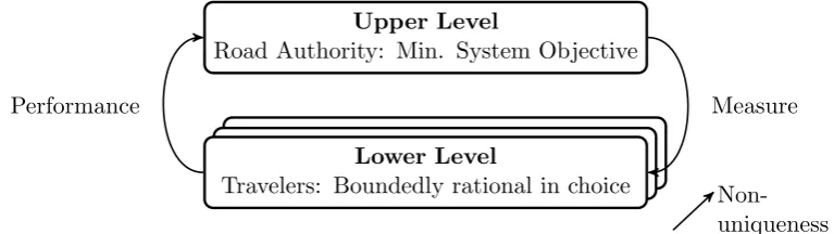
(Ban et al., 2009). The non-unique response to an intervention induces uncertainty among upper-level performances and adds a new dimension to the bilevel optimization problem (Figure 1.0.1). Whereas it is not known which lower-level flow is most likely to be realized in practice (cf. Ban et al. (2009)), it is unclear which upper-level measure optimizes the system objective.

Lower-Level Lower-Level Upper Level

Road Authority: Min. System Objective

Lower Level

Travelers: Boundedly rational in choice

Measure Performance

[image:19.595.112.496.182.290.2]

Non-uniqueness Figure 1.0.1: Network Design Problem as a bilevel problem. Adapted from Brands (2015).

Since authorities generally evaluate a (large) set of alternative measures and scenarios on large network instances, we need an efficient approach to find traffic flows as result of boundedly rational route choice behavior, as also stressed by Sun et al. (2015). Therefore we have to cope with the uncertainty in the lower-level response. In literature, it is suggested to apply the policy measure which shows (1) best worst-case performance with respect to the global objective, (2) optimal best-case performance, or (3) best performance assuming a probability distribution over all possible solutions (Ban et al., 2009; Di and Liu, 2016). Similar as in Lou et al. (2010), we consider the extremes of possible network performances under bounded rationality: an indication what a policy could achieve under uncertainty.

(20)

co-exist. The attached complex and computationally expensive algorithms to approach local minima suggest that the mentioned attempts are less appropriate for larger networks.

Based on our analysis, we make the following observations:

• The NDP requires accurate predictions of travel behavior to determine the opti-mal network settings. The conventional model presumes perfect rationality in route choice decision making and lacks empirical validity. Consequently, real-world appli-cation of measures founded under perfect rationality conditions may show undesir-able results. Empirical studies suggest that integration of bounded rationality in the traffic assignment problem increases validity of the NDP;

• Adoption of bounded rationality in the lower level of the NDP adds a new dimension to the design problem. We evaluate the extremes of the possible network perfor-mances under bounded rationality to assess performance of a measure. However, the corresponding optimization program is a complementarity constraint problem which is non-convex and there are limited approaches available to handle this diffi-cult program;

• Current approaches in literature require complex and computationally expensive al-gorithms to find the BRUE flow distributions. So, these methods are less appropriate to apply in the NDP. Moreover, since authorities evaluate a set of possible scenarios, we require an algorithm that approaches BRUE flows in limited computation time.

Research Objective

The behavioral response of travelers mainly determines the effect of a policy measure on network performance. However, current traffic assignment models make naive economic assumptions on users’ decision making processes. Assignment models should adopt a realistic view on decision making to better predict the expected outcomes of measures in the NDP. The notion of bounded rationality in route choice has the potential to predict the behavioral response of users.

This leads to the following research objective:

Development and analysis of a static traffic assignment model that incorporates

bounded rationality: travelers only switch routes when a path significantly

im-proves travel time.

(21)

Our research contributes to literature since we offer an in-depth mathematical analysis of the structure (topology) of the best and worst-performing BRUE flow with respect to travel time (Best-/Worst-case BRUE). To support our study, we add an intuitive analysis of this problem under affine linear latencies. We identify the main difficulties of the adop-tion of bounded raadop-tional choice behavior in the NDP by numerous examples. In addiadop-tion, we overcome the current complex algorithms. Indeed, we propose two algorithms that both approach the Best-case BRUE flow distribution in limited time. These algorithms allow incorporation of boundedly rational choice behavior in the NDP. We theoretically and numerically compare the proposed assignment model to the approaches of Di et al. (2013) and Lou et al. (2010).

Our theoretical analysis is necessary if we want to integrate boundedly rational be-havior in the static traffic assignment for large network instances. Moreover, the analysis supports future development of algorithms that efficiently find bounded rational link flow solutions.

Approach

This research takes a sensitivity or continuity analysis point of view. This type of analysis evaluates whether for instance the optimal value function and link flows change smoothly as the parameter changes. We provide a sufficient condition for the continuity of the fea-sible set and optimal value function of the best-case boundedly rational traffic assignment problem. We reformulate the problem as a bilevel optimization problem. In particular, we study continuity of the feasible set, optimal value function and optimal link flow solution set with respect to perturbations in the indifference band parameter for the Best-case BRUE. We approach the indifference band as a parameter since the problem of finding BRUE flows reduces for certain values of the indifference band to an easy to solve problem. This study relates to the recent paper of Di et al. (2016). Di et al. (2016) studied the continuity of the feasible set and optimal value function of the second-best toll pricing problem in a linear latency context. However, Di et al. (2013, 2016) assumed that the used route choice set is known by sequentially solving a complementarity constraint program beforehand. This assumption has serious consequences for large network instances and, therefore, we refrain from making such an assumption in our study. Han et al. (2015) investigated mathematical properties of the bounded rational dynamic assignment. Al-though the results presented can be particularly applied to the static assignment, the study mainly focused on boundedly rational flow distributions in the selection of departure times and routes. Our study, however, aims to find the BRUE flow which minimizes the total travel time in a static context.

(22)

rational route choice results from a dynamic, day-to-day, process (e.g. a repetitive choice which becomes habitual), we neither investigate these processes (see e.g. Guo and Liu (2011)) nor make any assumptions on the cognitive processes which led to a possibly suboptimal choice (see e.g. Vreeswijk et al. (2013b)). In other words, we focus on the outcomes of boundedly rational route choice behavior rather than the decision making process itself.

Outline

(23)

Chapter 2

Modeling Bounded Rationality

The economic assumptions of Wardrop state that users are able to maximize their utility function (i.e. minimize their own travel time). Users sequentially consider all possible routes and the consequences of choosing the alternative. Mathematically, we model this behavior as follows. Let Ω be the set of route alternatives for an individual and lets be the disutility function corresponding to the paths,s: Ω→R. Abstractly, the problem for each user to find alternative which maximizes utility is then:

min

x∈Ωs(x). (2.0.1)

In other words, find pointx? _∈_{Ω so that} _s₍_x_{) has its minimum at}_s₍_x?_):

x? = arg min

x∈Ω

s(x).

The assumption of bounded rationality in decision making relaxes the economic principles of Wardrop. Basically, there exist two perspectives to model bounded rationality in route choice. The first conceptualization assumes users to have limited awareness, while the second conceptualization says that the existence of indifference bands or thresholds makes that users consciously violate Wardrop’s first principle (Chorus and Timmermans, 2009). As mentioned, the first perspective assumes users to subconsciously violate Wardrop’s principle due to limited awareness: travelers do not choose the shortest path since they either do not know it is fastest or do not perceive it as such (Chorus and Timmermans, 2009; Di et al., 2013). In modeling, this perspective maintains the utility maximization behavior of users but either (i) imposes additional constraints on the set of alternatives or (ii) perturbs the characteristics of the alternatives (Hato and Asakura, 2000; Mallard, 2012).

(24)

but the set of alternatives Ω remains. The optimization problem (2.0.1) becomes

min

x∈Ωs˜(x).

Hato and Asakura (2000) imposed additional constraints on the choice set and endowed every street in a transportation network with a probability that it is observed. A chosen route only consists of links which are perceived by the user (themental map). Zhang and Yang (2015) assigned a probability to the paths in the network since users tend to choose familiar routes. The latter studies define ˜Ω ⊂ Ω as the observed set of alternatives and every agent seeks for point ˜x∈Ω so that˜

˜

x= arg min

x∈_Ω˜

s(x).

The second conceptualization assumes agents to consciously violate Wardrop’s first principle because of the existence of indifference bands or thresholds. Users are then

satisficers (Simon, 1997), solely inclined to change their itinerary when a significant travel time improvement can be achieved (Mahmassani and Chang, 1987). Travelers may possess full information on (all) the alternatives but are not necessarily utility maximizers. In this approach, users try to find point ¯x∈Ω so that

min

x∈Ωs(x) +≥s(¯x) (2.0.2)

holds. Here, >0 represents the indifference band or threshold. This conceptualization was introduced by Mahmassani and Chang (1987) and later formalized by Di et al. (2013) and Lou et al. (2010). In these static traffic assignment studies, travelers are assumed to make a suboptimal choice, i.e. the chosen route is said to be acceptable as long as the corresponding disutility is at mostworse than the alternative having minimum disutility (Lou et al., 2010). Zhao and Huang (2016) assumed the aspiration level minx∈Ωs(x) +

to be fixed: users consider any alternative which meets this level. In a day-to-day setting, condition (2.0.2) assumes users to repeat their route choice as long as an alternative cannot improve travel time more than (Wu et al., 2013).

2.1 Bounded Rationality in a

2 ×

2 -game

(25)

Player 2

L R

 

 

Player

1

T 2,2 0,1 B 1,1 3,3

Here, strategy (T, R) leads to payoff-vector (0,1): a payoff of 0 for Player 1 and a payoff of 1 for Player 2. Each player chooses to play a pure strategy or picks each strategy with a certain probability. Central in this game and in non-cooperative games in general is the notion of best reply. A selfish player chooses the strategy which maximizes utility, given the knowledge about his available strategies and the strategies chosen by the others (Peters, 2008). We restrict ourselves for the sake of clarity to this easy problem and use a graphical solution method to find allequilibria under different notions of bounded rationality. In this context, an equilibrium refers to a state in which no player has the incentive to unilaterally change strategies, i.e. there is noforce that tries to get the game in another state.

This section limits itself to some basic examples and relies on the recent elaborate literature study from Di and Liu (2016).

0 0.2 0.4 0.6 0.8 1 0

0.2 0.4 0.6 0.8 1

p

q

(a) Perfectly Rational Equlibrium.

0 0.2 0.4 0.6 0.8 1 0

0.2 0.4 0.6 0.8 1

p

q

[image:25.595.326.489.411.573.2]

(b)Limited awareness equilibrium.

Figure 2.1.1: Equilibria in 2×2-game.

Perfectly Rational Equilibrium

(26)

the other hand, leads to a payoff of 1. We have two pure equilibria in this game: (T, L) and (B, R).

More generally, assume Player 2 plays (q,1−q), i.e. he chooses L with probability q andR with probability 1−q. The best replyβ1(q,1−q) of Player 1 is to play strategyT

as long as

2q > q+ 3(1−q), or q > 3 4, holds. In other words, Player 1 will use strategyT ifq > 3

4. In case q < 3

4 Player 1 uses

B as best reply. The player isindifferent among strategiesT andB ifq = 3₄. Henceforth, any strategy combination (p,1−p), where 0≤p≤1, of T and B is the best reply. That is (Peters, 2008):

β1(q,1−q) =

        

{(1,0)} if 3₄ < q≤1;

{(p,1−p) |0≤p≤1} ifq = 3 4;

{(0,1)} if 0≤q < 3₄.

Analogously, we find β2(p,1−p) as the best reply of Player 2 against (p,1−p):

β2(p,1−p) =

        

{(1,0)} if 2₃ < p≤1;

{(q,1−q) |0≤q≤1} ifp= 2 3;

{(0,1)} if 0≤p < 2₃.

Figure 2.1.1a draws both curves: the solid line is the best reply curve of Player 1 and the dotted line is the best reply curve of Player 2. We find points of intersection. These three points are all Perfectly Rational Equilibria: ((0,1),(0,1)),((2

3, 1 3),(

3 4,

1 4)) and

((1,0),(1,0)). At such an equilibrium no player can unilaterally change strategies and im-prove utility. As we will see later, this definition is similar to the definition of a Wardrop equilibrium oruser equilibrium in the static traffic assignment.

Limited Awareness

The conceptualization of limited awareness assumes players to subconsciously violate the perfect rationality condition since travelers either do not know all strategies or the utility function is perturbed. We start with the latter approach and introduce noise to account for the perception error of a player. Let us assume that Player 2 uses strategy (q,1−q) and that Player 1 has a certain probabilityPT of playing strategyT. The probabilityPT

equals the probability that the utilityUT of strategyT is greater than or equal to utility

UB corresponding to playing B:

(27)

Following Ben-Akiva and Lerman (1985), the utility is divided into a deterministic and random part:

PT =P r(2q+ηT ≥q+ 3(1−q) +ηB).

We assume that the random variablesηT,ηB are independently and identically distributed

and are Gumbel-distributed with scale parameter µ. The probability that Player 1 will playT in response to strategy (q,1−q) is then (we omit the calculus, see Ben-Akiva and Lerman (1985)):

PT =

eµ(2q)

eµ(2q)₊_eµ(q+3(1−q)).

This results in the best reply sets for both players:

β1(q,1−q) = {(p,1−p) |p= e

µ(2q)

eµ(2q)₊_eµ(q+3(1−q))} for 0≤q≤1,

β2(p,1−p) = {(q,1−q) |q= e

µ(2p+1−p)

eµ(2p+1−p)₊_eµ(p+3(1−p))} for 0≤p≤1.

Again, Figure 2.1.1b plots the curves and we find the point of intersection (assumingµ= 1) numerically. We find a single equilibrium, known as thequantal response equilibrium (Di and Liu, 2016) or, in a traffic assignment setting, as the stochastic user equilibrium (Sheffi, 1985). Here, no traveler thinks that a switch in routes improves the travel time. Intuitively, µis the rationality parameter: if µ= 0 users are perfectly rational whileµ→ ∞ assumes users to be completely indifferent (i.e. the probability PT is independent of utilities UT

and UB).

Another approach to model limited awareness in a game is by imposing additional constraints. For instance, using the approach of Hato and Asakura (2000), we assign a probability forobserving strategyT. Player 1 is solely aware that strategyT can be played in, say, 1

4 of the cases. In the other cases, he can only playB. In 1

4 of the cases a perfectly

rational equilibrium arises since we assume that players maintain utility maximization in decision making. With probability 1₄, the best reply functionβ1(q,1−q) becomes:

β1(q,1−q) ={(0,1)|if 0≤q≤1}.

Let us assume that the set of best replies for Player 2 remains. Figure 2.1.2a plots both curves and we find the equilibrium at ((0,1),(0,1)). Observe that with probability 3

4 the

best reply function is as in Figure 2.1.1a.

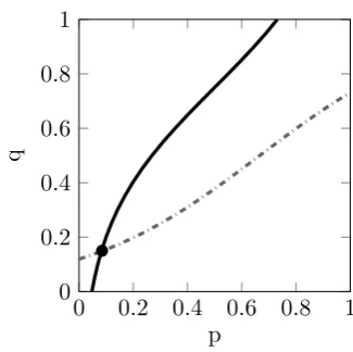
-Equilibrium

(28)

0 0.2 0.4 0.6 0.8 1 0

0.2 0.4 0.6 0.8 1

p

q

(a) Limited awareness equlibrium.

0 0.2 0.4 0.6 0.8 1 0

0.2 0.4 0.6 0.8 1

p

q

[image:28.595.135.507.83.267.2]

(b)-Equilibrium.

Figure 2.1.2: Equilibria in 2×2-game assuming bounded rationality.

by at least. Recall the earlier example. Assume Player 2 uses strategy (q,1−q). Player 1 solely plays strategy T if strategyT gives at leasthigher utility thanB:

2q > q+ 3(1−q) +, or q > 3 + 4 .

Player 1 plays (1,0) as reply if q > 3+₄. Similarly, the player solely usesB ifq < 3−₄ and is indifferent between T and B (any strategy will do) if 3−

4 ≤q≤ 3+

4 . We use the set of

sufficing replies to find all-Equilibria:

β1(q,1−q) =

        

{(1,0)} if 3+

4 < q≤1;

{(p,1−p) |0≤p≤1} if 3−₄ ≤q≤ 3+₄;

{(0,1)} if 0≤q < 3−

4 .

In a similar way, we findβ2(p,1−p) as the reply of Player 2 against (p,1−p):

β2(p,1−p) =

        

{(1,0)} if 2+₃ < p≤1;

{(q,1−q) |0≤q≤1} if 2−

3 ≤p≤ 2+

3 ;

{(0,1)} if 0≤p < 2−₃.

This notion is similar to the notion of the BRUE used by Mahmassani and Chang (1987) in the static traffic assignment. In the traffic assignment, individuals try to find a satisfactory route rather than the optimal one. In this setting we find a set of possible solutions assuming= 1₂ (Figure 2.1.2b): ((0,1),(0,1)),((1,0),(1,0)) and ((p,1−p),(q,1−q)|3−

(29)

2.2 Bounded Rationality in Route Choice

Common practice is to model route choice behavior by a perfectly rational equilibrium. As mentioned, this equilibrium lacks empirical validity but is easy to calculate. We compare the outcome of this equilibrium with the limited awareness equilibrium in Figure 2.1.1a and Figure 2.1.1b. We see that the analysis of a single scenario under different behavioral assumptions may lead to completely different outcomes in terms of link flows and travel time. Consequently, the severity of congestion on certain links (i.e. bottlenecks) is possibly different and we may derive other optimal settings from the NDP.

In the remainder of this study we adopt the notion of the -equilibrium, also called BRUE in our context. Major benefit of this notion is that we study policy implications under realistic behavioral assumptions and do not need to make any assumptions on the cognitive processes of traffic users. By this we mean that we model the outcome of users’ decision making by deriving the indifference bandfrom observed choice behavior without the necessity to study the perceptions of travelers. The other discussed approaches all require a set of rules to derive the choice strategy.

A large body of empirical studies confirms that chosen routes deviate from the fastest one. Zhu and Levinson (2010) found that only 35% of the trips were made via the shortest time path, while 90% of all trips could be explained by an indifference band of 5 minutes. A small GPS study from Jan et al. (2000) revealed an average indifference band of 0.6 minutes with respect to shortest travel time path. The fastest route was only traveled by 31 of the 124 trips. The analysis of Ciscal-Terry et al. (2016), recording 89 drivers over a period of 17 months, indicated that the observed average travel time was on average 4 minutes more than the shortest time path, including a bias due to setup and finishing operations of the driver. Although the width of the indifference band is not of interest here, the mentioned studies empirically support the incorporation of the BRUE in the traffic assignment.

From a mathematical perspective, Figure 2.1.2b illustrates that the boundedly rational user equilibrium comes with more complexity: for >0, there exist an infinite number of equilibria.

2.3 Synthesis

(30)

(31)

Chapter 3

Formal Problem Description

3.1 Notation & Traffic Assignment Formulation

We study the static traffic assignment. Given is a directed traffic network G = (V, E), with V being the set of nodes and E is the set of directed edges (road, links, or arcs) e = (i, j), where i, j ∈ V. The network includes a set of origin-destination pairs (OD pairs)K ⊆V ×V, with static demand dk>0, k∈ K. We refer to each OD pair k∈ K as

commodity kand each OD pair is connected by a set of simple directed paths, denoted by

P_k. The set P of all paths in the network is the union of the path sets per commodity:

P =∪_k∈KPk.

A feasibletraffic flow orflowfor given demandd∈R|K|+ (we denote by|.|the cardinality

of a set) is a pair of vectors (f, x)∈_R|P|_×

R|E|= (fp, p∈ P;xe, e∈E) so that

x= Γf, Λf =d, and f ≥0. (3.1.1)

Here, the matrix Γ∈_R|E|×|P| _{denotes the} _{link-path incidence matrix} _{in which Γ}

ep = 1 if

edgeeis in routep and Γep = 0 otherwise. Λ∈R|K|×|P|is the OD-path incidence matrix; Λkp = 1 ifp∈ Pkand Λkp = 0 otherwise. The conditions in (3.1.1) say that (i) the flow on

a link equals the sum of all path flows that pass through this link (i.e. (f, x) is consistent), (ii) the sum of flows on all paths for a commodity meet the demand, and (iii) path flows (and thus link flows) are non-negative.

Each link e∈ E in the network has a flow dependent travel time orcost le(x). The

travel timec(f) c:R|P|+ →R

|P|

+

along a route is additive. In other words, the cost of a route cp(f), p∈ P, is the sum of travel costs on all edges in that path:

cp(f) =

X

e∈p

le(x) or c(f) = ΓTl(x) = ΓTl(Γf)

(32)

We assume that the travel time of a trip is the only determinant in route choice. Furthermore, in choosing routes, travelers are assumed to value travel time homoge-neously. Literature refers to these settings as the fixed demand static traffic assignment

ornonatomic routing game.

Assumption 1. Let us assume throughout the study that the travel time function l(x) is separable (i.e. le(x) =le(xe)), continuous, convex and strictly monotone: le(xe)< le(¯xe)

providedxe<x¯e.

We emphasize that Assumption 1 is not necessarily a very strong one and applies to general travel cost functions, including the well-known BPR-function (Bureau of Public Roads) or a - more general - polynomial with positive coefficients.

3.2 Wardrop’s Principles

Wardrop (1952) formulated two alternative criteria to determine the distribution of flow over a traffic network. The first principle was formulated as: “the journey times on all the routes actually used are equal and less than those which would be experienced by a single

vehicle on any unused route” (Wardrop, 1952, p. 345). Wardrop’s first principle assumes travelers to be perfectly rational in making route choice decisions: users maximize own utility by considering and evaluating all possible alternatives. The resulting traffic flow pattern (fn_{, x}n_{) (the superscript} _n _{refers to John F. Nash, who introduced the perfectly}

rational equilibrium in non-cooperative games) under the assumptions of this behavior in a static environment is a traffic state in which no traveler can unilaterally change routes to decrease its own travel time.

Definition 3.2.1 (PRUE). Consider a traffic flow(fn_{, x}n₎_{as in (3.1.1) with}

correspond-ing cost vector c(fn₎_{. Flow} ₍_fn_{, x}n₎ _{is said to be a Perfectly Rational User Equilibrium}

(PRUE) if for allk∈ K the following condition holds for allp, q∈ P_k:

f_pn>0⇒

  

cp(fn) =cq(fn) if fqn>0;

cp(fn)≤cq(fn) if fqn= 0.

(3.2.1)

In particular, at PRUE as in (3.2.1) all flow-carrying paths (i.e. p ∈ P :fn

p > 0) for a

commodityk∈ K experience equal (in fact, minimum) cost minq∈Pkcq(f

n_).

Beckmann et al. (1956) formulated an optimization problem to a PRUE flow distribu-tion:

min

(f,x)z(x) s.t. (f, x) as in (3.1.1), (Qn)

where

z(x) :=X

e∈E

Z xe

0

(33)

(fn_{, x}n_{) solves (}_Q

n) under Assumption 1 if and only if this flow satisfies the

Karush-Kuhn-Tucker (KKT) conditions corresponding to (Qn) (note that the feasible set is defined by

linear (in)equalities and the objective function z(x) is strictly convex). The system of KKT conditions with corresponding multipliers (µ, φ, λ) for this problem reads, assuming l(x) to be continuously differentiable, as follows:

∇_xs(x)−µ = 0 ΓT_µ₋_ΛT_λ₊_φ _{= 0}

fT_φ _{= 0}

(Γf −x)T_µ _{= 0}

(d−Λf)T_λ _{= 0}

φ ≥0 f ≥0 d = Λf Γf =x

(3.2.2)

Since ∇xs(x) =l(x), the system (3.2.2) corresponding to (Qn) reveals that flow-carrying

paths share (minimum) travel cost as in (3.2.1). Indeed, simple analysis shows that λk

represents the minimum cost to travel for commodityk∈ K. We obtain, where the travel time on the minimum cost path for commodity k∈ K is denoted by λn

k, that traffic flow

(fn_{, x}n_{) as in (3.1.1) is a PRUE flow if and only if}

f_pn(cp(xn)−λnk) = 0, and cp(xn)≥λnk (3.2.3)

is satisfied for allp∈ P_k, k∈ K. The system defined by (3.1.1) and (3.2.3) is thenonlinear complementarity problem (NCP) for finding the PRUE flow distribution.

Note that since the objective function z(x) in problem (Qn) is strictly convex on the

feasible set defined by the (in)equalities in (3.1.1), a PRUE (fn_{, x}n_{) exists and is unique}

with respect toxn _(and _λn_).

Remark 3.2.1 (Non-unique route flows). As widely discussed in literature, there may exist a set of route flows f corresponding to a single link flow distribution x (see Lu and

Nie (2010)). Let us regard the setH(x) of route flows for known link flowx of pair(f, x)

(and fixed d) as:

H(x) ={f ∈_R|P| | Λf =d,Γf =x, f ≥0}.

Solely under the condition that the matrix

"

Λ Γ

#

has full column rank there is only a

sin-gle route flow solution f corresponding to link flow x. With exception from parallel-link

networks, we cannot expect that this condition is satisfied in general.

(34)

Formally, a flow (fs_{, x}s_{), superscript} _s _{referring to system optimum, as in (3.1.1) is}

said to be a system-optimal traffic flow if the flow minimizes total travel time. In other words, (fs_{, x}s_{) solves the following optimization problem:}

min

(f,x)s(x) s.t. (f, x) as in (3.1.1), (Qs)

where

s(x) =X

e∈E

xele(xe). (3.2.4)

Under Assumption 1, the objective function s(x) - representing total travel time - is (strictly) convex. Then, (fs_{, x}s_{) solves (}_Q

s) if and only if (fs, xs) satisfies the KKT

conditions of (Qs) with corresponding Lagrange multiplier vectors. These conditions are

similar to (3.2.2) with the only difference that ∇xs(x) = l(x) +xT∇xl(x). This reveals

that the resulting traffic flow is a PRUE flow using marginal cost ∂

∂xe(xele(xe)) as latency function for each link e∈E. Equivalent to the PRUE condition in (3.2.1), a traffic flow (fs_{, x}s_{) as in (3.1.1) is a system optimum if and only if}

f_ps>0⇒

  

˜

cp(xs) = ˜cq(xs) iffqs>0;

˜

cp(xs)≤˜cq(xs) iffqs= 0,

(3.2.5)

is satisfied for allp∈ Pk, k∈ K, where

˜ cp(x) :=

X

e∈p

le(xe) +xele0(xe)

,

and l0

e(xe) = ∂l_∂xe(_ex).

Again, the objective functions(x) of (Qs) is strictly convex on the feasible set defined

by the (in)equalities in (3.1.1) and the system-optimal traffic flow distribution (fs_{, x}s₎

exists and is unique with respect toxs_.

3.3 Synthesis

(35)

Chapter 4

Boundedly Rational User

Equilibrium

4.1 Formal Definition

The assumptions of perfect rationality in route choice decision making are, from a behav-ioral perspective, naive. The boundedly rational equilibrium condition in (4.1.1) states that travelers are satisficers so that unilaterally switching routes cannot lead to a travel time improvement of more than an individually-tailored and situation-specific tolerance threshold: the indifference band (Mahmassani and Chang, 1987; Vreeswijk et al., 2013a). Although this behavior might be in practice the result of limited awareness, our modeling perspective assumes travelers to be fully informed.

Definition 4.1.1 (BRUE). Given the indifference band ∈_R|K|₊ , a traffic flow (f, x) as in (3.1.1) with corresponding path costs c(f) is called a Boundedly Rational User Equilib-rium (BRUE) if for all k∈ K the following condition is satisfied for all p∈ P_k:

fp >0⇒cp(f)≤ min

q∈P_kcq(f) +k. (4.1.1)

BRUE condition (4.1.1) was first articulated by Mahmassani and Chang (1987), and was, among others, formalized by Di et al. (2013) and Lou et al. (2010). Condition (4.1.1) formulates a range of allowable travel times for a user by introducing indifference band or

tolerance vector ∈R|K|+ . This is clearly in contrast to PRUE condition (3.2.1) that only

contains a single value of allowed travel times for each OD pair: minq∈Pkcq(f), k ∈ K. Consequently, the BRUE flow distribution (i.e. satisfies (4.1.1) is a traffic state in which the travel time of any flow-carrying path is within the formulated range. A BRUE flow may possess the property that all minimum cost paths carry no flow (assuming >0). In the remainder, we call a path p ∈ Pk, k ∈ K, acceptable if cp(f) ≤ minq∈P_kcq(f) +k is

(36)

We assume that the indifference bandk, k∈ K, in (4.1.1) is exogenous, i.e. the range

of acceptable travel times is independent of traffic state (f, x). Moreover, we assume that k does not differ among users of the same commodity k ∈ K. These assumptions

might not reflect real-world situations. For example, some travelers might be oblivious in their route choice with respect to congestion (they choose their route with respect to shortest distance) while others, more frequent users, choose routes based on previous ex-perienced delays. This behavior can easily be incorporated by introducing heterogeneous users (adding a superscript on user type dependent variables and parameters) or by ap-proaching the indifference band as a random variable. An endogenous tolerance vector (f), i.e. is a function of f, as in Han et al. (2015), might be more appropriate in a dynamic setting.

Remark 4.1.1 (Multiplicative indifference band). It remains an open question whether it is preferable to incorporate an additive (as in condition (4.1.1)) or multiplicative

in-difference band with respect to the minimum cost path (see Christodoulou et al. (2011),

Roughgarden and Tardos (2002)):

fp >0⇒cp(f)≤ min

q∈P_kcq(f)(1 +k). (4.1.2)

Empirical studies do not (yet) answer this question. From a mathematical analysis point of

view the condition in (4.1.1) has major advantages. We will highlight results (see Remark

6.3.1 and Remark 6.4.1) in the remainder of this study in which the analysis does not hold

under assumptions of a multiplicative indifference band as in (4.1.2).

4.2 Illustrative Examples

In previous sections, we discussed the differences in modeling route choice decision mak-ing based on perfectly rational and boundedly rational choice behavior. In this section, illustrative examples show the implications using BRUE rather than PRUE in the NDP.

Given a network instance, the PRUE link flow distributionxn_{is uniquely determined.}

So the corresponding system’s objective value s(xn_{) is uniquely determined as well. Let}

us show that under BRUE condition (4.1.1) uncertainty among performances with respect tos(x) and x arises.

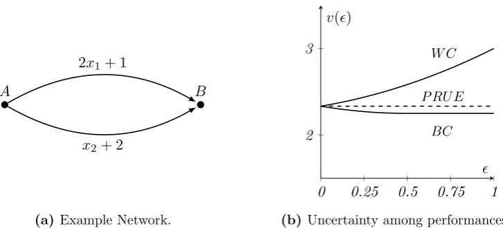
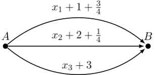
Example 4.2.1 (Uncertainty among performances). Consider the two-link network in Figure 4.2.1a. Both paths (1,2) connect commodity (A, B) and are endowed with a strictly monotone linear latency function. We send demandd= 1 from node A toB.

The PRUE link flow distribution xn _{(see condition (3.2.1)) is uniquely determined:}

xn=

2 3,

1 3

(37)

2x1+ 1

x2+ 2

A B

(a) Example Network.

0 0.25 0.5 0.75 1

2

3 _{W C}

P RU E

BC

v()

[image:37.595.124.488.86.251.2]

(b)Uncertainty among performances.

Figure 4.2.1: Network and performance results for Example 4.2.1. (BC = Best-case, WC = Worst-case.)

Given ≥ 0 we have a set of link flows satisfying (4.1.1). This set of feasible flows is denoted by F() and given by

F() =n (x1,(1−x1)) 2−₃ ≤x1 ≤ 2+₃, 0≤x1≤1

o

.

As discussed, non-uniqueness of BRUE flow distributions may lead to difficulties in

deter-mining performance of a certain measure. Let us consider the best and worst-performing

BRUE with respect to total travel time for a given≥0. Hence, for any≥0we find the flows that satisfy (4.1.1) and minimizes and maximizes s(x) respectively.

Figure 4.2.1b plots the total travel time v() in both cases for each ∈ [0,1] in . We show that performance may differ significantly. Further, we make the observation that the

Best- and Worst-case BRUE provide a lower and upper bound respectively for the total

travel time under Wardrop’s first principle (i.e. s(xn₎_{). Note that for}_{= 0} _{both the}

Best-and Worst-case BRUE reduces to the PRUE flowxn_.

We interpret Example 4.2.1 as follows. Compared to the PRUE, the BRUE flow distribution is not necessarily unique. In the NDP, any upper-level policy instrument leads to a set of BRUE flows among which performance may differ substantially. If the lower level of the NDP adapts the PRUE condition (3.2.1), a naive measure - optimal under this condition - might be implemented. Indeed, in the next example we show that policy interventions designed under Wardrop’s first principle might lead to an inferior performing Worst-case BRUE. Basically, Example 4.2.2 illustrates that if we use bounded rationality in the static traffic assignment, then we should base or tolling scheme on the BRUE assignment as well.

(38)

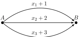
x1+ 1

x2+ 2

x3+ 3

[image:38.595.244.398.90.161.2]

A B

Figure 4.2.2: Network in Example 4.2.2.

for an overview). Assume we have the possibility to set (time-independent) tolls τ on all

edges in the network.

0 0.25 0.5 0.75 1 2

W C

BC

v()

(a) Best- and Worst-case performance with no tolls.

0 0.25 0.5 0.75 1 2

W C

BC

v()

[image:38.595.143.496.252.415.2]

(b) Performance with tolls.

Figure 4.2.3: Performance results for Example 4.2.2. (BC = Best-case, WC = Worst-case.)

We look at the simple parallel-link network (three paths connect commodity (A, B)) (Figure 4.2.2). Based on Beckmann’s minimization problem (Qn) and the system optimum

(Qs) we arrive at the PRUE and system-optimal flow distribution xn, xs, respectively:

xn= (1,0,0), xs=

3 4,

1 4,0

.

We derive the first-best pricing strategy: a toll pricing strategy that allows all links to be

tolled with any toll. Recall that we have for a system-optimal flow (fs_{, x}s_{) the equilibrium}

KKT condition

X

e∈p

le(xse) +xsel

0

e(xse)≥λks, for allp∈ Pk, k∈ K.

Note that such a flow distribution will not occur under perfect rationality conditions since

individuals then only consider le(xe) and not l0e(xe)xe (i.e. the impact of their choice on

others). The first-best tolling strategy easily follows from previous equation if the disutility

(39)

toll vector τ ≥0 that satisfies the following conditions leads to a system optimum under perfectly rational decision making (Yang and Huang, 2005):

le(xse) +τe≥min e∈E(le(x

s

e) +xse),

X

e∈E

(le(xse) +τe)xse=dmin e∈E(le(x

s

e) +xse).

So, a first-best tolling scheme would be to impose τe=xsel0e(xse) =xse for all e∈E. Figure

4.2.4 depicts the link cost functions including the tolls.

x1+ 1 + 3₄

x2+ 2 + 1₄

x3+ 3

[image:39.595.228.382.220.294.2]

A B

Figure 4.2.4: Latency functions with tolls for Example 4.2.2 .

Suppose in practice a BRUE flow, ≥ 0, is realized. We show again the Best- and Worst-case performing BRUE (with and without the induced toll) and compare global

per-formance in Figure 4.2.3a and Figure 4.2.3b.

The results in Figure 4.2.3b show that the first-best tolling scheme always induces a

system optimum if we assume that the Best-case BRUE is realized. This follows from the

observation in Example 4.2.1: the Best-case BRUE performs at least as good as the PRUE

and since the PRUE reduces to a system optimum, the Best-case BRUE reduces to this

global optimum as well.

However, for certain values of ≥ 0, edge 3 becomes acceptable (i.e. travel time on this edge is within from the shortest). This was not taken into account in the first-best

tolling scheme since xs

3 =xn3 = 0. In the Worst-case BRUE, path3 might be utilized and

therefore worsens overall performance of the network.

Example 4.2.2 supports our earlier claim that the toll scheme should be adapted to its behavioral assumptions. It might be suggested that an authority induces a toll after observing flows in a transport network: the naive PRUE flow distribution will not arise in practice. However, a PRUE flow is also a BRUE traffic flow and thus the PRUE distribution might be observed after all. Example 4.2.2 shows that the Worst-case BRUE performance with the tolls might be worse compared to the Worst-case BRUE without tolls. We suggest that a pricing scheme which minimizes Worst-case BRUE performance is more appropriate in this setting.

(40)

In practice, not only link flow x is of importance, but route flow f as well. For instance, relieving a bottleneck by giving pre-trip route advice requires that the link flow is disentangled by commodities. As widely discussed, there may exist several route flows f that correspond to a single link flowx (Lu and Nie, 2010). An arbitrary route flow f corresponding tox(e.g. as by-product of a convex combination method in the PRUE) may lead to several difficulties. First, in a PRUE, it may cause discontinuity inf with respect to perturbations; a small change in the demand leads, from a behavioral perspective, to completely different route choice behavior (Lu and Nie, 2010). Second, several route flow distributions corresponding to the same x are incomparable (Borchers et al., 2015). Again, let us regard the setH(x) of route flows for known link flow distributionxof BRUE solution (f, x, λ) (and fixed d) as a point-to-set mapping:

H(x) =nf ∈R|P| |Λf =d,Γf =x, f ≥0

o

.

It is desirable to have a signle realistic route flow and therefore we impose additional conditions on f. Conventional methods in literature use a two-stage approach to derive PRUE route flow fn _{out of} _xn _{(e.g. by maximizing entropy). That is: first calculate}

link flow x and, independently, use x to find f. We indicate that additional difficulties arise under bounded rationality compared to perfect rationality. If we choose f ∈ H(x) arbitrarily this may not only lead to discontinuous and incomparable route flows in a PRUE setting, it may also generate route flows which are infeasible under BRUE condition (4.1.1) (see Example 4.2.3 below).

3x1+ 3

4x2+ 4

6x3+ 2

6x4+ 3

6x5+ 4

A

B

[image:40.595.229.411.468.554.2]

C D

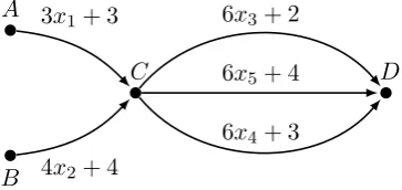
Figure 4.2.5: Considered network in Example 4.2.3.

Example 4.2.3 (Determining f out of x). Consider the network in Figure 4.2.5. Assume there are two commodities (A, D) and (B, D), both with demand 1.We have six path flows: f13, f14, f15, f23, f24, f25. Given link flow x, route flow f is not uniquely

determined since

rank

"

Λ Γ

#

(41)

Suppose (A,D) = 2 and (B,D)= 1. A BRUE link flow is:

x= (x1, x2, x3, x4, x5) =

1,1,2 3, 2 3, 2 3 ,

and the corresponding path cost vector c(x):

c(x) = (c13(x), c14(x), c15(x), c23(x), c24(x), c25(x)) = (12,13,14,14,15,16).

Choose two route flows f1_{, f}2_{∈ H}₍_x₎_:

f1 = (f₁₃1 , f₁₄1 , f₁₅1, f₂₃1 , f₂₄1 , f₂₅1) =

1 3, 1 3, 1 3, 1 3, 1 3, 1 3 ,

f2=

0,1 3, 2 3, 2 3, 1 3,0

.

In case f1 _{is the resulting route flow, the flow is infeasible since} _c

25(x)−c23(x) = 2 >

(B,D) = 1. However, if we choose f2, f252 = 0 and all paths that carry flow are in the

range of acceptable travel times:

˜

f25 c25(x)−c23(x)−(B,D)

= 0.

We interpret Example 4.2.3 as follows. The choice of route flowsf ∈ H(x) for a BRUE flowxinfluences theexperienced travel time. Givenf1_{, f}2 _{∈ H}₍_x_{) and both correspond to}

BRUE link flow distributionx(as in the example). The example shows that the maximum travel time among all flow-carrying paths differs forf1_and_f2_{. Indeed, for}_f1_{the maximum}

travel time for commodity (B, D) is 16 while the maximum travel time underf2 _{is 15.}

All in all, given BRUE flow x, not all f ∈ H(x) are feasible BRUE route flows. More-over, if we want to give route advice to relieve a bottleneck, the choice off corresponding tox influences the travel time for travelers.

From a mathematical perspective, this conclusion is trivial since the problem adds additional conditions compared to the problem to find the PRUE flow. Later we will see that the non-uniqueness of route flows plays an essential role in the continuity of the feasible set and optimal value function of the Best-case BRUE flow distribution.

Remark 4.2.1. We note that the issue of infeasible route flows f ∈ H(x) does not occur in a PRUE and system-optimal setting. Nonetheless, in a system optimum (and any

other flow not in PRUE), the choice of route flow f corresponding to x influences the

experienced travel time. In a system-optimal traffic assignment, travelers are assumed to

be memoryless: the choice of a bypass at a node is independent of the travel time up to

(42)

4.3 BRUE in Other Settings

BRUE flow distributions also appear in other settings. The first analogy concerns system-optimal route guidance in traffic networks with user constraints, the second setting de-scribes a more general matrix game.

Route Guidance with User Constraints

Opposed to individual performance, road authorities are in general concerned with the per-formance of the transport system as a whole. It is well-studied that individual and system interests in this context may interfere: an individual optimum may lead to a degradation of the transport system as a whole (Roughgarden, 2005). The system-optimal traffic flow distribution (fs_{, x}s_{) is known to require cooperation among travelers or complete}

coordi-nation of the authority in all route choice (Yang and Huang, 2005). A possible measure to achieve this system-optimal traffic assignment is by means of route guidance systems.

Current navigation systems, however, provide descriptive or advisory information and guide travelers in a self-interest way based on shortest instantaneous travel times. As mentioned, this may lead to an inferior performance of the system. A traffic routing strategy that aims for a system optimum diverts some individuals to significantly longer routes to minimize global performance (Jahn et al., 2005). As a result, these drivers may not comply with such advices and the optimal state will not be achieved, i.e. in a system-optimal assignment unfairness or inequity among individuals arises.

For our purpose, let us define unfairness ηk(f) for traffic flow (f, x) as the maximum

difference in travel time between a used route and the cost the fastest alternative for commodityk∈ K:

ηk(f) = max

cp(f)−minq∈Pkcq(f) fp>0, p∈ Pk

. (4.3.1)

We show in the next proposition that a system optimum suffers under unfairness issues, earlier presented for a single commodity in Correa et al. (2007). In particular, if we consider the BPR-function, in a system-optimal route guidance some travelers end up traveling 5 times as long as others. Note that ηk(fn) = 0 for all k ∈ K where (fn, xn)

satisfies (3.2.1)

Proposition 4.3.1. (Correa et al., 2007). Suppose δ ∈_N is the maximum degree of the polynomial of the link cost function l(x) used in the network. Given that (fs_{, x}s₎ _solves

(Qs) then

ηk(fs)≤(δ+ 1) min q∈Pk

X

e∈q

le(xes)

(43)

Proof. The proof is similar to the proof in Correa et al. (2007). It is shown by Roughgar-den (2002) that under Assumption 1,le(xe) +xel0e(xe)≤(δ+ 1)le(xe) for alle∈E and for

all xe≥0. For instance, for monomials (i.e. le(xe) =xeδ), le(xe) +xel0e(xe) = (δ+ 1)xeδ.

Hence, we can upper bound the marginal cost of a path by a constant factor of the la-tency function. A lower bound on the marginal cost for a link is straightforward under Assumption 1: le(xe) +xele0(xe)≥le(xe).

Let λs

k denote the minimum marginal cost for commodity k ∈ K for system-optimal

traffic flow (fs_{, x}s_{). Recall that all flow-carrying paths experience these marginal cost}

(3.2.5). Pick p ∈ Pk, k ∈ K so that fp >0 and take q ∈ Pk as a minimum latency path

for commodityk∈ K, we arrive at:

λs_k =X

e∈p

le(xse) +xesl0e(xes)≥

X

e∈p

le(xes)≥

X

e∈q

le(xes),

and

λs_k≤X

e∈q

le(xse) +xesle0(xes)≤

X

e∈q

(δ+ 1)le(xes).

Hence, it turns out that the travel time is bounded by a constant factor from the travel time on the shortest path:

X

e∈p

le(xes)≤(δ+ 1) min q∈Pk

X

e∈q

le(xes).

The claim of the proposition follows directly.

van Essen et al. (2016) pointed out that users are willing to use alternatives with higher travel times as long as the difference with respect to the fastest path is found to be acceptable. Therefore, Jahn et al. (2005) proposed a system-optimal routing strategy incorporating unfairness among individuals with respect to an apriori determinednormal length. Unfairness with respect to this normal length - independent of flow - was chosen for computational purposes. We suggest that the distribution of travel time among users is a more appropriate indicator to measure unfairness.

Let us assume that the travel time differences as defined in (4.3.1) solely determines the acceptability of a route guidance system. The problem of finding a system-optimal traffic route guidance system with user constraints (i.e. every traveler uses an acceptable route) becomes:

min

(f,x)s(x) s.t.

(f, x) as in (3.1.1); ηk(f)≤k for all k∈ K.

(4.3.2)

In this problem, k ≥ 0 is the upper bound in travel time difference for commodity

(44)

flow distribution as in (4.1.1) which minimizess(x) (i.e. Best-case BRUE).

-Nash Equilibria

Game Theory often uses Nash equilibria to model the behavior of individuals in non-cooperative games (cf. Section 2.1). Here, the player’s strategy is the best reply given the other players strategy (Peters, 2008). Then, an equilibrium is a solution of a game in which no player can unilaterally change strategies and improve his or her utility (note the equivalence with PRUE condition (3.2.1)). An-(approximate) Nash equilibrium is a strategy profile in which no player can improve payoff by more than ≥0 (Nisan et al., 2007). Let us formally define this solution concept using the notation of Nisan et al. (2007).

Adopting the definition of Nash equilibrium of Nisan et al. (2007), strategy vector s∈S is said to be an-Nash equilibrium, ≥0, if for all playersi∈ {1, . . . , n} and each alternative strategys0_i∈Si, we have that

ui(si, s−i)≥ui(s0i, s−i)−. (4.3.3)

Here,si denotes the strategy played byiands−i the strategies played by all other players.

ui(si, s−i) is the utility of player i. Trivially, condition (4.3.3) reduces to the definition of

a conventional Nash equilibrium when= 0.

-Nash equilibria gained attention in behavioral game theory (incorporating experi-mental economics into strategic decision making) to efficiently approximate true Nash equilibria (Nisan et al., 2007) and in (non-)atomic routing games (Christodoulou et al., 2011). In non-atomic routing games, condition (4.3.3) reduces to (4.1.1). An interesting open problem in the latter field is upper bounding the Price of Anarchy for flows (f, x) that satisfy condition (4.1.1).

4.4 Synthesis

(45)

Chapter 5

Best-Case BRUE

Authorities concern themselves with the impact of measures on transportation systems. Lou et al. (2010) highlighted that a BRUE flow distribution is not necessarily unique and causes uncertainty among performances (see also Section 4.2). So it is important to assess performance of flow distributions with best and worst-case performance with respect to system’s objective (case BRUE). Following our discussion, the Best/Worst-case BRUE flow is a solution of the program (5.0.1).

min/max₍_f,x₎s(x) s.t. (f, x) satisfies (4.1.1) (5.0.1) In our case, the system cost functions(x) in (5.0.1) will be the total travel time (3.2.4). Nevertheless, any other objective function can be used as long as it is strictly convex with respect to link flowx. The upcoming sections particularly focus on the Best-case BRUE problem.

We emphasize that the formulation in (5.0.1) does not necessarily find the BRUE flow distribution which is most likely to be realized in practice. Some BRUE flow distributions may be unrealistic in real-world applications. Since we assume that an authority has no control over which BRUE will be realized for a given tolerance vector, we only consider the extreme cases (best, respectively worst, system performance).

5.1 Problem Definition

(46)

• We denote the n-dimensional Euclidean space and its non-negative orthant by Rn andRn+ respectively;

• TheEuclidean norm of a vectorx∈_Rn _{is defined by} _k_x_k_:= P

i=1:n|xi|2

1₂

.

• TheFrobenius norm of a matrix A= (aij)∈Rm×n is defined as kAk=k(aij)k2;

• Amultifunction or point-to-set mapping F ofX ⊆_Rn _into_Y _⊆

Rm assigns to each x∈X a (possibly empty) subset F(x) of Y;

• Thedomain of a multifunctionF consists of allx∈X for whichF(x) is nonempty: dom (F) :={x∈X |F(x)6=∅};

• Ur(A) is defined as a neighborhood of radius r ∈R+ around set A :Ur(A) :={x ∈

X | infy∈Akx−yk< r}.

The optimization problem to find the Best-case BRUE flow distribution(s) (5.0.1) is equivalently formulated as follows. We minimize total travel time while the constraints assure that the difference in travel costs between users of the same commodityk∈ Kdoes not exceed indifference bandk≥0. More precisely, the Best-case BRUE is a solution of

min

(f,x,λ)s(x) s.t. (f, x, λ)

∈ F(), (Q())

where the feasible set F() is given by

F() =

      

(f, x, λ)∈R|P|×R|E|×R|K|

(f, x)∈ F₀

(f, x, λ)∈ Fl

(f, x, λ)∈ Fu()

      

.

Here,F₀ assures that the resulting traffic flow (f, x) is feasible (i.e. (f, x) is as in (3.1.1)). Due to the linear (in)equalities,F₀ is a convex set and is formally defined to be

F₀ ={(f, x) |x= Γf,Λf =d, f ≥0}.

F_l and F_u() arise due to the bounded rationality condition (4.1.1). The setF_l is defined as

F_l={(f, x, λ) | −cp(x) +λk≤0 for all p∈ Pk, k∈ K},

and Fu(), ≥0, is defined to be

Fu() ={(f, x, λ) |fp >0⇒cp(x)−λk ≤k for allp∈ Pk, k∈ K}.

The term λk is (a lower bound on) the minimum travel cost for commodity k ∈ K.

(47)

for that commodity, while Fu() defines the travel time of a flow-carrying path to be

within the range [λk, λk +k]. Obviously, any flow (f, x) ∈ F() satisfies the BRUE

condition (4.1.1). Conversely, any (f, x) that satisfies (4.1.1) is contained in F() by taking λk = minp∈Pkcp(x) for all k ∈ K. Hence, we will refer to any point (f, x)∈ F() with correspondingλas a BRUE (flow distribution).

Consider ∈ R|K|+ as a parameter vector. Our problem (Q()) is then a parametric

optimization problem. The objective function s:R|E|→R of (Q()) is defined in (3.2.4), is independent of the parameterand is strictly convex with respect to link flowsx.

The parametric problem (Q()) assesses performance of BRUE flow distributions with best-case performance (with respect to the system cost). That is, find BRUE flow distribu-tion which minimizes travel time among all possible BRUE flows for a given indifference band . Figure 5.1.1 abstractly illustrates to process to find the Best-case BRUE: we seek for the flow distribution ( ˜f ,x˜) closest to (the unique with respect to x) (fs_{, x}s_{) with}

respect tos(x).

F() (fn_{, x}n₎

[image:47.595.133.458.358.543.2]

(fs_{, x}s₎ ( ˜f ,x˜)

Figure 5.1.1: Abstract illustration of the feasible BRUE set F(). (Q()) finds ( ˜f ,x˜) closest to (fs_{, x}s_{) with respect to}_s₍_x_).