The other margin: do minimum wages cause working hours adjustments
for low-wage workers?
Mark B Stewart & Joanna K. Swaffield
No 746
WARWICK ECONOMIC RESEARCH PAPERS
The other margin: do minimum wages cause working hours
adjustments for low-wage workers?*
Mark B. Stewart University of Warwick
&
Joanna K. Swaffield University of York
February 2006
This paper estimates the impact of the introduction of the UK minimum wage on the working hours of low-wage employees using difference-in-differences estimators. The estimates using the employer-based New Earnings Surveys indicate that the introduction of the minimum wage reduced the basic hours of low-wage workers by between 1 and 2 hours per week. The effects on total paid hours are similar (indicating negligible effects on paid overtime) and lagged effects dominate the smaller and less significant initial effects within this. Estimates using the employee-based Labour Force Surveys are typically less significant.
Keywords: Minimum wages, working hours, labour demand,
difference-in-differences estimator.
1. Introduction
The effects of minimum wages have long been debated and are the subject of fierce disagreement. Most heavily investigated has been the impact on employment, testing the hypothesis that a minimum wage reduces the demand for low-wage workers. Labour demand adjustments may also take place at the hours margin and there is rather less evidence on this impact. Potential hours adjustments are the focus of this paper.
In April 1999 the UK, following a change of government, and based on the recommendations of a report from the independent Low Pay Commission (LPC, 1998), introduced a National Minimum Wage. This followed a period without wage floors, following the abolition in 1993 of the Wages Councils that had covered certain vulnerable sectors. The minimum was introduced at an adult rate of £3.60 for all employees aged 22 and over and a youth rate of £3.00 for those aged 18 to 21. Compliance has been high. The available evidence suggests an almost complete truncation of the wage distribution at £3.60 for adult workers after April 1999 (LPC, 2001, Stewart and Swaffield, 2002, Dickens and Manning, 2004b) and little in the way of wage spillovers (Dickens and Manning, 2004a).
Existing empirical work on the impact of the introduction of the minimum wage suggests that while it may have had an adverse effect on employment in particular sectors (Machin et al, 2003, for care home workers), the overall effect on employment has been broadly neutral (Stewart 2002, 2004a, 2004b). However potential labour demand shifts caused by the minimum wage introduction may also manifest themselves as a change in employees’ hours of work. Firms may reduce employment at either or both of the extensive and intensive margins: the number of workers and/or the number of hours per worker. A full analysis of any labour demand shift resulting from the minimum wage requires an analysis of both these potential responses.
“reducing hours appears to be the most common tactic adopted by employers wishing to avoid paying the minimum wage” (New Review, Low Pay Unit, 1999). In comparison, Connolly and Gregory (2002) using the New Earnings Survey and the British Household Panel Survey found no evidence of working hours reduction for female workers directly affected by the introduction of the minimum wage. Although research in this area is relatively limited, the time-series literature suggests “hours per week fall when minimum wages increase, so the effect on hours worked is more pronounced that the effect on bodies employed” (Brown, 1999, page 2156).
The potential impact on hours is also important to the wider minimum wage debate. Michl (2000) suggests that one possible explanation for the differences between the results of Card and Krueger (1994, 2000) on the one hand and Neumark and Wascher (2000) on the other in their analyses of the impact of the New Jersey 1992 minimum wage increase on the fast-food industry may lie in their different treatment of hours worked per employee. Neumark and Wascher use total payroll hours as their dependent variable, and so would capture any hours adjustments. Card and Krueger use the number of workers as their dependent variable and so would not. Although the debate between the two sides focused largely on the quality of the data used, Card and Krueger (2000) note in their conclusions, despite their reservations about the data used by Neumark and Wascher, that “an alternative interpretation … is that the New Jersey minimum-wage increase did not reduce total employment, but it did slightly reduce the average number of hours worked per employee” (page 1419).
Other US evidence points to the importance of hours in considering the full impact of minimum wages on low-wage employees: Linneman (1982), Neumark et al (2004). Whether motivated primarily by a focus on labour demand shifts or on overall income effects for low-wage employees, there is a clear need to evaluate the impact of the minimum wage introduction on the working hours of low-wage employees.
This paper tests whether the April 1999 introduction of the UK minimum wage had a significant impact on the working hours of low-wage employees, using individual-level longitudinal data from two national datasets: the New Earnings Survey (NES) and the Labour Force Survey (LFS). The paper uses difference-in-differences estimators to estimate a model of an individual employee’s change in paid working hours (within the same job) as a function of the individual’s initial position in the wage distribution. Estimators are constructed using different definitions of the group directly affected to examine the robustness of the findings. Alternative “wage gap” and spline estimators are also presented.
The next section outlines arguments for why we might expect hours adjustments for low-wage workers directly affected by the introduction of the minimum wage. Section 3 details the estimation strategy used in the paper. Section 4 provides a brief description of the two datasets and the construction of the key variables required for the analysis. Section 5 presents results from the difference-in-differences estimation and extensions thereof. It also tests the fundamental identifying assumption underlying the difference-in-differences estimator. Section 6 presents a summary of the main findings.
2. Theoretical predictions of the effect on working hours
the number of (paid) hours per worker. In the long run a firm’s choice of workers-hours mix depends on the extent of fixed costs of employment, the technology and productivity-hours schedule, the labour supply schedule faced, the presence and effectiveness of a union, etc. However in the short run, as Hamermesh (1993) observes, “employers are quicker to alter hours in response to shocks than they are to change levels of employment” (page 294).
Further, if effort per hour worked can also be varied, workers may be made to work harder per hour to raise productivity in line with the wage, thereby reducing the overall hours required for a particular task. For current purposes, whether this increased productivity and reduction in hours arises through higher productivity levels during paid hours of work or employers requiring workers to complete designated tasks in their own (unpaid) time if not completed during paid hours is less important than the prediction of working hours reduction - a prediction in line with the competitive model when the market wage rate is raised above the equilibrium level.
However the prediction for hours worked is likely to be more complex than this, even in the context of the simple competitive model. It is a well-established stylized fact that full-time employees are paid more than otherwise similar part-time employees, which suggests that full-timers produce more per hour. If this were the case, firms would be expected to lengthen workweeks in response to a minimum wage increase rather than reduce them (Brown, 1999, page 2117). This is particularly so if hours are fixed within both the full-time and part-time groups. If however one assumes that there will be employment-hours substitution within part-time and within full-time, the tendency would again be toward fewer working hours.
When considering the likely impact on working hours of the introduction of a minimum wage in the UK a number of stylized facts concerning minimum-wage workers also seem relevant to consider. These workers tend to be relatively low skilled prior to employment and receive relatively limited training whilst in post. They also tend to have higher than average turnover rates. Both these points suggest relatively low fixed costs associated with the employment of this type of worker. Minimum wage employment also tends to be within the service sector, where the intensity of capital usage and potential substitutability of capital for labour is relatively low and the incidence of part-time employment is high. In addition, minimum wage workers tend to be from groups (for example based on race or gender) that are disadvantaged in the labour market and have low levels of union representation. Finally, UK employment law may make labour demand adjustments at the intensive margin, at least in the short to medium term, easier than at the extensive margin.
3. Estimation strategy
The construction of the two groups for comparison in the difference-in-differences estimator is of course crucial to this approach. Consider first how to construct the group of individuals directly affected by the introduction of the minimum wage (known as the “treatment” group in the methodological literature on difference-in-differences estimation). One possibility is to construct this group as those whose wage was below the level of the minimum prior to its introduction. This is the group used in the analysis of the impact on the probability of remaining in employment (Stewart, 2004a). Defining the group of those directly affected in this way ignores incomplete compliance.
When analyzing the impact on hours (unlike when looking at that on the number employed), one can also use the information on the wage at time t+1. The affected group is better defined as those individuals earning below the minimum, whose wage was actually raised to comply with the new minimum. Using the information on the wage at t+1, the group of those directly affected can be defined as those with a wage at t, prior to introduction, below the incoming minimum, and a wage at t+1, after the introduction, above the new minimum. This refinement improves the definition of the group affected by using this additional information, but also increases the extent of the exogeneity assumption required for the difference-in-differences estimator to be consistent.
The assumption of an exogenous wage requires that if there is a firm-specific shock (e.g. to the demand for its product), the firm may adjust hours or employment but is not able to adjust the wage. This strengthening of the required assumptions when the contemporaneous wage at t+1 is used suggests that it is worthwhile investigating both constructions of the “treatment” group. Results are therefore presented based on both definitions.
Ideally we would wish to compare this affected group with itself in an alternative state of the world when the minimum wage had not been introduced, which is of course not possible. The approach used here to address the counter-factual questions is to construct a second group of employees who act as the control or comparison group. If these individuals are similar enough to those affected by the minimum wage introduction, the effect of the minimum wage can be estimated by comparing the experiences of these two groups before and after the minimum wage introduction. The importance of the definition of the control group in this approach is clear. This group needs to be constructed to be similar enough to the sub-minimum-wage group directly affected by the minimum wage introduction to generate equivalent behavioural responses, but not be themselves affected by the introduction. A group with initial wages just above the minimum is used here.
The validity of the estimator requires a number of assumptions. Suppose that in the absence of a minimum wage the change in hours can be decomposed into two components, with the first component fixed over time and the second component common across groups. This assumes that in the absence of a minimum wage the difference in the average change in the hours of work between groups would be the same in each time period, or equivalently that the time paths of hours growth would be the same for each group. This important assumption will be tested in Section 5 below. Suppose further that the minimum wage has a constant effect, θ, on the change in hours of work for those in group g=1 and no effect on those in group g=2. Now consider two time periods, the first, starting at t1,where there was no minimum
wage in place at either t1 or t1+1, and a second, starting at t2, where the minimum
across these two time periods (starting t1 and t2) gives θ. Thus the raw
difference-in-differences estimate is given by double differencing these sample means.
Define hit to be the hours of work of individual i at time t. The focus here is on the
change in hours, yit = hit+1 - hit. The difference-in-differences estimator is given by:
2 1 2 1
(1) (1) (2) (2)
ˆ (yt yt ) (yt yt )
θ = − − − (1)
where ( )g t
y denotes the average of yit over i in group g.
This difference-in-differences estimator can also be generated by a linear regression using micro data pooled across groups and time periods. If binary indicator variables are included for group g=1, time period 2, and the interaction between them, then the OLS estimator of the coefficient on the interaction will be the
difference-in-differences estimator, ˆθ. This simple specification is generalized in three ways in the model used here. First it is extended to produce a “regression adjusted” difference-in-differences estimator by adding a vector of individual characteristics thought to influence changes in working hours. In adding these control variables the aim is to deal with any differences between the “affected” or “treatment” group (g = 1) and the “comparison” or “control” group (g = 2) not controlled for with the additive group and time effect dummies. Second, as indicated above, an additional group containing the rest of the wage distribution above the control group is added (with additional indicator variable). This will improve the estimation of the effects of the individual characteristics. Third multiple pre-minimum time periods are used (with additional time dummies).
Define d1i = 1(individual i is in group g=1) = 1(wit < mt+1), where 1(A) is the indicator
function, equal to 1 if A is true and equal to 0 if not, and define qt = 1(t < t* < t+1),
yit = xit′β + α1d1i + α3d3i + γ0qt + γt + θd1iqt + ϕd3iqt + εit (2)
where d3i = 1(individual i is in group g=3) = 1(wit≥ mt+1(1+c)), with the control group
(g=2, i.e. mt+1 ≤ wit < mt+1(1+c)) being the excluded base category, xit is a vector of
individual characteristics, γt are aggregate time effects, and E[εit⏐xit, g, t] = 0. In the
basic specification used in this paper the control group is defined as those employees with wages between the minimum wage and 10% above the minimum (i.e. c = 0.1).1 The sensitivity of the estimates to this choice of upper limit is investigated by also considering a wider control group and by a graphical examination. There is a trade off here. Widening the control group improves cell sizes and hence precision of estimation, but may lessen the similarity between the affected and control groups.
This specification uses the first definition of the affected or treatment group discussed above. The second definition of this group described above uses the data on the wage at t+1 in addition to that at t. The affected group now contains those with a wage below the incoming minimum at time t and above it at time t+1. The specification of the model needs to be extended slightly in this case. Since the post-minimum treatment and control groups are now restricted to those with wage at t+1 above the minimum, there is now an additional group of individuals, containing those with wage at t+1 below the minimum, i.e. those not in compliance.
The specification adopted here is to include indicator variables for this group partitioned into the three wage ranges previously identified.2 This construction of additional groups applies to the period where t+1 is after the introduction of the minimum wage. Prior to the introduction of the minimum the majority of those with a real wage at t below £3.60 do not see their real wage at t+1 rise above £3.60. However the appropriate inter-temporal comparison is with individuals at a similar
1 In the second definition of the “treatment” group, using the wage information at t+1, it is excluding
those whose wages at t+1 fell to below the minimum.
2 One might also consider using a single variable for the group as a whole, a restricted version of the
place in the wage distribution at t. It is therefore not appropriate to restrict the group in this way for the pre-minimum periods.
The specification used defines an indicator variable for those with wage at t+1 above the minimum, ait+1 = 1(wit+1≥ mt+1), and one for those below, bit+1 = 1-ait+1. The
alternative specification is therefore:
yit = xit′β + α1d1i + α3d3i + γ0qtait+1 + γt + θd1iqtait+1 + ϕd3iqtait+1 + δ1d1iqtbit+1
+ δ2d2iqtbit+1 + δ3d3iqtbit+1 + εit (3)
with θ again being the parameter of main interest.
There are two key identifying assumptions underlying the modelling processes in equations (2) and (3). The first is that the interaction effects are zero in the absence of the minimum wage, after controlling for differences in observable characteristics. The issue of concern is that even in the absence of the minimum wage introduction, change in working hours may occur differentially in different wage groups. The validity of this assumption is tested below. The second key identifying assumption is that the introduction of the minimum wage does not influence the working hours of employees in the control group (g = 2). Changes may occur to the control group due to wage spillover or substitution effects between different groups of workers. However the evidence for the UK minimum wage introduction suggests that this has not been the case.
alternative approach uses a “wage gap” variable that is the difference between the wage at time t and the minimum wage in place at time t+1 (Currie and Fallick, 1996).
This approach is equivalent to replacing d1i in equation (2) with its product with this
new “wage gap” measure. Offsetting the advantages of using this specification, a problem with the “wage gap” estimator is that it is adversely affected by any unduly low values of the wage variable. As a result, it is more vulnerable to measurement error in the wage than the “binary indicator” estimator. There is something of a discrepancy between the representations above and below the minimum in these “wage gap” specifications: the equivalent of a spline term is used below the minimum, but binary indicator variables are used above the minimum. One can go one step further by modelling the range of the wage distribution above the minimum with linear spline terms as well as that below. Estimators of this type are also presented below.
4. Data
The two data sets used in this paper are the New Earnings Survey (NES) and the Labour Force Survey (LFS). Data from the annual NES are utilised from April 1994 (after the abolition of the Wages Councils) up to April 2000. Data from the quarterly LFS are used from the first quarter of 1997 to the third quarter of 2000. The LFS can only be used from 1997 quarter 1 onwards, when earnings questions were added to the wave 1 questionnaire. Prior to this, earnings questions were only asked of the outgoing, wave 5, respondents. The LFS provides 15 quarterly waves of data, and therefore 11 matched (t to t+1) time periods a year apart. The NES provides 7 annual waves of data, and therefore 6 matched (t to t+1) time periods. The paper uses data for adult employees, defined as being aged between 22 and 59 (inclusive) for women and between 22 and 64 (inclusive) for men at time t, who were with the same employer (and in the same job) at times t and t+1.
often) directly from their computerized payroll records, and second, the very large sample size, providing much larger cell sizes for the different effects to be analysed than the LFS. The NES also has a potentially important drawback, with most employees who earn below the PAYE deduction threshold excluded from the NES. This particularly affects part-time workers. An employee earning below the minimum at time t, who has their wage increased at time t+1 to comply with the minimum wage, could potentially fall out of the sample if working hours were reduced to the extent that weekly earnings were then less than the PAYE deduction threshold. The LFS has a different problem, with some responses provided by proxy rather than by the employee in question. This increases the possibility of measurement error. Although always an issue with measures of wages and hours, this is potentially greater when the wage and hour questions are not answered directly by the employee.
For both the NES and LFS data, “initial” and “lagged” effects of the introduction of the minimum wage are estimated. The initial effects are defined over time periods where the minimum wage is introduced at some point between t and t+1. The lagged effects are defined over time periods where the minimum wage is introduced between t-1 and t. The argument for estimating these lagged effects is that if employers are constrained in their labour demand responses to the introduction of the minimum wage, either through contractual obligations or the slower implementation of the minimum wage rates, labour demand responses may not be observed immediately. Instead a lagged effect of the minimum wage introduction on the change in working hours might be expected
For the NES, the initial effect is defined in terms of the difference in working hours between April 1998 (t), when no minimum wage was in place, and April 1999 (t+1), when the minimum wage was in place, and compares this with differences entirely pre-NMW. NES lagged effects compare differences over April 1999 (t) to April 2000 (t+1) with the same pre-NMW periods.
compare the differences defined over April 1999 (so the minimum wage is in place at time t) to September 2000 with the same pre-NMW periods. For both the LFS and NES data sets the t+1 time periods used in the lagged effects are prior to the first adult uprating of the minimum wage in October 2000.
Two hours measures are analysed in both datasets: basic working hours and total paid working hours. Basic working hours are defined as the hours worked by employees as part of their standard employment contract before overtime. Total paid working hours are the sum of the basic hours and paid overtime hours. (Unpaid overtime hours are excluded.) The distinction between the two is potentially important since some employees may be able to choose to adjust overtime hours, but this is unlikely to be the case for basic hours.
For the NES the gross hourly wage variable is a “basic hourly wage rate”. It is defined as gross weekly earnings excluding overtime, divided by normal basic hours. It is restricted to employees whose pay for the survey period was not affected by absence. For the LFS the gross hourly wage variable is an “average hourly wage rate”. It is constructed as gross pay in the most recent pay period, converted to a weekly basis and then divided by usual hours per week.3 For both data sets the gross hourly
wage rate is deflated to April 1999 using the all-items RPI.
The difference-in-differences approach based on position in the wage distribution used in this paper requires that those in the directly affected group, below the minimum wage, experience larger wage growth than those in the comparison group, above the minimum, and that this difference shows up significantly in the wage measure used in the construction of these groups for the analysis of the effect on hours. That this is indeed the case is demonstrated by Stewart (2004a) for both the NES and LFS datasets used here.
3 From the spring quarter of 1999 a new question was added to the LFS questionnaire that asked
5. Results
5.1 Evidence on the fundamental identifying assumption
The fundamental identifying assumption underlying the difference-in-differences approach is that in the absence of a minimum wage the time paths of hours growth would be the same for each of the wage groups. i.e. that there are no significant interactions in the pre-minimum wage period between the wage group effects and the time effects. To formally examine whether this assumption holds for the data used in this paper we follow the procedure in Stewart (2004a) by restricting attention to the pre-minimum wage period and testing the significance of interactions between the wage group and time dummies for the period when no minimum wage was in place.
For the pre-minimum wage period in the LFS data the joint test statistic p-values with and without control variables for total paid hours were 0.25 and 0.39 for the male sample and 0.44 and 0.59 for the female sample. In each case therefore the tests provide evidence supporting the underlying assumption of no interactions. Test statistic p-values for basic hours only are even larger and hence provide even stronger evidence in favour of the underlying assumption of no interactions in the absence of the minimum wage.
For women the NES data are more supportive of the assumption. For total paid hours, test statistic p-values of 0.41 (0.21) without (with) controls provide strong evidence supporting the underlying assumption. For basic paid hours there is some evidence of a marginally significant interaction for 1997-98. However the effect is small and to allow equivalent comparisons between total and basic paid hours in the reported estimates for women the 1997-98 data were not excluded from the pre-minimum wage period. The baseline estimates presented below change little if this wave is excluded.
5.2 Graphical examination of hours changes
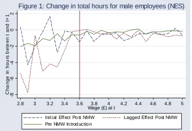
Before presenting the estimated effects on hours of work using the difference-in-differences estimator and extensions thereof, we present here a simple graphical examination of the hours changes by wage group in the NES and LFS datasets. Figure 1 shows the average change in total paid hours (basic plus paid overtime) between t and t+1 for male employees in the NES plotted against the hourly wage at time t, using cells of width 10p. Figure 2 shows the equivalent plot for women. Both figures show evidence of a negative lagged effect (and a more limited initial effect) for those initially below £3.60 per hour (in real terms adjusted to April 1999) relative both to the pre-minimum period and to those above £3.60. The plots look very similar for changes in basic hours only.
The graphs below £3.60 give some evidence that a wage gap representation might be more appropriate than a binary indicator (i.e. that hours changes are larger for lower initial wage rates). However there is a worry that low values of the wage may be distorted by measurement error which may unduly affect the wage gap estimates.
Since the sample sizes in the LFS datasets are much smaller than in the NES, the corresponding LFS plots would be based on very small cell sizes. We therefore use a moving 20p window for the LFS plots presented in Figures 3 and 4. For men there is some evidence of negative initial and lagged effects for those initially below £3.60, relative both to the pre-minimum period and to those above £3.60, but there is also more fluctuation in the plots for both of these comparators. For women there is little evidence of any differences – either between the three plots or comparing above and below £3.60. (Again the plots look very similar for changes in basic hours only.)
5.3 Difference-in-differences estimates
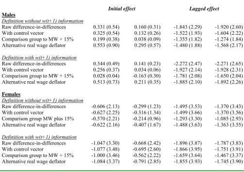
Difference-in-differences estimates of initial and lagged effects, for the NES for adult male and female employees are given in Table 1.4 For men, the raw
difference-in-differences estimate of the initial effect is insignificant for both the change in total paid hours and the change in basic hours. In comparison the lagged effect, capturing the impact after the initial period, is negative and significant for both hours measures.
The estimates with control variables included imply a lagged effect of a reduction in total paid hours of about 1.5 hours per week as a result of the introduction of the minimum wage and a total effect (initial plus lagged) of about 1.2 hours. Almost all of this effect comes through a reduction in basic hours. There is a negligible effect on paid overtime hours.
4 For the NES the control vector includes year dummies, regional dummies, age (and square), hourly
When the alternative definition of the wage groups employing also the information on the wage at (t+1) is used, the initial effects remain insignificantly different from zero. The lagged effects strengthen slightly and imply a reduction in total paid hours of about 1.9 hours per week, all through a reduction in basic hours, and a total effect (initial + lagged) of about 1.7 hours.
The construction of the comparison group is potentially crucial to the difference-in-differences estimator. Estimates are also presented in Table 1 for a comparison group constructed to include those up to 15% above the April 1999 minimum. This reduces the magnitude and significance of the lagged effect. The magnitude of the combined effect (initial + lagged) however changes relatively little. The sensitivity of the estimates to the choice of real wage deflator is shown. If this is changed from the Office for National Statistics all-items RPI to the RPI excluding mortgage payments, the results are fairly robust, although indicating a slight fall in overall magnitude and significance for the lagged effects.
The lower panel of Table 1 gives the corresponding estimates for women. All are negative. For the initial effects the estimates for total paid hours are all significantly negative, while those for basic hours are all insignificant with the first definition of the wage groups, but significant when the definition utilizing also the information on the wage at (t+1) is used. The lagged effects are negative and significant for both total and basic hours and for both wage group definitions. For women the overall (initial + lagged) effect on total paid hours is slightly larger than that for men at about 2.1 hours using the first wage group definition and about 2.9 using the second definition. The female NES estimates appear relatively robust to the inclusion of the control vector, widening of the comparison group and an alternative real wage deflator.5
5 The evidence for women in Table 1, of a reduction in hours after the introduction of the NMW, is in
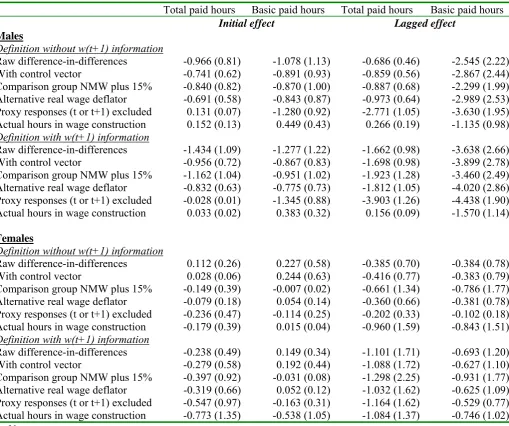
The results based on the LFS data are given in Table 2. The estimated initial effect is insignificant for both total and basic hours and for both men and women, and this finding is robust to the various modifications of specification presented. The lagged effect estimates for total paid hours are insignificant for both men and women, as are those on basic hours for women. The lagged effect on basic hours for men, however, is significantly negative and relatively large in magnitude, indicating a reduction in basic hours for the affected group relative to the comparison group, after the minimum wage introduction, of 2.9 hours with the first definition and 3.9 with the second. The significance of this estimate is similar to that of the estimates in Table 1 for men on the NES, although the magnitude of the LFS estimate is slightly larger. The difference between the estimates for basic and total hours suggests that changes in the former may have been partially offset by changes in overtime hours in this case.
As mentioned above the LFS suffers from a potential problem of additional measurement error caused by proxy responses. If observations with a proxy response at either t or t+1 are excluded from the sample, which obviously affects cell sizes, the findings are not greatly affected. For men both lagged effects become more negative, but the standard errors also rise markedly.
The sensitivity of the estimates to the construction of the hourly wage rate used to construct the wage groups is also examined in Table 2. If instead of dividing usual weekly pay by usual weekly hours to construct the average hourly wage, the actual hours of work for a specified week (not necessarily matching the pay period) are used, all four effects for women and both initial effects and the lagged effect on total paid hours for men remain insignificant. However now the lagged effect on basic hours for men also becomes insignificant and the magnitude is much reduced. Of all the sensitivity issues investigated for the LFS this is the one with the greatest impact on the estimates.
5.4 Alternative estimators using “wage gap” and spline constructions
estimates are presented in the “wage gap: dummies above” rows of Table 3. The rows below that additionally model the range of the wage distribution above the minimum with linear spline terms as well as that below the minimum. These pairs of rows provide results that are similar to each other, particularly when they are significant. Comparisons with the original NES “binary indicator” estimates show the “wage gap” specification to increase the significance of the estimates for both the initial and lagged effects for men, but only for the initial effects for women. For the LFS all “wage gap” and spline estimates were found to be insignificant. This included the previously significant lagged impact on basic hours for men.
To compare the magnitudes of the “binary indicator” and “wage gap” (and spline) estimates it is most informative to evaluate the “wage gap” impact at the average distance of the wage at time period t from the minimum wage rate at t+1. For men in the NES the average lagged impact of the minimum wage is estimated at approximately -1.7 for total paid hours (the product of the average wage gap for wage group 1 (£0.54) and the coefficient estimate (-3.08)) and -1.5 for basic hours. For women in the NES the initial effect was estimated as -0.7 for total paid hours and -0.6 for basic hours. In both these cases the magnitude of the average effect based on the “wage gap” specification was similar to the original “binary treatment” estimate. In contrast to this, the male initial “wage gap” effects are oppositely signed to the original effects, although only of marginal significance, and the female lagged average “wage gap” estimates are less than half the “binary treatment” estimated effects.6 Although the “wage gap” and spline estimators have certain advantages, it should be noted, as stated in Section 3, that they are adversely affected by unduly low values of the wage variable and hence more vulnerable to measurement error in the wage than the “binary indicator” estimator.
5.5 Further robustness checks
As with all survey data, hours variables are likely to suffer from a degree of measurement error. How this potential measurement error affects the estimates here
6 The average value of the “wage gap” variable for the NES initial (lagged) estimates was £0.62 (£0.54)
depends on the nature of the measurement error, for example whether it satisfies the assumptions of the classical model or not. Unfortunately there are no formal validation studies, for example comparing the responses of employees with those of their employers, for the hours variables on either the NES or the LFS. Evidence from the US (Duncan and Hill (1985), Mellow and Sider (1983), Bound et al (2001)) may provide some limited pointers. This suggests that employees tend to over-report hours of work compared with employers. However there is also evidence that professional and managerial workers and more educated workers are more prone to this over-reporting, suggesting that it may be less of a problem for the low-paid workers who are central to the analysis in the current paper.
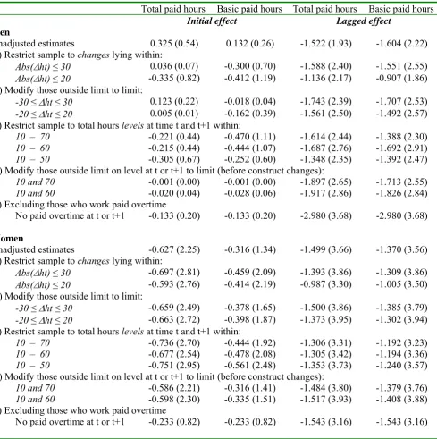
A potential concern with regard to this paper is that the estimated effects may be exaggerated because of some large changes in working hours, which might in some cases be due in part to measurement error. The approach adopted is to examine the robustness of the results to excluding various groups who might be thought to have a higher probability of measurement error in hours. Tables 4 presents NES difference-in-differences estimates for samples where observations viewed as having a higher potential for measurement error are either excluded or have their hours moderated. These exclusions or truncations of the distribution are based on either the changes in hours between t and t+1 or the underlying levels at t and t+1. It should be noted that these modifications involve an endogenous selection or censoring. They should not therefore be viewed as alternative estimates on an equal footing with the original estimates, but rather are presented to give an impression of the robustness of the unmodified estimates.
The fifth block of Table 4 excludes those who work paid overtime at either t or t+1. The reasons for looking at this last modification are two-fold. The first relates to the issue of measurement error. One might expect those who work (paid) overtime to show more variation in their hours from week to week and might expect this to increase the probability of measurement error in reported hours. A second reason concerns the interpretation of the estimated effects as demand responses. If the effects presented were supply responses, since one might expect employees who work (paid) overtime to have more scope to adjust their hours, this would lead one to expect the estimates to decline (in absolute value) when those working paid overtime are excluded. This does not happen. For women the total of initial and lagged effects increases very slightly from an estimated reduction of 1.7 hours to 1.8 hours. For men it doubles from an estimated reduction of 1.5 hours to one of 3.1 hours. Thus the original result is not being driven by the effect for those who work overtime. This mitigates against a supply interpretation. In addition the exclusion of a group more likely to be prone to measurement error, as before, does not reduce the effect.
Overall it would appear that the estimates presented in this paper, and the implied impact of the introduction of the minimum wage on the working hours of low-wage employees, are relatively robust to excluding observations that are potentially more likely to suffer from measurement error.
6. Conclusions
Lagged effects are found to dominate the initial effects. On the basis of the NES, the lagged effect on basic hours is estimated to be a reduction of between 1 and 2 hours per week. The lagged effect on total paid hours is very similar. The initial effect on basic hours is smaller (and in most cases insignificant). The LFS results are typically weaker than the corresponding NES ones in terms of significance.
References
Brown, Charles (1999), “Minimum wages, employment and the distribution of income”, in O. Ashenfelter and D. Card (eds.), Handbook of Labor Economics, Volume 3, Elsevier.
Bound, John, Charles Brown and Nancy Mathiowetz (2001) “Measurement error in survey data”, in J.J. Heckman and E. Leamer (eds.), Handbook of Econometrics, Volume 5 Elsevier.
Card, David and Alan B. Krueger (1994), “Minimum wages and employment: A case study of the fast-food industry in New Jersey and Pennsylvania”, American Economic Review, 84, 772-793.
Card, David and Alan B. Krueger (2000), “Minimum wages and employment: A case study of the fast-food industry in New Jersey and Pennsylvania: Reply”, American Economic Review, 90, 1397-1420.
Connolly Sara and Mary Gregory (2002), “The National Minimum Wage and Hours of Work: Implications for Low Paid Women”, Oxford Bulletin of Economics and Statistics, 64(5), 607-631.
Couch Kenneth and David Wittenberg (2001), “The Response of Hours of Work to Increases in the Minimum Wage”, Southern Economic Journal, 68(1), pp.171-177.
Currie, Janet and Bruce Fallick (1996) “The minimum wage and the employment of youth”, Journal of Human Resources, 31, 404-428.
Dickens, Richard and Mirko Draca (2005), “The employment effects of the October 2003 increase in the national minimum wage”, CEP Discussion Paper No. 693.
Dickens, Richard, Stephen Machin and Alan Manning (1999) “The effects of minimum wages on employment: theory and evidence from Britain”, Journal of Labor Economics, 17, 1-22.
Dickens, Richard and Alan Manning (2004a), “Spikes and spill-overs: The impact of the national minimum wage on the wage distribution in a low-wage sector”, Economic Journal, 114, C95-101.
Dickens, Richard and Alan Manning (2004b), “Has the National Minimum Wage reduced UK wage inequality?” Journal of the Royal Statistical Society, Series A, 167(4), 613-626.
Duncan, Gregg and Daniel Hill (1985) "An investigation of the extent and consequences of measurement error in labor-economic survey data" Journal of Labour Economics, vol.3, no.4, 508-532
Hamermesh, Daniel S. (1993) Labor Demand, Princeton: Princeton University Press.
Linneman, Peter (1982), “The economic impacts of minimum wage laws: A new look at an old question” Journal of Political Economy, 90, 443-469.
Low Pay Commission (2000), The National Minimum Wage: The Story So Far, Second Report. HMSO.
Low Pay Commission (2001), The National Minimum Wage: Making a difference: The Next Steps, Third Report, volumes 1 and 2. HMSO.
Machin, Stephen, Alan Manning and Lupin Rahman (2003), “Where the minimum wage bites hard: The introduction of a national minimum wage to a low wage sector” Journal of the European Economic Association, 1(1), 154-180.
Manning, Alan (2003), Monopsony in Motion: Imperfect Competition in Labor Markets, Princeton: Princeton University Press.
Mellow, Wesley and Hal Sider (1983) "Accuracy of response in labour market surveys; evidence and implications" Journal of Labour Economics, 1(4), 331-344.
Michl, Thomas R. (2000), “Can rescheduling explain the New Jersey minimum wage studies?” Eastern Economic Journal, 26, 265-276.
Neumark, David, Mark Schweitzer and William Wascher (2004) “The effects of the minimum wage throughout the wage distribution”, Journal of Human Resources, 39(2), 425-450.
Neumark, David and William Wascher (2000), “Minimum wages and employment: A case study of the fast-food industry in New Jersey and Pennsylvania: Comment”, American Economic Review, 90, 1362-1396.
Stewart Mark B. (2002) “Estimating the impact of the minimum wage using geographical wage variation”, Oxford Bulletin of Economics and Statistics, 64(5), 583-606.
Stewart, Mark B. (2004a) "The impact of the introduction of the UK minimum wage on the employment probabilities of low wage workers", Journal of the European Economic Association, 2(1), 67-97.
Stewart, Mark B. (2004b) "The employment effects of the national minimum wage", Economic Journal, 114, C110-116.
Stewart, Mark B. and Joanna K. Swaffield (2002) “Using the BHPS wave 9 additional questions to evaluate the impact of the national minimum wage”, Oxford Bulletin of Economics and Statistics, 64(5), 633-652.
Stuttard Nigel and James Jenkins (2001) “Measuring low pay using the New Earnings Survey and the Labour Force Survey”, Labour Market Trends, January, pp.55-66.
Skinner Chris, Nigel Stuttard, Gabriele Beissel and James Jenkins (2002) “The measurement of low pay in the UK Labour Force Survey”, Oxford Bulletin of Economics and Statistics, 64(5), 653-676.
-8 -6 -4 -2 0 2 C h a n ge i n h ou rs b e te en t an d t + 1
2.8 3 3.2 3.4 3.6 3.8 4 4.2 4.4 4.6 4.8 5
Wage (£) at t
Init ial Eff ect Po st NMW Lagged Eff ect Post NMW
[image:28.595.91.488.85.357.2]Pre NMW In trod uctio n
Figure 1: Change in total hours for male employees (NES)
-8 -6 -4 -2 0 2 C h a n ge i n h ou rs b e te en t an d t + 1
2.8 3 3.2 3.4 3.6 3 .8 4 4.2 4.4 4.6 4.8 5
Wage (£) at t
Initial Effect Post NMW Lagged Effect Post NMW
[image:28.595.89.486.400.681.2]Pre NMW Introduction
-8 -6 -4 -2 0 2 C h a n ge i n h ou rs b e te en t an d t + 1
2.8 3 3.2 3.4 3.6 3.8 4 4.2 4.4 4.6 4.8 5
Wage (£) at t
Init ial Eff ect Po st NMW Lagged Eff ect Post NMW
[image:29.595.91.485.87.377.2]Pre NMW In trod uctio n
Figure 3: Change in total hours for male employees (LFS)
-8 -6 -4 -2 0 2 C h a n ge i n h ou rs b e te en t an d t + 1
2.8 3 3.2 3.4 3.6 3.8 4 4.2 4.4 4.6 4.8 5
Wage (£) at t
Initial Effect Post NMW Lagged Effect Post NMW
[image:29.595.89.486.401.680.2]Pre NMW Introduction
Table 1
Effect of minimum wage introduction on hours: difference-in-differences estimates: NES data
Total paid hours Basic paid hours Total paid hours Basic paid hours
Initial effect Lagged effect
Males
Definition without w(t+1) information
Raw difference-in-differences 0.331 (0.54) 0.160 (0.31) -1.843 (2.29) -1.920 (2.60) With control vector 0.325 (0.54) 0.132 (0.26) -1.522 (1.93) -1.604 (2.22) Comparison group to MW + 15% 0.199 (0.38) 0.038 (0.09) -1.355 (1.82) -1.274 (1.84) Alternative real wage deflator 0.553 (0.90) 0.295 (0.57) -1.480 (1.88) -1.568 (2.17)
Definition with w(t+1) information
Raw difference-in-differences 0.344 (0.49) 0.141 (0.23) -2.272 (2.47) -2.271 (2.65) With control vector 0.256 (0.37) 0.034 (0.06) -1.927 (2.14) -1.928 (2.31) Comparison group to MW + 15% 0.028 (0.04) -0.163 (0.30) -1.781 (2.08) -1.650 (2.04) Alternative real wage deflator 0.513 (0.73) 0.211 (0.35) -1.885 (2.10) -1.892 (2.26)
Females
Definition without w(t+1) information
Raw difference-in-differences -0.606 (2.13) -0.299 (1.23) -1.495 (3.53) -1.370 (3.43) With control vector -0.627 (2.25) -0.316 (1.34) -1.499 (3.66) -1.370 (3.56) Comparison group MW plus 15% -0.570 (2.21) -0.214 (0.96) -1.293 (3.30) -1.085 (2.93) Alternative real wage deflator -0.622 (2.16) -0.407 (1.67) -1.488 (3.63) -1.363 (3.55)
Definition with w(t+1) information
Raw difference-in-differences -1.047 (3.30) -0.668 (2.42) -1.896 (3.87) -1.787 (3.83) With control vector -1.077 (3.48) -0.695 (2.60) -1.866 (3.95) -1.751 (3.91) Comparison group to MW + 15% -1.000 (3.46) -0.562 (2.22) -1.659 (3.64) -1.467 (3.37) Alternative real wage deflator -1.084 (3.37) -0.791 (2.85) -1.855 (3.93) -1.745 (3.90)
Notes:
1. “Initial effect” refers to the period with (t, t+1) = (April 1998, April 1999). “Lagged effect” refers to the period with (t, t+1) = (April 1999, April 2000).
2. “Prior to NMW introduction” refers to the pooled period with t = April 1995-96, 1996-97 and 1997-98 for men. That for women also includes April 1994-95.
3. Sample includes adult (22-64) employees with the same employer at t+1 as at t.
4. Sample sizes for men: 1st row: 191,228 for initial effect, 190,625 for lagged effect; other rows: 190,529 for initial effect, 189,936 for lagged effect. Sample sizes for women: 1st row: 187,792 for initial effect, 187,565 for lagged effect; other rows: 187,168 for initial effect, 186,939 for lagged effect
5. Dependent variable is the change in paid working hours (either total or basic). 6. Robust absolute t-ratios are in the parentheses.
7. Control vector (defined at time t) includes year dummies, regional dummies, age (and square), hourly earnings (linear, square and cube) and part-time dummy.
Table 2
Effect of minimum wage introduction on hours: difference-in-differences estimates: LFS data
Total paid hours Basic paid hours Total paid hours Basic paid hours
Initial effect Lagged effect
Males
Definition without w(t+1) information
Raw difference-in-differences -0.966 (0.81) -1.078 (1.13) -0.686 (0.46) -2.545 (2.22) With control vector -0.741 (0.62) -0.891 (0.93) -0.859 (0.56) -2.867 (2.44) Comparison group NMW plus 15% -0.840 (0.82) -0.870 (1.00) -0.887 (0.68) -2.299 (1.99) Alternative real wage deflator -0.691 (0.58) -0.843 (0.87) -0.973 (0.64) -2.989 (2.53) Proxy responses (t or t+1) excluded 0.131 (0.07) -1.280 (0.92) -2.771 (1.05) -3.630 (1.95) Actual hours in wage construction 0.152 (0.13) 0.449 (0.43) 0.266 (0.19) -1.135 (0.98) Definition with w(t+1) information
Raw difference-in-differences -1.434 (1.09) -1.277 (1.22) -1.662 (0.98) -3.638 (2.66) With control vector -0.956 (0.72) -0.867 (0.83) -1.698 (0.98) -3.899 (2.78) Comparison group NMW plus 15% -1.162 (1.04) -0.951 (1.02) -1.923 (1.28) -3.460 (2.49) Alternative real wage deflator -0.832 (0.63) -0.775 (0.73) -1.812 (1.05) -4.020 (2.86) Proxy responses (t or t+1) excluded -0.028 (0.01) -1.345 (0.88) -3.903 (1.26) -4.438 (1.90) Actual hours in wage construction 0.033 (0.02) 0.383 (0.32) 0.156 (0.09) -1.570 (1.14)
Females
Definition without w(t+1) information
Raw difference-in-differences 0.112 (0.26) 0.227 (0.58) -0.385 (0.70) -0.384 (0.78) With control vector 0.028 (0.06) 0.244 (0.63) -0.416 (0.77) -0.383 (0.79) Comparison group NMW plus 15% -0.149 (0.39) -0.007 (0.02) -0.661 (1.34) -0.786 (1.77) Alternative real wage deflator -0.079 (0.18) 0.054 (0.14) -0.360 (0.66) -0.381 (0.78) Proxy responses (t or t+1) excluded -0.236 (0.47) -0.114 (0.25) -0.202 (0.33) -0.102 (0.18) Actual hours in wage construction -0.179 (0.39) 0.015 (0.04) -0.960 (1.59) -0.843 (1.51) Definition with w(t+1) information
Raw difference-in-differences -0.238 (0.49) 0.149 (0.34) -1.101 (1.71) -0.693 (1.20) With control vector -0.279 (0.58) 0.192 (0.44) -1.088 (1.72) -0.627 (1.10) Comparison group NMW plus 15% -0.397 (0.92) -0.031 (0.08) -1.298 (2.25) -0.931 (1.77) Alternative real wage deflator -0.319 (0.66) 0.052 (0.12) -1.032 (1.62) -0.625 (1.09) Proxy responses (t or t+1) excluded -0.547 (0.97) -0.163 (0.31) -1.164 (1.62) -0.529 (0.77) Actual hours in wage construction -0.773 (1.35) -0.538 (1.05) -1.084 (1.37) -0.746 (1.02)
Notes:
1. “Initial effect” refers to the 2 period panels where t and t+1 lie between March 1998 and May 2000. 2. “ Lagged effect” refers to the 2 period panels where t and t+1 lie between April 1999 and September 2000. 3. Pre-minimum period is the pooled 2 period panels where t and t+1 lie between March 1997 and March 1999. 4. Sample includes adult (22-64) male employees with the same employer at t+1 as at t.
5. Sample sizes for 1st row: for men: 21,483 for initial effect, 15,928 for lagged effect: for women: 21,575 for initial effect, 16,150 for lagged effect
6. Dependent variable is the change in paid working hours (either total or basic). 7. Robust absolute t-ratios are in the parentheses.
8. Control vector (defined at time t) includes year and month dummies, regional dummies, hourly earnings (linear, square and cube), dummies for part-time, married, ethnic group, public sector, permanent, health and highest educational qualifications, labour market experience (linear, square and cube), length of tenure with current employer (and square) and educational leaving age.
9. The alternative real wage deflator denotes the ONS data series of all-items RPI excluding mortgage repayments (CHMK) rather than the baseline real wage deflator using the ONS data series of all-items RPI (CHAW).
Table 3
“Wage gap” estimates of the effect of the minimum wage introduction on hours: NES and LFS
Total paid
hours
Basic paid hours
Total paid hours
Basic paid hours
Initial effect Lagged effect
NES: men
Difference-in-differences 0.325 (0.54) 0.132 (0.26) -1.522 (1.93) -1.604 (2.22) Wage gap: dummies above -0.990 (1.55) -0.815 (1.41) -3.079 (2.85) -2.820 (2.66) Spline, three segments -1.206 (1.70) -0.881 (1.37) -3.216 (2.85) -2.817 (2.55)
NES: women
Difference-in-differences -0.627 (2.25) -0.316 (1.34) -1.499 (3.66) -1.370 (3.56) Wage gap: dummies above -1.519 (3.45) -1.239 (2.99) -1.668 (1.85) -1.411 (1.57) Spline, three segments -1.344 (2.82) -1.243 (2.76) -1.760 (1.88) -1.434 (1.54)
LFS: men
Difference-in-differences -0.741 (0.62) -0.891 (0.93) -0.859 (0.56) -2.867 (2.44) Wage gap: dummies above 0.172 (0.25) 0.121 (0.19) -0.102 (0.13) -0.255 (0.38) Spline, three segments 0.244 (0.32) 0.182 (0.26) 0.036 (0.05) 0.178 (0.25)
LFS: women
Difference-in-differences 0.028 (0.06) 0.244 (0.63) -0.416 (0.77) -0.383 (0.79) Wage gap: dummies above -0.564 (1.26) -0.076 (0.17) -1.010 (1.21) -1.083 (1.30) Spline, three segments -0.684 (1.41) -0.145 (0.31) -0.893 (1.00) -1.032 (1.15)
Notes:
Table 4
Difference-in-differences estimates with restrictions on hour changes or levels: NES
Total paid hours Basic paid hours Total paid hours Basic paid hours
Initial effect Lagged effect
Men
Unadjusted estimates 0.325 (0.54) 0.132 (0.26) -1.522 (1.93) -1.604 (2.22) (a) Restrict sample to changes lying within:
Abs(Δht) ≤ 30 0.036 (0.07) -0.300 (0.70) -1.588 (2.40) -1.551 (2.55)
Abs(Δht) ≤ 20 -0.335 (0.82) -0.412 (1.19) -1.136 (2.17) -0.907 (1.86)
(b) Modify those outside limit to limit:
-30 ≤Δht ≤ 30 0.123 (0.22) -0.018 (0.04) -1.743 (2.39) -1.707 (2.53)
-20 ≤Δht ≤ 20 0.005 (0.01) -0.162 (0.39) -1.561 (2.50) -1.492 (2.57)
(c) Restrict sample to total hours levels at time t and t+1 within:
10 – 70 -0.221 (0.44) -0.470 (1.11) -1.614 (2.44) -1.388 (2.30)
10 – 60 -0.215 (0.44) -0.444 (1.07) -1.687 (2.76) -1.692 (2.91)
10 – 50 -0.305 (0.67) -0.252 (0.60) -1.348 (2.35) -1.392 (2.47)
(d) Modify those outside limit on level at t or t+1 to limit (before construct changes):
10 and 70 -0.001 (0.00) -0.001 (0.00) -1.897 (2.65) -1.713 (2.55)
10 and 60 -0.020 (0.04) -0.028 (0.06) -1.917 (2.86) -1.826 (2.84)
(e) Excluding those who work paid overtime
No paid overtime at t or t+1 -0.133 (0.20) -0.133 (0.20) -2.980 (3.68) -2.980 (3.68)
Women
Unadjusted estimates -0.627 (2.25) -0.316 (1.34) -1.499 (3.66) -1.370 (3.56) (a) Restrict sample to changes lying within:
Abs(Δht) ≤ 30 -0.697 (2.81) -0.459 (2.09) -1.393 (3.86) -1.309 (3.86)
Abs(Δht) ≤ 20 -0.593 (2.76) -0.414 (2.19) -0.987 (3.30) -1.005 (3.50)
(b) Modify those outside limit to limit:
-30 ≤Δht ≤ 30 -0.659 (2.49) -0.378 (1.65) -1.500 (3.86) -1.385 (3.79)
-20 ≤Δht ≤ 20 -0.663 (2.72) -0.398 (1.87) -1.373 (3.95) -1.302 (3.94)
(c) Restrict sample to total hours levels at time t and t+1 within:
10 – 70 -0.736 (2.70) -0.444 (1.92) -1.306 (3.31) -1.192 (3.23)
10 – 60 -0.677 (2.54) -0.478 (2.08) -1.305 (3.42) -1.194 (3.36)
10 – 50 -0.751 (2.95) -0.561 (2.48) -1.353 (3.73) -1.240 (3.57)
(d) Modify those outside limit on level at t or t+1 to limit (before construct changes):
10 and 70 -0.586 (2.21) -0.316 (1.41) -1.484 (3.80) -1.379 (3.76)
10 and 60 -0.598 (2.30) -0.335 (1.51) -1.517 (3.93) -1.408 (3.88)
(e) Excluding those who work paid overtime
No paid overtime at t or t+1 -0.233 (0.82) -0.233 (0.82) -1.543 (3.16) -1.543 (3.16)
Notes: