Accurate depth from defocus estimation with video rate implementation

University of Warwick institutional repository: http://go.warwick.ac.uk/wrap

A Thesis Submitted for the Degree of PhD at the University of Warwick

http://go.warwick.ac.uk/wrap/2791

This thesis is made available online and is protected by original copyright. Please scroll down to view the document itself.

Accurate Depth from Defocus Estimation with

Video-Rate Implementation

by

Alex Noel Joseph Raj

A thesis submitted in partial fulfilment of the

requirements for the degree of

Doctor of Philosophy

School of Engineering

University of Warwick

Table of Contents

Chapter 1

Introduction ... 1

1.1. Passive Depth Recovery Methods ... 3

1.1.1. Depth from Stereo ... 4

1.1.2. Structure from Motion ... 5

1.1.3. Shape from Shading ... 6

1.1.4. Shape from Silhouettes ... 7

1.1.5. Depth from Focus ... 8

1.1.6. Depth from Defocus ... 9

1.2. Organisation of the thesis ... 12

Chapter 2

Review of the Depth from Defocus Techniques ... 14

Introduction ... 15

2.1. Passive Methods ... 17

2.1.1. Single Image Techniques ... 17

2.1.2. Multiple Image Techniques ... 19

2.1.2.1. Frequency Domain Techniques ... 19

2.1.2.2. Spatial Domain Techniques ... 23

2.1.2.3. Statistical Techniques ... 28

2.1.2.4. Wavelet based Techniques ... 31

2.1.2.5. Fuzzy Logic based approach ... 31

2.1.2.6. Reverse Projection Correlation principle for Depth from Defocus... 32

2.1.2.7. Depth Estimation by change in Zoom ... 33

2.2. Active DFD Methods ... 33

2.3. Discussion ... 36

Chapter 3

Estimation of Image Magnification using Phase Correlation ... 38

Introduction ... 39

3.1. Overview of the Image Registration Techniques ... 39

3.1.1. Correlation Techniques ... 39

3.1.2. Fourier Domain Techniques ... 40

3.1.3. Points, Features and Elastic Models ... 44

3.2. Image Magnification Measurement and Correction ... 45

3.2.1. Conventional Image Formation Model ... 46

3.2.2. Telecentric Optics ... 47

3.3. Extension of Phase Correlation Technique to Measure Image Magnification ... 49

3.4. Algorithm for Magnification Estimation using the Phase Correlation technique ... 51

3.5. Design of Experiment ... 52

3.6. Experiments with Real and Simulated Images ... 53

3.6.1. Experiment on a Simulated Image with sub-pixel Translation ... 53

3.6.2. Experiment on Simulated Image with Radial Shift ... 54

3.6.3. Experiment with sub-pixel Translation together with Integer Radial Shift ... 55

3.6.4. Experiments with Real Images ... 56

Chapter 4

Design of Rational Filters by Two Step Polynomial Approach ... 60

Introduction ... 61

4.1. Principle of Depth from Defocus ... 62

4.2. Normalised M P Ratio ... 65

4.3. Design of Rational Filters by a Two Step Polynomial Approach ... 67

4.3.1. Design procedure using the Two Step Polynomial Approach ... 68

4.3.2. Error Correction Model ... 71

4.3.3. Model Verification ... 73

4.3.4. Summary of the algorithm for Rational Filter Design based on the Two Step Polynomial Approach ... 76

4.4. Pre-processing and Spatial Transformation of the filters ... 77

4.4.1. Pre-filter ... 77

4.4.2. Design of 7x7 Spatial Kernels ... 78

4.5. Comparison with Watanabe and Nayar Filters ... 80

4.6. Algorithm for Depth Estimation ... 84

4.7. Experimental Results with Simulated Images ... 84

4.8. Experiments to determine the accuracy of the designed model ... 88

4.8.1. Experiment 1- with defocus condition 2.307 pixels ... 88

4.8.2. Experiment 2 - with defocus condition 2.3587 pixels ... 89

4.8.3. Experiment 3 - with defocus condition 2.307 pixels ... 90

4.8.4. Experiment 4- with defocus condition 2.3944 pixels ... 92

4.9. Effect of focal length, f-number of the lens and the pixel size of the sensor on the Rational filter design and Working distance ... 93

4.9.1. Discussion ... 96

Conclusion ... 97

Chapter 5

FPGA Implementation of the Depth from Defocus Algorithm ... 99

Introduction ... 100

5.1. Architecture overview of the Virtex 2ProX device ... 101

5.1.1. Xilinx University Program Virtex 2Pro (XUP 2VP) Development Board ... 102

5.1.2. Block diagram illustration of the internal architecture of XUP 2P board ... 103

5.1.3. Programming Techniques ... 104

5.2. 2D Convolution that exploits the symmetry of the designed filters ... 105

5.2.1. Triangular Method ... 107

5.2.2. Procedure - 2D Convolution based on the Triangular Method ... 109

5.3. Implementation Architecture for the Depth from Defocus Application ... 111

5.4. Analysis – Test pattern and Computation of bit-widths at each stage of the Processor Module ... 115

5.5. Design of Experiment ... 121

5.6. Experiments with Simulated and Real Images ... 122

5.6.1. Result for the Simulated Images defocused for the maximum normalised depth ... 123

5.6.2. Experiment with a simulated 3D scene ... 125

5.6.3. Experiment with a Real Checkerboard Image ... 127

Chapter 6

Experimental results with 3D Objects and Natural Textures ... 130

Introduction ... 131

6.1. Experiment with a random textured natural pattern: Sand Paper ... 131

6.2. Experiments with 3D structures... 133

6.2.1. Depth estimation results for the 3D, single step staircase structure ... 134

6.2.2. Depth estimation results for the 3D, Multi-step staircase structure ... 136

6.2.3. Depth estimation results for the 3D Cross Structure ... 138

6.3. Shape recovery from complex scenes ... 141

6.3.1. Shape recovery of the wooden temple ... 141

6.3.2. Shape recovery from a complex scene made from sponge ... 142

Conclusion ... 144

Chapter 7

Conclusion and Future work ... 145

Introduction ... 146

7.1. Estimation of Image Magnification using Phase Correlation ... 146

7.1.1. Analysis and contributions of the research work ... 146

7.1.2. Future Work ... 147

7.2. Design of Rational filters by the Two Step Polynomial Approach ... 148

7.2.1. Analysis and contributions of the research work ... 149

7.2.2. Future Work ... 150

7.3. FPGA implementation of the DFD algorithm ... 151

7.3.1. Analysis and contributions of the research work ... 151

7.3.2. Future Work ... 152

7.4. Overall Conclusion ... 152

APPENDIX 1 ... 155

APPENDIX 2 ... 156

APPENDIX 3 ... 157

APPENDIX 4 ... 159

APPENDIX 5 ... 160

APPENDIX 6 ... 166

APPENDIX 7 ... 168

List of Figures

Figure 1.1a: Perspective Projection ... 3

Figure 1.1b: Orthographic Projection ... 3

Figure 1.2: Depth from Stereo ... 4

Figure 1.3: Structure from Shading ... 6

Figure 1.4: Depth from Focus ... 8

Figure 1.5: Depth from Defocus ... 10

Figure 2.1: Pictorial representation of the available DFD methods based on the categories16 Figure 2.2: Passive DFD optical setup based on Pentland‟s approach ... 20

Figure 2.3: Active DFD method based on Pentland (left) ray diagram, (right) optical setup ... 34

Figure 3.1: Original Image (Right) and the Shifted Image (Left) ... 42

Figure 3.2: Resultant peak at 50,100 pixels computed using Phase Correlation Method ... 42

Figure 3.3: Fourier Transform of the original Image (Left) and the Fourier Transform of the Rotated Image (Right) ... 43

Figure 3.4: Conventional Imaging model for DFD based on Gaussian Optics ... 46

Figure 3.5: Imaging model for DFD based on Telecentric Optics ... 47

Figure 3.6: 35mm lens converted to telecentric (Left) and 50mm lens converted to telecentric (Right) ... 48

Figure 3.7: Sub-pixel shift measurement – a pictorial explanation ... 51

Figure 3.8: Original image (Left) and the Shifted image (Right) ... 53

Figure 3.9: Shift Detected between the Patterns ... 54

Figure 3.10: Estimated Radial shift ... 54

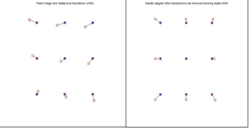
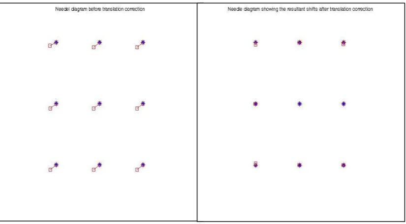
Figure 3.11: Translation and Radial Shifts ... 55

Figure 3.12: Estimated Radial Shifts after Translation correction ... 55

Figure 3.13: Near and far-focussed Images ... 56

Figure 3.14: Resultant shifts before translation correction (Left) and the Resultant shift after translation correction (Right) ... 57

Figure 3.15: Resultant shift before translation correction (Left) and Resultant shift after Translation correction (Right) ... 58

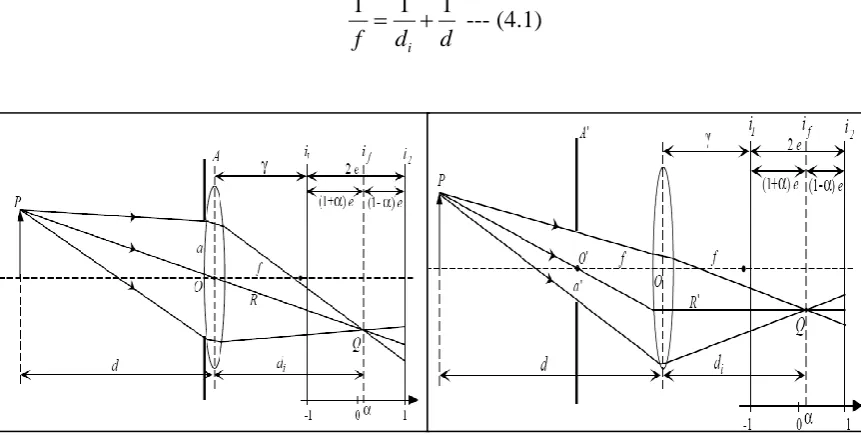
Figure 4.1a: Conventional DFD Optical Setup ... 62

Figure 4.1b: DFD system based on Telecentric optics ... 62

Figure 4.2: Defocus function (in-focus) - Spatial (Left) and 1D Frequency domain model (Right) ... 64

Figure 4.4: M

P

ratio vs. Normalised Depth ... 66

Figure 4.5: 2D discrete M P ratio space. ... 69

Figure 4.6: 1D plot of the designed rational filters ... 72

Figure 4.7: Model Verification Plot ... 75

Figure 4.8: Derived filter kernels for the defocus condition of 2.307 pixel ... 79

Figure 4.9: Magnitude responses of the designed filters for defocus condition of 2.307 pixels ... 80

Figure 4.10: Normalised depth vs. Theoretical M/P ratio for both the models ... 81

Figure 4.11: RMSE between Theoretical M/P ratio for both the models ... 81

Figure 4.12: Magnitude and Phase response of Gm1, Gp1, Gp2 and Pre-filter. ... 82

Figure 4.13a: Single frequency sinusoidal test pattern near-focused (Left) far-focused (Right) ... 83

Figure 4.13b: Depth map estimated using the filters designed by the proposed method (Left)and from Watanabe‟s filters (Right) ... 83

Figure 4.14: Single frequency sinusoidal test pattern with wavelength = 3.5 pixels ... 85

Figure 4.15: Depth Map for = 3.5 pixels (Left) and the depth map for = 3.2 pixels (Right) ... 85

Figure 4.16a: Actual vs. Estimated depth at different normalised depths using filters designed by Two Step Polynomial Approach and filters designed by Watanabe ... 86

Figure 4.16b: Standard Deviation plot at different depths for both the design models ... 86

Figure 4.17: Near and far focussed images ... 86

Figure 4.18: Gray scale depth map ... 86

Figure 4.19a: 3D view of the estimated depth ... 87

Figure 4.19b: 1D plot of the estimated depth using filters designed by both the models. .. 87

Figure 4.20a: Actual vs. estimated depth for filters designed by both the models ... 87

Figure 4.20b: Standard deviation plot at different depths for both the models. ... 87

Figure 4.21a: Actual Distance vs. Estimated Dist. (mm) ... 88

Figure 4.21b: Act. Dist. vs. RMSE (mm) ... 88

Figure 4.22a: Actual Distance vs. Estimated Distance (mm) ... 90

Figure 4.22b: Actual Distance vs. RMSE (mm) ... 90

Figure 4.23a: Actual vs. Estimated Distance (mm) ... 91

Figure 4.23b: Actual Distance vs. RMSE (mm) ... 91

Figure 4.24a: Actual Distance vs. Estimated Distance (mm) ... 93

Figure 4.24b: Actual Distance vs. RMSE (mm)... 93

Figure 4.25b: Working Distance for a 35mm lens with pixel size of 13µm against

different aperture settings ... 94

Figure 4.26a: Working Distance for a 50mm lens with pixel size of 7.4µm against different aperture settings ... 94

Figure 4.26b: Working Distance for a 35mm lens with pixel size of 7.4µm against different aperture settings ... 94

Figure 4.27: Magnitude plots of Gm1, Gp1, Gp2, and Pre-filter (left to right) designed for different experimental setups ... 96

Figure 5.1: Architecture of Virtex 2PX device ... 101

Figure 5.2: XUP 2VP Development Broad ... 102

Figure 5.3: Block Diagram - Internal architecture of XUP 2VP board ... 103

Figure 5.4: Example of 2D Convolution Operation ... 106

Figure 5.5: Diagram showing the independent coefficients of a 5x5 rotationally symmetric filter ... 108

Figure 5.6a: Frequency response Original and Conjugate... 109

Figure 5.6b: Rotationally Symmetric Low Pass filter ... 109

Figure 5.7a: 7x7 Image sub-block ... 110

Figure 5.7b: 7x7 rotationally symmetric filter with 8 fold symmetry... 110

Figure 5.8: Two Channel five stage pipelined architecture ... 112

Figure 5.9: Illustration of the Systolic movement of the data ... 112

Figure 5.10: Filter block module with Shift registers and FIFOs ... 114

Figure 5.11a: PSD of the checkerboard pattern for wavelength 8 ... 115

Figure 5.11b: Estimated depth map showing the artefacts ... 115

Figure 5.12a: PSD of checkerboard pattern for wavelength 10 ... 116

Figure 5.12b: Estimated depth map without the artefacts ... 116

Figure 5.13: Watanabe‟s pattern ... 116

Figure 5.14a: PSD of Watanabe‟s pattern ... 116

Figure 5.14b: Estimated depth map without post-processing ... 116

Figure 5.15: Comparison between Matlab frequency response and the scaled frequency response of the pre-filter ... 118

Figure 5.16: Generalised block diagram showing bit-widths at each stages of the pipelined processor ... 119

Figure 5.17: Near and far-focused images of the pattern ... 123

Figure 5.18a: Matlab 64 bit depth output with post-filtering ... 123

Figure 5.18b: Matlab truncated output with post- filtering ... 123

Figure 5.19a: FPGA depth map without post-filtering ... 124

Figure 5.19b: FPGA depth map with post-filtering ... 124

Figure 5.21a: Matlab 64 bit depth map with post-filtering ... 126

Figure 5.21b: Matlab truncated depth map with post-filtering ... 126

Figure 5.22a: FPGA depth map without post filtering ... 126

Figure 5.22b: Depth map with post filtering ... 126

Figure 5.23: Gray scale post-filtered depth map estimated from Matlab (left) and FPGA (right) ... 126

Figure 5.24: Matlab 64 bit post-filtered depth map ... 128

Figure 5.25: FPGA depth map without post-filtering (left) and with post-filtering (right) ... 128

Figure 6.1a: Sand paper pattern ... 132

Figure 6.1b: PSD plot of the sand paper pattern ... 132

Figure 6.2a: Actual vs. Estimated distance (mm) ... 133

Figure 6.2b: RMSE vs. Actual distance (mm) ... 133

Figure 6.3: 3D view of the scene and its corresponding real image ... 134

Figure 6.4: Near and far-focused images ... 134

Figure 6.5a: 64 bit Matlab post-processed output ... 135

Figure 6.5b: Matlab truncated post-processed output ... 135

Figure 6.5c: FPGA post-processed output ... 135

Figure 6.6: 3D view of the scene and its corresponding real image ... 136

Figure 6.7: Near and far-focused images ... 137

Figure 6.8a: 64 bit Matlab post-processed output ... 137

Figure 6.8b: Matlab truncated post-processed output ... 137

Figure 6.8c: FPGA post-processed output ... 137

Figure 6.9: 3D view of the scene and its corresponding real image ... 139

Figure 6.10: Near and far-focused images ... 139

Figure 6.11a: 64 bit Matlab post-processed output ... 139

Figure 6.11b: Matlab truncated post-processed output ... 140

Figure 6.11c: FPGA post-processed output ... 140

Figure 6.12: Wooden temple used in the experiment ... 141

Figure 6.13: Near and far-focused images ... 142

Figure 6.14a: Matlab depth map with 3x3 Gaussian smoothing ... 142

Figure 6.14b: FPGA depth map with 3x3 Gaussian smoothing ... 142

Figure 6.15: Sponge structure used in the experiment ... 143

Figure 6.16: Near and far-focused Images 3x3 Gaussian smoothing ... 143

Figure 6.17b: FPGA depth map with 3x3 Gaussian smoothing ... 143

List of Tables

Table 3.1: Shifts recorded on a conventional DFD lens systems ... 57

Table 3.2: Shifts recorded on a Telecentric DFD lens system ... 58

Table 4.1: Calculated values for the defocus function of 2.307 pixels ... 74

Table 4.2: Comparison of MSE between Linear Model and the Error Corrected Model ... 75

Table 4.3: Calculated values for the defocus condition 2.3587 e pixels Fe  ... 89

Table 4.4: Calculated values for the defocus condition e 2.3937pixels Fe  ... 92

Table 5.1: RMS error for different scaling factors ... 119

Table 5.2: Bit-width requirement for the four models considered along with the chip area used, and the RMSE between Matlab and FPGA depth outputs ... 120

Table 5.3: Delays at each stage of the pipelined architecture based on the simulation report ... 122

Table 5.4: Comparison between Matlab and FPGA depth outputs ... 124

Table 5.5: Comparison between Matlab and FPGA depth outputs ... 127

Table 5.6: Comparison between Matlab and FPGA depth outputs ... 128

Table 6.1: Comparison between Matlab and FPGA depth outputs ... 135

Table 6.2: Comparison between Matlab and FPGA depth outputs ... 138

Acknowledgements

For the past four years, I have been working on my Ph.D. research project concerning optical depth measurement. The thesis is the result of my study on this topic, which would not have happened without the help of many people. At this moment I would like to thank all those who have encouraged me towards the study. First and foremost, I would like to thank my supervisor: Dr. Richard Staunton for his continuous guidance and support over the last four years.

I would like to thank my colleague, Mr. Sheng Cheng for providing helpful advice on the use of FPGA‟s.

I am grateful to Mr. Charles Joyce for constructing the miniature models or real objects used in the experiments.

I would personally like to thank my brother, Mr. Anil Kumar and my brother-in-law, Mr. Saju Rebello for providing great emotional and financial support.

The University of Warwick has funded this research in the form of a Warwick Post Graduate Research Fellowship, I am really grateful to them.

Dedication

Declaration

This thesis is submitted in partial fulfilment for the degree of Doctor of Philosophy under the regulations set out by the Graduate School at the University of Warwick. This thesis is solely composed of research completed by Alex Noel Joseph Raj under the supervision of Dr. Richard Staunton.

Abstract

The science of measuring depth from images at video rate using „defocus‟ has been

investigated. The method required two differently focussed images acquired from a single view point using a single camera. The relative blur between the images was used to determine the in-focus axial points of each pixel and hence depth.

The depth estimation algorithm researched by Watanabe and Nayar was employed to recover the depth estimates, but the broadband filters, referred as the Rational filters were designed using a new procedure: the Two Step Polynomial Approach. The filters designed by the new model were largely insensitive to object texture and were shown to model the blur more precisely than the previous method. Experiments with real planar images demonstrated a maximum RMS depth error of 1.18% for the proposed filters, compared to 1.54% for the previous design.

The researched software program required five 2D convolutions to be processed in parallel and these convolutions were effectively implemented on a FPGA using a two channel, five stage pipelined architecture, however the precision of the filter coefficients and the variables had to be limited within the processor. The number of multipliers required for each convolution was reduced from 49 to 10 (79.5% reduction) using a Triangular design procedure. Experimental results suggested that the pipelined processor provided depth estimates comparable in accuracy to the full precision Matlab‟s output, and generated depth maps of size 400 x 400 pixels in

13.06msec, that is faster than the video rate.

Abbreviations

ASIC Application Specific Integrated Circuits

BRDF Bidirectional Reflectance Distribution Function

BSB Base System Builder

CC Correlation Coefficient

CCD Charge Couple Device

CLB Configurable Logic Blocks

CS Complex Spectrogram

DAQ Data Acquisition System

DCM Digital Clock Manager

DDR2 SDRAM Double-Data-Rate Synchronous dynamic random access memory

DFD Depth from Defocus

DFF Depth from Focus

EDK Embedded Development Kit

ESF Edge Spread Function

FFT Fast Fourier Transform

FIFO First In and First Output

FPGA Field Programmable Gate Array

IOB Input Output Block

LOG Laplacian of Gaussian

LSF Line Spread Function

LUT Look Up Tables

M P

Amplitude ratio between the differences of the amplitude of the defocused images to the sum

MAP Maximum a Posteriori

MHz Mega Hertz

MRF Markov Random Field

MSE Mean Square Error

PE Processing Elements

PLB Processor Local Bus

C

C

H

H

A

A

P

P

T

T

E

E

R

R

1

1

I

In the real world, objects are perceived in three dimensions (3D); length, breadth and depth. Humans observe 3D by utilising one or a combination of the available depth clues:- texture blur; edge blur, size perspective; binocular disparity; motion parallax; occlusion effects; and variations in shading [20]. The problem arises when the 3D objects are imaged by a photographic system. Here a 3D plane is mapped on to a 2D plane with reduced height and width information. The task of retrieving the depth information from one or more 2D images is an active research topic within the broad area of Computer Vision. The recovered depth information plays a vital role in Industrial and Medical applications such as component inspection, robotic manipulations, autonomous vehicle guidance, and 3D endoscopy.

The image formation process provides a geometric correspondence between the points in the 3D scene and the 2D image. In Perspective Projection, the light rays from the object that pass through a pinhole aperture define the image. Here each point in the image corresponds to a particular point of the object. In Orthographic Projection, light rays parallel to the optical axis form the image. By hypothesis, it corresponds to perspective projection when the camera is at an infinite distance from the object, and the lens has an infinite focal length. Figures (1.1a) and (1.1b) explain perspective and orthographic projections, where the x, y plane lies perpendicular to the optics axis and the z direction along it. It is the x, y image plane that provides the data for the range calculation.

Figure 1.1a: Perspective Projection [53] Figure 1.1b: Orthographic Projection [53]

Passive methods imitate the human biological vision system and therefore constantly search for „depth clues‟ within the acquired images. They are not limited to any

environmental constraint and find usage in military, medical and industrial applications [20]. The research here has concentrated on passive optical depth recovery. A brief description of passive depth recovery is presented in the next Section.

1.1. Passive Depth Recovery Methods

Optical depth estimation techniques can be categorized as Monocular or Binocular. Monocular techniques allow depth estimation using a single camera by considering depth clues such as the relative size of the objects, the distribution of light and shade, movement parallax of subject and background, and by measuring the amount of focus or defocus [20] [40] [93]. Binocular vision techniques require at least two images acquired from different viewpoints. These images are compared and the disparity between the images is related to the actual depth. Depths from Stereo and Structure from Motion are examples of Binocular vision techniques. Shape from Shading, Shape from Silhouettes, Depth from Focus and Depth from Defocus are instances of Monocular vision techniques.

P

Pinhole aperture

Image Plane Z

Y

X P

’

Object Plane

P ’

Image Plane Z

Y

X

1.1.1. Depth from Stereo

A simple stereoscopic system requires two images captured from different viewpoints. The viewpoints are separated by a suitable distance so as to provide two disparate images. The depth information is recovered by calculating the disparity information between these images. The typical stereo system is shown in Figure (1.2).

Figure 1.2: Depth from Stereo [20]

The two images, Im1 and Im2of the object P (see Figure (1.2)) are captured at two

different viewpoints separated by a baseline distance B. If f is the focal length of the lens and d is the stereo disparity between the objects in the images, then the depth of the object z is inversely proportional to the disparity and is given by [20]

d d B f

z (  ) --- (1.1)

The major difficulty in stereo imaging arises when establishing the correspondence between the objects in the two images. This process requires unique matching points to establish a pairing relationship and proves uncertain when the scene under investigation has:- (1) uniform intensity; or (2) is prone to occlusion effects (missing part problem) [20] [93]. Stereo pair analysis based on edge data has been presented by Baker [94], where the correspondence problem was solved by using an edge

X

X

P Image Im1

B

Lens Centre

Optical axis (x1,y1)

(x2,y2)

Y Image Im2

correlation procedure. Marr and Poggio [95] tackled the correspondence problem by considering a cooperative computational procedure. Their work was motivated by results of Julesz [96] on random-dot stereograms, which suggested that monocular vision does not provide any high level clue for disparity analysis [20], but in 1987 Pentland re-examined monocular technique and suggested that blurred edges can provide valid depth clues [1]. Marr et al. [97] [98] presented an algorithm that was analogous to the low-level human biological system. The disparity information was obtained from the zero crossing of the edges extracted from the right and left images, and the correspondence problem was solved by using disparity matches of gross line structures [93]. Stereopsis is analogous to the human visual system. It can provide dense depth maps, since an entire frame can be processed and depth estimates can be recovered for each pixel. Further, the depth maps generated are reliable, since there is no mechanical movement involved in the whole process.

1.1.2. Structure from Motion

required depth. Like stereo, SFM techniques also suffer from correspondence matching problems, and reliable depth maps are achieved only when accurate matching points are available. Further, these techniques require high resolution images to accurately determine the motion parameters. Additionally, SFM techniques are sensitive to the presence of noise in the observation and prove expensive in terms of storage and computation [20].

1.1.3. Shape from Shading

Shape from Shading (SFS) refers to the problem of extracting surface orientation from the gradual variation of brightness (shading) in the image [65]. Horn [53] discovered that the 3D shape of a surface can be recovered from a single image by considering the surface reflectance properties and the spatial distribution of the light sources. The brightness of the surface is described by the Bidirectional Reflectance Distribution Function (BRDF), which is the ratio of the radiance of the surface patch as viewed from the direction (θe,φe) to the irradiance resulting from illumination

from the direction (θi,φi) (see Figure (1.3)).

Figure 1.3: Structure from Shading [53]

The reflectance map, R(p,q), describes how the target radiance varies with the surface orientation for a given source distribution. It also presents a relationship for 3D shape recovery in terms of brightness (shading). This relation is expressed by Horn [53] in terms of image irradiance and is given by the equation,

Surface normal ň

(θi,φi)

R(p,q) = E(x,y) --- (1.2).

Here p,q denote the slopes of the surface along the x and y directions, and E(x,y) denotes the intensity at points x and y. The idea is to first compute the reflectance map, R(p,q) of the scene and then determine the gradients p,q for each point along x and y for a set of R(p,q) = E(x,y) equations with different light source positions. The camera and the scene are kept stationary [93]. SFS techniques are divided into four main approaches:- minimization, propagation, local and linear. A detailed report on the performance of these techniques is presented in [65]. SFS techniques require a prior knowledge of the scene reflectance and hence are not suitable for arbitrary scenes whose reflectance is unknown. Moreover, these methods cannot recover absolute depth and thus depend on a hybrid algorithm (mostly combined with stereo) to generate a reliable depth map [20] [65]. Further, the shape information from shadow areas is not recovered and so additional information has to be provided via techniques such as Shape from Shadow [65].

1.1.4. Shape from Silhouettes

to reconstruct these regions. An improved surface reconstruction algorithm that aggregated the local surfaces constructed by the 3D convex hull method has been presented by Shin and Tjahjadi [104]. They used the connectivity information of an octree and provided an improved surface reconstruction for the imperfect MC result. SFSh methods are particularly good when crude 3D models of the real world objects are required, and hence find usage in commercial 3D modelling packages [105]. However they suffer the drawback that the shape reconstruction could be affected by the type of the object and also by the camera position.

1.1.5. Depth from Focus

In Depth from Focus (DFF), the knowledge of the camera parameters is used to estimate the depth of an object. The sharpness of focus is measured on a sequence of images captured over a range of lens positions and related to the actual depth using the lens law [43]. A typical setup for estimating the range using focus is shown in Figure (1.4).

Figure 1.4: Depth from Focus

For an aberration free convex lens, when the object O at distance u from the lens is in focus, the image I is formed at a distance v on the image sensor. The relation between the focal length of the lens f, the object distance u and the image distance v is given by the lens law:

v u f

1 1 1



 ---- (1.3). f

u v

Object Plane

Image Plane

O Image

In DFF, the idea is to obtain a sharply focused image by adjusting either the focal length f or the image distance v or both. The measured f and v are substituted in equation (1.3) to determine the object distance u. In practice, a series of images are captured by continuously varying the image distance and the sharpest image for each object is found by employing a focus measure operator. Jarvis [73] suggested three focus measures based on computational simplicity, effectiveness, consistency, and implementation feasibility. They are: - (1) entropy; (2) variance; and (3) sum modulus difference. Darrell and Wohn [39] employed Laplacian and Gaussian pyramids to measure the sharpness criterion. A pipelined processor capable of generating a depth map in 10sec was also presented. The other researchers who actively contributed to DFF are Subbarao [92], Grossman [4] and Nayar [75]. Depth estimation using the focus criterion is a simple procedure that provides a direct relation to the actual depth using the lens law. It is monocular (only one camera position is involved) and hence does not suffer from the correspondence problem. Further, no additional hardware is required except for a computer controlled motor to adjust the lens position. DFF is essentially a search technique that requires the acquiring and processing of at least 10 to 12 images. This forms the fundamental weakness of the method since additional time is required to adjust the camera parameters before capturing each image. Further, during the entire period of adjusting the camera parameters the scene must remain stationary.

1.1.6. Depth from Defocus

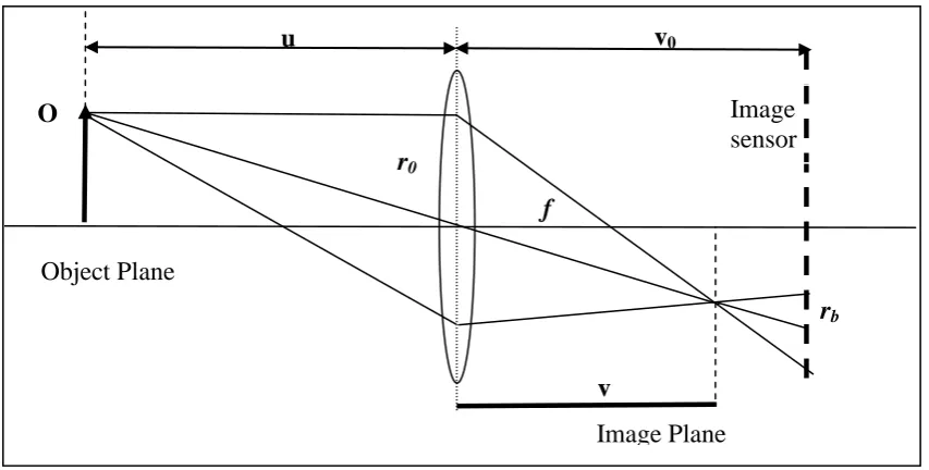
The Depth from Defocus (DFD) technique is based on the inherent inability of a practical optical system to focus at all distances in a scene. When a point light source is in focus, all the rays radiated from the object that are intercepted by the lens converge at a point on the image plane. But when the point light source is not in focus, its image is not a point but a blurred circular disc of finite radius rb. The disc

Figure 1.5: Depth from Defocus

In Figure (1.5), u refers to the object distance, v denotes the distance from the lens to the focused image, v0 refers to the distance between the lens and the image sensor, r0

refers to the radius of the lens aperture and rb denotes the blur circle radius. From the

lens geometry and the similarity of triangles, the blur circle radius is given as

) 1 ( 0 0   v v r

r_b ---- (1.4)

From the lens law,

u f v 1 1 1 

 . Substituting v 1

in equation (1.4) gives the relationship

between blur circle radius and the object distance as

) 1 1 1 ( 0 0 0 u v f v r

r_b    ---- (1.5)

The blur radius rb can be either positive or negative depending on whether the object

is in front or behind the focused plane. The ambiguity can be overcome by constraining the sensor distance v0 to be always greater than the image distance v. In

this case the depth is recovered only if prior knowledge of the scene‟s characteristics is known. To overcome this constraint, researchers have suggested the use of two images acquired on either side of the focused image. These images (near and far-focused) are identical except for the degree of blurring. The change in blur information is used to recover the depth information. Depth estimation is based on modelling the defocused image as the convolution between the focused image and the 2D Point Spread Function (psf) of the lens. Three different psf models have been

considered by researchers. They are: - (1) Gaussian; (2) Pillbox; and (3) Generalised Gaussian. A detailed review of the DFD techniques with their merits and demerits is presented in Chapter 2. Unlike DFF, the DFD methods do not search for the best focused image and hence require only a few images (usually 2) to provide a reliable depth map. Further, there is no correspondence matching problem as is attributed to the stereo and motion algorithms. DFD finds usage in applications where the imaging geometry prevents the use of multiple viewpoints. The limitations of DFD include [20]:- (1) Need for accurate modeling of the optical system; (2) Ensuring a sufficient amount of spectral information to measure the blurring between the images; (3) Edge bleeding due to windowing and (4) Need for accurate calibration of the camera parameters.

Passive depth recovery methods have their own limitations and can suffer from one or more of the following drawbacks:-

(1) Missing parts and the correspondence matching problem. Stereo and SFM techniques suffer from the above problem. Depth estimation is possible only at places where features are matchable, and thus require interpolation techniques to provide a dense depth map. Further, SFM techniques involve solving nonlinear equations by optimisation and thus require good initial guesses to arrive at a favourable solution.

(2) Controlled illumination requirement. SFS techniques do require environments which can offer control over the incident illumination. Since these techniques rely on accurate modelling of the surface reflectance, they are not suitable for complex natural scenes with arbitrary depths. Further, depth recovery is not possible for regions in shadow.

DFD techniques do have their own limitation (refer to Section 1.1.6) but due to their simplicity in operation, they can compare favourably to other depth estimation methods. With passive illumination, they require a minimum of two images acquired from the same viewpoint to produce a dense depth map, and thus can be useful for real-time depth recovery systems and for auto-focussing applications. Moreover, Schechner and Kiryati [88] claimed that for the same physical dimension, the DFF and DFD systems do not completely avoid the occlusion problem, but they are more stable in the presence of such disruptions than stereo. In addition, DFD methods are robust, since they involve modelling a single 2D psf rather than two distinct responses as in stereo. Considering the advantages of the DFD technique over other optical range methods, this research work investigates the use of the passive DFD method to develop a real-time depth / shape recovery system. The novelty lies in designing the texture invariant broadband filters using the Two Step Polynomial Approach and implementing the DFD algorithm on a Field Programmable Gate Array. A detailed report is presented in later chapters.

1.2. Organisation of the thesis

Chapter 2: Provides a detailed review of existing DFD techniques. The techniques were categorized based on: - (1) The method, active or passive; (2) The number of images required; and (3) The mode of operation. Further, the merits and the limitations of each technique along with the achieved depth accuracy are reported. A comparison Table based on the above categories is presented in Appendix 5.

Chapter 4: Presents a novel design procedure that determines the rational filter

coefficients by accurately modelling Watanabe and Nayar‟s M

P ratio curves [14]. The method referred as the Two Step Polynomial Approach determines the filter coefficients by considering the discrete

M

P ratio space. A comparison study is presented to determine how well the filters designed by both the Watanabe and the Two Step Polynomial

Approach fit the theoretical M

P ratio curves. Further, the depth estimation results for a single frequency test image and a real checkerboard image are presented. In addition, the chapter also investigates the effects of focal length, the aperture diameter, and the pixel size of the sensor on the rational filter‟s design, and on the working distance of a given experimental setup.

Chapter 5: Presents a hardware implementation of the DFD algorithm on the Virtex 2P FPGA. A pipelined architecture with two separate channels was employed to implement the five filtering stages in parallel. Further, a procedure referred as the Triangular method was used to reduce the number of multipliers required for the convolution process. Finally, a comparison study is performed where the depth results from the pipelined processor are compared against the full precision Matlab output.

Chapter 6: Presents depth estimation results for 3D objects with natural textures. Again, a detailed statistical comparison is presented for the depth estimates obtained from Matlab and from the pipelined processor.

C

C

H

H

A

A

P

P

T

T

E

E

R

R

2

2

R

R

e

e

v

v

i

i

e

e

w

w

o

o

f

f

t

t

h

h

e

e

D

D

e

e

p

p

t

t

h

h

f

f

r

r

o

o

m

m

D

D

e

e

f

f

o

o

c

c

u

u

s

s

T

T

e

e

c

c

h

h

n

n

i

i

q

q

u

u

e

e

s

s

Introduction

Depth from Defocus (DFD) methods like any ranging techniques can be broadly classified as Active or Passive. Active methods required an external illumination pattern to be projected under controlled environmental conditions on to the object that requires measurement, whereas Passive methods recover depth under ambient lightning conditions. However, if the scene under investigation has weak texture or is textures-less, then the only possibility is to employ an active illumination.

Early methods [1] [2] [5] were based on single images, where the defocus information was obtained from the blur measurement. These techniques required prior knowledge of the scene and were sufficient enough to recover depth only at certain image contours [15]. DFD methods for arbitrary objects using multiple images (two or more) have been proposed by many researchers. These methods can be further classified based on the mode of operation as Spatial, Frequency, Wavelet or Statistical techniques.

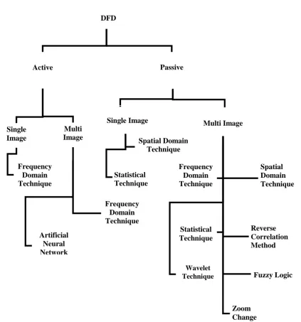
In this chapter an attempt has been made to categorize the available DFD techniques based on (1) The method, active or passive; (2) The number of images required, single or multiple images; and (3) The mode of operation, spatial domain, frequency domain, statistical, wavelets and other un-conventional techniques. Figure (2.1) illustrates pictorially the available DFD methods based on the above categories. The chapter first explains the Passive methods where an in-depth analysis of the DFD techniques is reported based on the proposed categories. Section 2.1.1 describes the single image passive DFD techniques and Section 2.1.2 describes the multiple image passive DFD techniques. Later, Section 2.2 describes the active methods which are classified as per the categories. A comparison chart is presented in Appendix 5, where the detailed information about the authors, their techniques, the merits and demerits of their method, and the achieved depth accuracy is reported.

Figure 2.1: Pictorial representation of the available DFD methods based on the categories.

DFD

Active Passive

Single Image _{Multi Image}

Frequency Domain Technique

Spatial Domain Technique

Statistical Technique

Zoom Change

Wavelet Technique

Statistical Technique

Spatial Domain Technique Multi

Image Single

Image

Frequency Domain Technique Artificial

Neural Network

Reverse Correlation Method

Fuzzy Logic Frequency

2.1. Passive Methods

Passive DFD methods are attractive since they estimate the depth of the scene under the ambient conditions. They avoid the usage of any illumination patterns and hence are suitable for depth as well as shape recovery. The main disadvantage which is common to any passive technique is the requirement of a textured pattern since a texture-less object will „look the same‟ whether focused or unfocussed. This Section describes the available passive DFD techniques.

2.1.1. Single Image Techniques

Alex Pentland was the first investigator who employed „defocus‟ as a clue to estimate the depth of an object. He observed that Depth from Focus (DFF) techniques and auto-focussing algorithms employed an exhaustive search mechanism to find the „best‟ focussed image from a collection of 30 or more images. These

techniques were time consuming and required sophisticated parallel hardware for effective operation. He realised that search for the best focused image was unnecessary and presented a novel method where the depth was estimated from a single image by measuring the error in focus; the focal gradient [1]. The amount of defocus (blurring) was related to the distance of the object from the focused image and the characteristics of the lens. The object depth D was measured using the relation,

F f v

fv D



  

0 0

---- (2.1)

where, f was the focal length of the lens, v0 the distance between the lens and the

image plane, F the f-number of the lens1 and  the spatial constant of the 2D Gaussian psf of the defocused lens. The only unknown in equation (2.1) is  of psf which is a measure of the rate of change of image intensity at sharp discontinuities in the images (e.g. edges). A Laplacian operator was employed and the zero crossing of the Laplacian provided the maximum rate of change of image intensity i.e. the edges. By using a linear regression model,  was estimated and substituted in equation (2.1) to obtain the object distance. Although the method looked simple it had two main disadvantages :- (1) The method required the prior knowledge of the scene

characteristics and hence could be used to measure depth only at step discontinuities; and (2) the ambiguity whether the image was formed in front or behind the plane of exact focus had to be overcome by a suitable scene setup. These demerits were later addressed by Pentland [1] [2] by considering two images of the same scene taken with different aperture settings. The algorithm had the potential to produce depth plane segmentation but was not accurate enough to produce a dense depth map. Grossman [4] has achieved an accuracy of1.25cm using the above method.

After Pentland, Subbarao and his research associates were the most active advocates of the DFD method. In 1988, Subbarao and Gurumoorthy [5] proposed a method similar to Pentland‟s [1] where the Line Spread function (LSF) corresponding to the

psf of the lens was computed from a blurred edge. The spread of the LSF, measured from the second central moment (standard deviation distribution of the LSF) was linearly related to the inverse distance using the equation

c mu

l  

1

 --- (2.2)

where, _l was the spread of the LSF, m and c were the camera parameters and u-1 the object distance. The approach differed from Pentland‟s in the computational simplicity of measuring the magnitude of the blurred edge and relaxed the assumption that the psf to be modelled was Gaussian. Here the psf was considered to be rotationally symmetric. The algorithm works well on isolated edges but causes depth estimation errors in the presence of other edges.

Lin and Gu [69] proposed a model that estimated the blur by employing a histogram technique that measured the pixel intensity distribution of a single image. The estimated histogram was then related to the actual depth using a pre-calibrated mathematical model. Experimental results with real images suggested a RMS error less than 3% when the furthest point was at 1200mm.

Namboodiri and Chaudhuri [67] proposed a statistical method based on the inhomogeneous reverse heat equation that estimated the blur information and depth perception using a single image. The model formulated the Gaussian psf in terms of the heat equation and related the blurring parameter to the diffusion coefficient as

 2 tc

of the blur in terms of pixel units. The heat equation was inhomogeneous since the coefficient c and the time t are related to the depth location. The depth information was measured as a disparity between the observed image and the reconstructed image, and the estimated depth map was further refined using a Markov Random Field (MRF). Although the depth map was retrieved from a single image, it was actually similar to Favaro‟s multi-image diffusion method [68]. Theoretical results were not provided due to the ambiguity of whether the object was in front or behind the focussed image.

2.1.2. Multiple Image Techniques

With multiple image techniques, two or more images acquired with different camera settings are compared to provide the required depth estimate. The methods offer two main advantages over the single image technique: - (1) They avoid the extensive pre-calibrated depth model required for single image techniques [69], since the ambiguity whether the object is in front or behind the focus plane has been overcome; (2) They do not require any prior knowledge of the scene and hence can be applied for arbitrary objects with any random shape. Further, the Section provides a sub-classification based on the core technique used.

2.1.2.1. Frequency Domain Techniques

Pentland‟s second approach [1] [2] was based on a multiple image frequency domain

Figure 2.2: Passive DFD optical setup based on Pentland‟s approach [1]

In practice the images were first convolved with a 8x8 Laplacian filter and averaged using a 8x8 Gaussian filter to produce a „power image‟. This provided an estimate of the power of the central spatial frequency of the Laplacian filter at each image location. The two transformed images were then compared and a look up-table was used to estimate the depth. The algorithm was implemented on a Datacube image processing system and included a beam splitter to capture two images simultaneously as shown in Figure (2.2). The system processed 8 frames per second with an accuracy of 6% standard error over a 1 cubic meter measurement volume. The accuracy was improved to 2.5% standard error by considering a Laplacian pyramidal architecture where the Fourier powers were estimated at several frequencies instead of single frequency. The disadvantage of the algorithm was its assumption that one of the images was taken using a pin-hole camera which was unacceptable as such a tiny aperture required a long exposure time and produced diffraction effects that were more pronounced as the width of the aperture was decreased [53].

Subbarao [6] relaxed Pentland‟s requirement of a pinhole aperture and recovered

depth by considering two images (which may or may not be in focus) acquired with different camera settings. The depth was recovered by changing: - (1) The distance between the lens and the image detector; (2) The focal length of the lens; and (3) The aperture diameter. The ratio of the Power Spectral Density (PSD) over a small local

Viewed 3D object

Beam Splitter

Large Aperture Camera

area was employed to estimate the spread parameter ( 1, 2) of the two defocused

images. These were then related to the inverse of the actual depth by equation (2.2). Experiments proved that the computed  was strictly a monotonic function between two set intervals and provided accurate depth results for nearby objects. For far away objects the method provided qualitative information.

In [7] [10], Subarao and Wei employed the DFD technique for autofocus applications. The method referred to as DFD1F, was based on computing the one dimensional Fourier coefficients as opposed to two dimensional and hence provided computational advantage and robustness for practical applications. The approach was based on the accurate calibration of the psf which was computed from the LSF of blurred step edges as explained in [5]. In actual practice, the estimated blur parameter

 was used as an index for a look-up table that provided a calibrated psf, modelled either as a Gaussian or a Pillbox. It was reported, that for low levels of blur the Gaussian psf model provided better results than the Pillbox, and for higher blur levels the Pillbox proved more accurate. The algorithm was implemented on their SPARCS camera system, and provided an accuracy of 3.7% RMS error for auto-focusing applications over a distance of 0.6m to infinity. For ranging application, the RMS error was 4% at 0.6m and linearly increased to 30% at 5m distance.

In 1995, Xing and Shafer [50] [54] used a large bank of Moment filters to estimate the depth information of the scene. Moment and Hyper-geometric filters were narrow band and hence estimated the spectral power at a large number of individual frequencies. The recursive properties of the filters allowed the effects of finite width windows and fore-shortening (caused by non-stationary transformation between two images) to be explicitly analysed and eliminated [54]. Two variants of their algorithm were proposed: - (1) Moment filters without slope estimation (MFF1); and (2) Moment filters with slope estimation (MFF2). Both the techniques were compared with Subbarao‟s frequency domain method [6]. It was reported that the RMS error of the estimated depth map using Subbarao‟s method was 4 times higher

In 1998, Watanabe and Nayar [14] provided an improvement to the existing methods

[1] [2] [6] [50] by considering the normalised M

P ratio of the defocused images (amplitude ratio between the difference of the amplitude of the defocused images to the sum) instead of the conventional amplitude ratio. A set of broadband filters were

designed in the frequency domain that accurately modelled the M

P ratio curves. Since the filters were broadband in the frequency domain they were narrow-band in the spatial domain and hence suitable for real-time implementation. A Pillbox psf model was considered for the implementation and four 7x7 2D texture invariant filters (including a pre-filter) were designed to effectively retrieve the depth information. It was reported that the depth detection error was less than 1% irrespective of the texture frequency. The depth accuracy was between 0.5% and 1.2% with respect to the distance from the lens. Though real-time implementation was not presented, the authors have claimed that by using their customised Datacube MV200 pipeline processor, the algorithm can deliver six depth maps of size 512 x 480 pixels in one second.

The magnification variation between the defocused images was addressed by Watanabe and Nayar [41] by employing telecentric optics. An aperture stop was introduced at the front focal plane of the lens and a FFT phase based local shift detection method was employed to detect the magnification changes. The magnification was reduced to 0.03% from 3% (reported by Subbarao in [8]) by employing the telecentric aperture.

Raj and Staunton [87] proposed a technique based on Phase Correlation [28] [29] [30] to determine the magnification change between the defocused images. The method considered the magnification change within the sub-block as a local translation problem and estimated the shift by inverse transforming the normalised Cross Power Spectrum. The approach was more practical and robust to noise than Watanabe‟s method which determined the shift by fitting a plane to the noisy phase

Recently, Favaro and Duci [64] proposed two methods that exploited the results of Fourier analysis and Singular Value Decomposition (SVD) in the frequency domain to estimate the depth and the radiance of the scene. In their first method they considered the psf as a 3D Gaussian function and represented the imaging model as a convolution between the 3D psf and the transformed volume density (depth estimate). The method required a dense set of defocused images, usually more than 100 and employed deconvolution techniques [47] to estimate the depth. The maximum achievable accuracy for the given setup conditions can be determined directly from the model which was based on the camera settings, the number of input images and the resolution of the image. The second method considered the linearity of the imaging model and employed the SVD in the frequency domain to estimate the depth based on a least squares solution. The method required less than 5 defocused images and was stated to be efficient for practical purposes. For both the methods the radiance of the scene was reconstructed from the additional information provided from the geometry and photometry of the imaged scene. Though theoretical results were not provided, the authors have compared the results with their existing algorithm based on the least squares solution described in [66]. The depth maps and the radiance of the scene were recovered reasonably accurately.

2.1.2.2. Spatial Domain Techniques

In 1993, Ens and Lawrence [12] proposed a Spatial domain technique based on a matrix regularization approach to recover depth information from two defocused images. Their method was stated as an alternative approach to that of the inverse filtering methods advocated by Pentland in [1] [2], where windowing effects are more pronounced. They approached the problem by identifying the psf, h3(x,y) such

that

) , ( ) , ( ) ,

( 3 2

1 x y h x y h x y

h   --- (2.3)

where h1(x, y) and h2(x, y) are the psfs of the two defocused images and h3(x,y) is

the convolution ratio of the defocused operators h1(x,y) and h2(x,y) or the extra

defocus that is required to make h1(x,y) equal to h2(x,y). The estimated h3(x,y)

the best pattern of h3(x,y) from a pre-computed lookup table that minimized the objective function min )] , ( ) , ( ) , ( [ 0 0 2 2 3

1   



i --- (2.4).

Here i1(x,y) and i2(x,y) are the two defocused images. The lookup table was derived

based on the theoretical or experiment models of the psf. Results with theoretical psf models resulted in an RMS error of 1.7% in terms of distance but reduced to 1.3% when an experimental psf was used. The disadvantages of the method are that it was based on a smoothness assumption and it was computationally intensive [8].

An improved psf measurement technique was proposed by Claxton and Staunton [49]. The method employed a knife edge technique, where a super resolution Edge Spread Function (ESF), obtained by imaging a knife edge on a light box was differentiated to provide a more accurate model of the psf. The method proved simple and effective for shift invariant DFD models since the psf was averaged over the entire length of the edge. Three different psf models (Pillbox, Gaussian and Generalised Gaussian) were considered, and it was observed that the Generalised Gaussian model performed better over a wide working range with different aperture settings. The mean square error (MSE) of the fit of the psf using the Generalised Gaussian model was 8 times better than the Gaussian model and 14 times better than the Pillbox model.

Subbarao and Surya [8] actively employed their Spatial Domain Convolution/ Deconvolution Transform (S Transform) to effectively recover the depth information of an object in the spatial domain. Their method referred as „S‟ transform method

(STM) required only two or three blurred images and provided results that were comparable to Depth from Focus techniques. The forward „S‟ transform expressed the defocused image as a two variable cubic function using Taylor‟s series (equation (2.5)), and the inverse „S‟ transform (deconvolution operation) which provided the focussed image was obtained by subtracting a constant times the Laplacian of the blurred image from the blurred image, as given in equation (2.6)

mn _mn

n m n m h y x f n m y x

g , _,

3

0 _{! !} ( , )

) 1 ( ) , (



( , ) 4 1 ) , ( ) ,

(x y g x y 2 2g x y

f     --- (2.6).

Here, g(x,y) is the defocused image, f(x,y) the focused image, hm,n is the rotationally

symmetric psf,  the second central moment of the point spread function and 2 is the Laplacian operator. In practice the images captured using different camera settings (as explained in [6]) were approximated as focussed images within a small neighbourhood of 9x9 pixels and expressed as

( , ) 4 1 ) , ( ) ,

( _{1 1}2 2 ₁

1 x y g x y g x y

f     --- (2.7), and

( , ) 4 1 ) , ( ) ,

( _{2 2}2 2 ₂

2 x y g x y g x y

f     --- (2.8).

The depth was obtained by comparing the approximated focussed images as given by

2 2 2 2 1

2 1 2 1

( , ) ( , ) 1

( , ) ( , ) ( ) ( )

4 2

f x y f x y

f x y  f x y      --- (2.9).

where 12 and 2 2

 refer to the second central moment of the psf, and f1(x,y) and

f2(x,y) refer to the approximated focused images. The initial assumption that the

focused image should be modelled as a cubic polynomial was relaxed by using a generalized „S‟ transform which incorporated the use of smoothing filters proposed

by Meer and Wiles [11]. The estimated  was then linearly related to the inverse distance as given by the equation (2.2). Two versions of STM were implemented. In STM1, the diameter of the aperture was fixed and two images were taken by changing the lens position. The percentage error in terms of distance was about 2.3% at 0.6m and it linearly increased to about 20% at a 5m distance. In the STM2 the lens position was fixed but the diameter was changed and the RMS error estimated was similar to that of STM1. In the case of 3D objects the error depended on the shape and appearance of the objects. For objects with small depth variations STM calculates the average distance of the objects in the scene. Results on auto-focusing experiments suggested that STM performed better and faster for medium levels of blur, and the DFDIF [7] method proved more effective for higher levels of blur [10].

expressed as a function of the partial derivatives of the other image. Their 2D model involved the calculation of blur difference  which was obtained by solving four mathematical equations and determining the „best‟ through error analysis. The estimated  was then related to the inverse object distance as given in equation (2.10).         _    

 2 2

2 2 ) 2 ( 1 1 2 1 1 1 _    F v k

v v f v v F

z --- (2.10)

where z is the object distance,  is the blur difference between the defocused images and v, F, f , k are the camera parameters. Tests were performed on step edges, line edges and on junction like L, V, T, Y and X, and compared with Subbarao „S‟ Transform method [8]. It was observed that the latter method was capable of estimating the blur only at line edges. At step edges and on junctions the „S‟

Transform failed since Laplacian of Gaussian was zero at these points [23]. The RMS error reported for a planar object whose furthest point was at 125cm and the nearest at 115cm was 2.21% against 4.22% for Subbarao‟s „S‟ Transform method. The depth densities for the methods are 97.4% and 85.3% respectively. Considering the spatial errors involved in camera movements while image acquisition, Deschenes et al. [22] extended their Hermite Polynomial model to include the spatial shifts; horizontal, vertical, zooming and 2D motion. The RMS error reported was 1.68% with a depth density of 100%. An improvement of the above method was proposed in [61] where the spatial shifts and the zoom disparities were simultaneously computed along with the blur using a Homotopy based approach with several higher order derivatives calculated for the image.

spread parameter; however this introduced additional complexity in the image acquisition and increased the processing time of the algorithm.

Leroy et al. [60] extended the work of Simon et al. [58] [59] and proposed a simpler algorithm which required only two defocused images. Their work was based on Subbarao [8] and Deschenes [15] [21] [22], where the magnitude of the Laplacian gradient at the edges for step, ramp or roof was computed to determine the depth. Though real-time implementation was not presented, the authors have stated the algorithm could compute a depth map of 800 x 600 pixels in 23ms. The maximum mean depth error reported was 20.05mm between a range of 790mm and 990mm. The main drawback of the method was the influence of the edge density and the characteristic of the image textures on the accuracy of the estimated depth. It was stated in [60] that the edges with high density provided more accurate depth results.

In 2007, a neural network based technique was suggested by Jong [81] which estimated the spread parameter  of the Gaussian psf in the spatial domain. The model was based on a supervised learning network that employed the Radial Basis Function (RBF). The RBF was preferred over a Back Propagation network (BPN), since it provided a better approximation to a continuous function [82]. Experiments were performed on edges with objects placed between 220mm and 355mm. A 5% error relative to the object distance was reported.

The above mentioned techniques (except Favaro‟s and Chaudhuari‟s) considered the imaging model as a linear shift invariant system and expressed the defocused image as a convolution between the focused image and the shift invariant psf [53]. However, Tu et al. [83] proposed a technique based on inverting the shift variant blur model in the spatial domain to recover the depth and the focussed image from two defocused images. The method was an extension of Subbarao‟s „S‟ Transform approach [8] for shift invariant blur models, and incorporated Subbarao‟s Rao