Optimization in Diamond

(1)

1

Faculty of Behavioural,

Management & Social Sciences

Optimization in Diamond

Joris van der Meulen M.Sc. Thesis September 2016

(2)

(3)

Management Summary

Diamond is a decision making tool that enables users to construct models of

the processes that take place in dairy factories and optimize these processes by varying the product mix and technology settings in these models. Differential Evolution (DE), a stochastic optimization method, is implemented in Diamond

to perform these optimizations. DE’s effectiveness and efficiency depend on the values of several auxiliary optimization parameters. In the current situation, a

user of Diamond has to set values for those parameters before performing an optimization. The goal of this research is to find an approach for determining the values of DE’s auxiliary optimization parameters in Diamond so that they do

not have to be set by the user anymore.

We apply the approaches of parameter selection and meta-optimization to

tune the auxiliary optimization parameters of DE in Diamond. Parameter se-lection comes down to selecting values for the auxiliary optimization parameters relying on conventions and default values. Meta-optimization involves treating

the search for good auxiliary parameter values as an optimization problem in its own right. It hence requires the implementation of an optimization method on the

meta-level. The meta-level optimizer aims to find good values for the auxiliary parameters of DE, which in turn aims to find good values for the optimization variables of the actual problem in Diamond. We depict this process graphically

in Figure 1. We select the Nelder-Mead (NM) method as meta-level optimizer.

We evaluate three different performance aspects for our solution approach:

reliability, robustness, and efficiency. An assumption regarding meta-level search spaces based on which we selected the NM method as meta-optimizer does not

seem to hold, impeding on the reliability of our solution approach. We applied our solution approach 5 times to 3 different problems and it only yielded consistently good results for one of the problems, and failed to yield good results twice for both

other problems. Our solution approach appears to be quite robust against changes in the actual problem, but more tests in this direction have to be performed. Our solution approach seems efficient when we compare it to the strategy of selecting

commonly advised auxiliary optimization parameters from literature. However, it barely performs better (on the problem for which our solution approach yielded

consistently good results) than two straightforward strategies that use a similar

(4)

Problem in Diamond Differential Evolution

Figure 1: Meta-optimization in Diamond

amount of computation time and that do not rely on any assumptions regarding

meta-level search spaces for their reliability.

By applying parameter selection and meta-optimization, we have constructed

an approach for determining the values of DE’s auxiliary optimization variables so that they do not have to be set by the user anymore before performing an optimization, which was the goal of our research. We however conclude that our

solution approach, even though it is successful in tackling the research problem, is not very promising for Diamond. In particular, the NM method is not such a good

meta-optimizer. In a more general sense, the practical suitability to Diamond of the combined parameter selection and meta-optimization approach can be questioned. The biggest downside of this approach is that auxiliary parameters

resulting from a meta-optimization run cannot easily be generalized to different values for the auxiliary parameters to which parameter selection has been applied. We recommend further research aimed at improving the speed and quality of

our solution approach, such as making use of information that has been obtained in previous meta-optimization runs and parallelizing our solution approach. Our

main recommendations are on the deeper levels of Figure 1 though. We recom-mend further research in the field of (self-)adpative DE, in which feedback from the search progress is used to control the values of the auxiliary optimization

parameters. Adaptive DE variants usually introduce new auxiliary parameters whose values the user must decide upon, but these new auxiliary parameters are

generally a lot more robust than those of standard DE. It might therefore be pos-sible to determine values for the new auxiliary parameters that can be applied to Diamond in general instead of being suitable for only one problem and perhaps

other instances of that problem. Finally, information extracted from the actual problems and similarities between future problems in Diamond can potentially be used to develop an algorithm tailored specifically for Diamond that is more

(5)

Acknowledgements

I would like to express my gratitude to those who have helped me with my grad-uation assignment. First of all, I would like to thank Martijn and Marco, my

supervisors at the University of Twente, for their guidance and their critique. I would like to thank everybody at Reden and the team at FrieslandCampina, for making me feel welcome and taking the time to discuss my ideas about the project.

Special thanks go to Niels, who supervised me at Reden and frequently took the time to explain me something or help me out somewhere. Finally, I would like to

thank Sarah, my friends, and my family, for both the support and the distraction they have provided me with over the course of this assignment.

(6)

(7)

List of Abbreviations

DE Differential Evolution

DOE design of experiments

EA evolutionary algorithm

FC FrieslandCampina

GA genetic algorithm

HJ Hooke-Jeeves

LJ Luus-Jaakola

LUS Local Unimodal Sampling

NFL no free lunch

NLP nonlinear programming problem

NM Nelder-Mead

(10)

(11)

Chapter 1 Introduction

The research in this thesis revolves around Diamond, a project conducted by Reden and the FrieslandCampina (FC) department milk valorization. In this

project, a software solution is developed that is also called Diamond. Diamond is a decision making tool that enables users to construct models of the processes taking place in dairy factories and optimize these processes by varying the product

mix or technology settings in these models.

This chapter functions as an introductory chapter to Diamond and the

re-search we conduct. In Section 1.1 we briefly explain how Diamond works. We identify the research problem in Section 1.2 and determine the research goal in

Section 1.3. In Section 1.4 we introduce the research questions and describe the set-up of the remainder of this report based on those questions.

1.1 Diamond

Diamond is developed as a tool that can give decision-making support for two types of problems that FC frequently encounters in processes in their factories.

The first type of problem is related to raw material sourcing. Such problems arise when several raw materials or waste flows from other factories can be used for a certain process. The decision that has to be made in this type of problem is

which raw materials to use in the process and in what volume.

The second type of problem arises when a process consists of multiple steps

leading to several end products. In such processes there are variable technology settings that influence the product specifications of the end products and the amounts of products that are produced. The decision that has to be made in this

type of problem is what values to select for those technology settings.

In order for Diamond to give decision-making support for these problems, the

user has to provide the software with a problem that resembles the process in which the user wants this support. A problem in Diamond is defined by three

parts: a datastore, a network, and optimization variables. In this section we

(12)

briefly discuss each of these parts.

The network

A user of Diamond has to load or construct a network in Diamond. A network in Diamond is constructed by dragging elements onto a grid and linking them with

connectors. Those elements represent the inputs, outputs, and all intermediate steps of the process that is being modelled. In this report the inputs are referred to

as raws, the outputs as sales, and the intermediate steps as unit operations. The connectors represent the incoming and outgoing product flows of each element. Raws only have outgoing product flows, sales only have incoming product flows,

and unit operations always have both.

We present a screen capture of the interface of Diamond in Figure 1.1. This

screen capture is blurred for confidentiality reasons. It displays a network that we have constructed on the grid with elements and connectors. We have assigned a different colour to each element type. Raws are distinguished by their blue colour,

sales by their pink colour, and unit operations by their green colour. A list can be distinguished to the left of the grid in which the network is constructed. This list contains the elements that can be used in the network. It is provided by loading

a separate datastore in Diamond that defines these elements.

(13)

1.1. Diamond 3

The datastore

A datastore has to be loaded in Diamond to define the elements that can be

used for the construction of a network. When a user wants to load an already constructed network in Diamond, the matching datastore in which the elements that have been used for the construction of that network are defined has to be

loaded as well. In such a datastore the different elements are defined in the following way.

A raw is defined by a parameter vector in which the product specifications of

the raw are stored. With product specifications we mean the amount of each in-gredient in the product, the amount of each nutrient in the product, and product properties of interest, such as the viscosity and the water activity of the

prod-uct. A sale is defined by two parameter vectors that denote lower and upper bounds for its product specifications. A unit operation is defined by its ingoing

and outgoing product flows and the transfer functions between them. Since unit operations need to model every processing step that might happen in a dairy factory, there can be a large amount of transfer functions defining one unit

oper-ation and these functions can be complex. Transfer functions in a unit operoper-ation can depend on variables. We refer to those variables as the technology settings of that unit operation. A user can assign values to the technology settings of a

unit operation if that unit operation is used in the network.

The optimization variables

When a datastore and a network have been loaded or constructed in Diamond, optimization variables need to be selected. The technology settings of a unit operation can be optimization variables. The input volume of a raw can also be

an optimization variable.

Performing an optimization

When a network has been constructed and optimization variables have been se-lected, a user can click the optimize button in the lower left part of the interface. When this button is clicked, a dialog pops up in which the user can inspect the

technology settings and input volumes that are optimization variables. The user has to set values for several auxiliary optimization parameters in this dialog and can then start an optimization run. An optimization run takes minutes to hours,

depending on the size and complexity of the problem at hand. The values se-lected for the auxiliary optimization parameters also influence the runtime. Upon

(14)

op-timization variables that have been encountered during the run, the impact that those values have on the process, and the resulting profit. It is now up to the

user to adjust the product mix or technology settings in practice so that they match the values of Diamond, or decide not to.

1.2 Problem Identification

A user of Diamond has to provide the software with a datastore and a network of a process in which optimization variables are selected. In turn, after some

computation time, Diamond provides the user with hopefully near-optimal values for the optimization variables. In the context of Diamond, optimal values for the

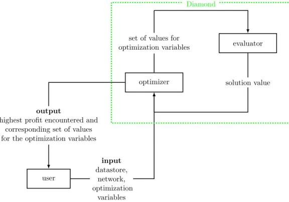
optimization variables mean those values that lead to the highest profit that can be obtained in the process that has been modelled. We depict this procedure in Figure 1.2. A part of this figure is enclosed by a green dotted line. This part

represents the software solution Diamond. An iterative procedure takes place within it.

evaluator set of values for

optimization variables

optimizer solution value

user

output

highest profit encountered and corresponding set of values for the optimization variables

input

datastore, network, optimization

variables

Diamond

Figure 1.2: How Diamond operates – a rough depiction

Diamond roughly consists of two parts. In one part, which we call the

(15)

1.2. Problem Identification 5

is evaluated. This solution value is related to the profit in such a way that a lower solution value generally corresponds to a higher profit. The other part

of Diamond is responsible for determining the sets of values for the optimiza-tion variables that have to be evaluated by the evaluator. We call this part the optimizer because it aims to find optimal values for the optimization variables.

To this end some of the evaluated solution values and their corresponding sets of values for the optimization variables are temporarily stored in the optimizer.

The best solution value that has been encountered is always stored and so is the corresponding set of values for the optimization variables.

The choice has been made by the developers of Diamond to treat the

evalu-ator as a black box, meaning that we can obtain an output from the evaluevalu-ator for a given input but have no knowledge of its internal workings. In the case

of the evaluator, the input is a set of values for the optimization variables and the output is the corresponding solution value, as can be seen in Figure 1.2. As soon as a datastore, a network, and optimization variables are defined, a

prob-lem in Diamond can be formulated as a nonlinear programming probprob-lem (NLP), because of which the evaluator’s internal workings are known. Although there are solution methods for solving specific types of NLPs by making use of certain

characteristics of their solution spaces, the NLPs resulting from the problems in Diamond have complex, multimodal1, non-continuous, non-linear objective

func-tions. Next to soft constraints that lead to a penalty in the objective function if, and based on the extent that, they are not satisfied, the NLPs resulting from the problems in Diamond also have hard constraints. Constrained NLPs with

com-plex, multimodal, non-continuous, non-linear objective functions are generally treated as black boxes because it is difficult to make useful assumptions

regard-ing their solution spaces. Furthermore, users of Diamond have a lot of freedom in determining the datastore, network, and optimization variables, because of which the internal workings of the evaluator vary. These are the reasons for treating

the evaluator as a black box.

Treating the evaluator as a black box, and hence ignoring any assumptions

that could possibly be made about the solution spaces of the problems in Dia-mond, brings along a problem. If no assumptions are made regarding a solution space, the no free lunch (NFL) theorem for optimization states that each

opti-mization method is as likely to find a good solution value as any other. Wolpert and Macready (1997) prove this by showing that, for an arbitrary measure of performance, the probability of obtaining a specific sequence of solution values,

1

(16)

averaged over all possible functions, is independent from the applied algorithm. In other words, one could not expect to find an optimization method that

per-forms any better than any other optimization method (Jansen, 2013).

There are solution methods that, by incorporating auxiliary optimization

pa-rameters, can overcome the implications of the NFL theorem. These solution methods are called metaheuristics and they can be efficient on a wide range of problems provided that they are well parametrized (Luke, 2013). One of those

metaheuristics has been implemented in the optimizer in Diamond.

Differential Evolution (DE) is the metaheuristic that has been implemented in

the optimizer in Diamond. We explain how this metaheuristic works in Chapter 2. DE has been selected by the developers of Diamond because it is a competitive metaheuristic with relatively few auxiliary optimization parameters. It has been

shown that DE is efficient in a wide variety of practical as well as theoretical problems (Das & Suganthan, 2011; Civicioglu & Besdok, 2013; Lampinen, Storn,

& Price, 2005, pp. 156-182). Like any metaheuristic though, values have to be selected for several auxiliary optimization parameters in order for DE to perform well. At the moment it is the case that a user of Diamond has to choose values for

those parameters before performing an optimization. FC however does not want Diamond to require any optimization-related input from its users other than the

datastore, the network, and the optimization variables. This brings us to our problem statement: Values for the auxiliary optimization parameters of DE have to be set by the user before performing an optimization in Diamond.

1.3 Research Goal

We formulate our research goal based on the problem statement that we have defined in Section 1.2. We formulate the research goal as follows: Find a way to determine values for DE’s auxiliary optimization parameters so that they do not

have to be set by the user before performing an optimization in Diamond.

1.4 Research Questions

To conduct research in a structured manner, we formulate several research ques-tions. Based on the problem statement that we have formulated in Section 1.2

and the research goal that we have defined in Section 1.3, we formulate the fol-lowing main research question: How can we determine values for DE’s auxiliary

(17)

1.4. Research Questions 7

that support the main research question:

RQ 1. What is the current situation?

1(a). What problems for Diamond do we have at our disposal?

1(b). How does DE work and what are its auxiliary optimization parame-ters?

RQ 2. What approaches for determining values for auxiliary optimization pa-rameters can we find in academic literature?

RQ 3. What is a good approach for determining values for DE’s auxiliary opti-mization parameters in Diamond?

RQ 4. How does the proposed approach perform?

In Chapter 2 we discuss research question 1. We introduce three problems

from practice and explain the workings of DE in this chapter. In a literature review in Chapter 3, we discuss research question 2. In Chapter 4 we answer

research question 3 by proposing an approach for determining the values of DE’s auxiliary optimization parameters in Diamond. We discuss the performance of this approach in Chapter 5 and answer research question 4 this way. In Chapter

(18)

(19)

Chapter 2 Current Situation

In this chapter we give an overview of the current situation. We introduce the

three problems from practice that we have at our availability in Section 2.1. In Section 2.2 we describe how DE, the metaheuristic that is implemented in

Diamond, works and identify the auxiliary parameters that a user of Diamond currently has to set before performing an optimization. We conclude this chapter in Section 2.3.

2.1 Problems

Recall from Chapter 1 that Diamond should give decision-making support for two types of problems that FC often encounters in processes in their factories. In one

type of problem, the decision has to be made which raw materials to use in the process and in what volume. In the other type of problem, the decision has to be made what values to set for several variable technology settings. In the remainder

of this report we refer to the first type of problems as mixing problems and to the second type of problems as technology problems. Recall furthermore that

problems in Diamond are defined with a datastore, a network, and optimization variables.

We have one mixing and two technology problems from practice at our avail-ability. They are modelled in Diamond and the optimization variables are

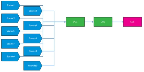
se-lected. We anonymize the networks of these problems so that we can display their structures. In this report we refer to the problem that is of the mixing type as the Mix problem. We display the structure of the Mix problem in

Fig-ure 2.1. The optimization variables in this problem are the input volumes of eight different raws. We call one of the technology problems the Split problem, because the optimization variables in this problem are twenty-five settings that

determine how several product flows are divided (splitted) over the network. The other technology problem we call the Tech problem. There are fifteen

optimiza-tion variables in this problem, namely the input volume of a raw and fourteen

(20)

technology settings. We display the network structures of the Split and the Tech problem in Appendix A.

Figure 2.1: Network structure of the Mix problem

We summarize some information about the three problems that we have at our availability in Table 2.1. In this table we introducen, the problem dimension. It equals the amount of optimization variables in a problem. The evaluation time

in the third column of the table denotes the approximate time it takes Diamond to evaluate one point in the solution space of the corresponding problem. This

gives an indication of the complexity of the problems and the time it takes to perform one optimization run, which consists of thousands such evaluations.

Table 2.1: Some information about the available problems

Problem type Problem name n Evaluation time

Mixing Mix problem 8 8 milliseconds

Technology Tech problem 15 18 milliseconds Split problem 25 45 milliseconds

For each of the three problems that we have at our availability, only one instance is defined. Other instances of the problems arise when an alteration

is made in a problem. Examples of such alterations are price fluctuations and changes in the product specifications of a certain raw or sale due to governmental

(21)

2.2. Differential Evolution 11

the transfer functions defining the processing step that takes place in a certain unit operation might require alteration, for example when a piece of machinery

is replaced by a slightly different one or when research points out that there is a better formula to describe a certain chemical process.

2.2 Differential Evolution

DE is introduced by Storn and Price (1997). It is a stochastic optimization method belonging to the class of evolutionary algorithms (EAs). EAs are meta-heuristics that incorporate mechanisms inspired by biological evolution such as

reproduction, mutation, and, recombination. The older and more widely known genetic algorithms (GAs) (Goldberg, 1989) belong to this same class. According

to some taxonomies, DE is considered a type of GA because both DE and GAs make use of a population of solutions on which selection, mutation, and crossover take place to iteratively create new population members. In both GAs and DE

the population size remains constant by discarding old members when new indi-viduals enter the population. We however are of the opinion that there are too

many characteristics setting DE apart from GAs for it to be considered one. We present these characteristics in Table 2.2. Studies focusing on the comparison of several metaheuristics indicate that GAs and other EAs are frequently

out-performed by DE (Vesterstrøm & Thomsen, 2004; Kannan, Slochanal, & Padhy, 2005; Xu & Li, 2007).

Table 2.2: Some differences that set DE apart from GAs

In a GA In DE

Selection takes place at the begin-ning of an iteration

Selection takes place at the end of an iter-ation

Two parents create two offspring in each iteration

Every parent creates one offspring in each iteration

No other population members are in-volved in creating the offspring but the two parents

Three randomly selected other population members are involved in creating the off-spring of a parent

The two offspring always replace two current population members

An offspring only replaces its parent if it corresponds to a better solution value

DE consists of two stages, an initialization stage and a main loop. In the

(22)

of Diamond is a set of feasible values for the optimization variables. With feasible we mean that the set of values yields a solution value smaller than a very large

value when it is evaluated by the evaluator. The evaluator returns this very large value when one or more of the hard constraints of the NLP resulting from the network, datastore, and optimization variables in Diamond are not satisfied.

The constraints that define the ranges of the optimization variables are hard constraints so that, for example, a negative amount of product does not become

possible anywhere in the process. All other constraints are incorporated in the objective function as soft constraints, meaning that they lead to a penalty in the objective function if, and based on the extend that, they are not satisfied.

Because of this it is possible to evaluate solutions that are actually infeasible in the current process, which has as a result that sets of feasible values can be found relatively quickly via random search and that the initialization stage of DE in

Diamond will not take long.

Although the goal in Diamond is to maximize profit, the objective function is

such that we are dealing with a minimization problem, which is also the reason for assigning infeasible solutions a very large value. In fact, the objective function is such that negative solution values correspond to profit and positive solution

values correspond to losses. Large positive solution values generally indicate unsatisfied soft constraints.

The solutions for a problem in Diamond can be represented byn-dimensional vectors in which each element represents the value selected for one of the opti-mization variables. We denote the solution value corresponding to a vector #»x in the solution space by f(#»x). f(#»x) is the output of the evaluator from Figure 1.2 when it receives the vector of values for the optimization variables #»x as input. The population size is denoted by N P. N P is one of the auxiliary

optimiza-tion parameters of DE that the user has to set a value for in Diamond before performing an optimization. After the initialization stage, a population of N P

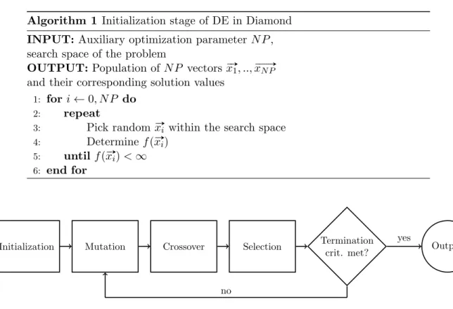
n-dimensional solution vectors have been generated. In Algorithm 1 we display pseudocode for the initialization stage of DE in Diamond. We denote the very large value that is assigned to infeasible solutions by ∞ in this algorithm.

The second and final stage of DE in Diamond is the main loop. After the initialization stage, mutation, crossover, and selection take place iteratively until

a termination criterion is met. We depict this schematically in Figure 2.2.

In the mutation step, a mutated vector is obtained for each of theN P pop-ulation members. This is done by perturbing a randomly selected poppop-ulation

(23)

mem-2.2. Differential Evolution 13

Algorithm 1 Initialization stage of DE in Diamond

INPUT:Auxiliary optimization parameterN P, search space of the problem

OUTPUT: Population ofN P vectors x# »1, ..,x# »N P

and their corresponding solution values

1: fori←0, N P do

2: repeat

3: Pick random x#»i within the search space

4: Determine f(x#»i)

5: until f(x#»i)<∞

6: end for

Initialization Mutation Crossover Selection Termination

crit. met? Output

no

yes

Figure 2.2: Schematic depiction of DE in Diamond

bers. The current population members can be seen as the parents and we hence denote them by p#»i, i = 1, .., N P. For each parent, three random other

popula-tion members are selected. If we letr1,r2, andr3 be distinct random integers in

the set {1,2, .., N P} \i, we can denote the three population members that are randomly selected for parent vector p#»i by x# »r1(i),x# »r2(i), and x# »r3(i).

The mutant vector m# »i belonging to parent vector p#»i is constructed via the

equation m# »i = x# »r1(i)+F ·(x# »r2(i)−x# »r3(i)). The parent vector is not explicitly taken into account in the construction of its corresponding mutant vector except

for that it cannot be one of the randomly selected population members. In the mutation step, another auxiliary optimization parameter of DE is introduced, the mutation factor F. According to Storn and Price (1997), F has to be in the

range [0,2]. We visualize the creation of a mutant vector in a two-dimensional problem space in Figure 2.3. In this figure, the black dots represent the current population members and the grey dot represents the mutant vector.

After the mutation step there are N P mutant vectors, one for each current

population member. Now the crossover step takes place. In this step N P new solution vectors are generated. These solution vectors can be seen as the children

(24)

optimization variable 1

optimization

v

ariable

2

# »

xr2(i)

# »

xr3(i)

# »

xr1(i)

# »

mi=x# »r1(i)+F ·(x# »r2(i)−x# »r3(i))

F ·(x# »r2(i)−x# »r3(i))

Figure 2.3: The mutation step illustrated for a 2-dimensional problem

For the construction of the child c#»i, its parent p#»i and the corresponding mutant

vectorm# »i are used. Each vector element of the child c#»i is either copied from the

parent vector p#»i or from the corresponding mutant vector m# »i. In the crossover

step another auxiliary optimization parameter of DE is introduced, the crossover

constant CR. CR influences how many of the vector elements of a child on average originate from its parent and how many on average originate from the corresponding mutant vector. CR has to be in the range [0,1]. We visualize the

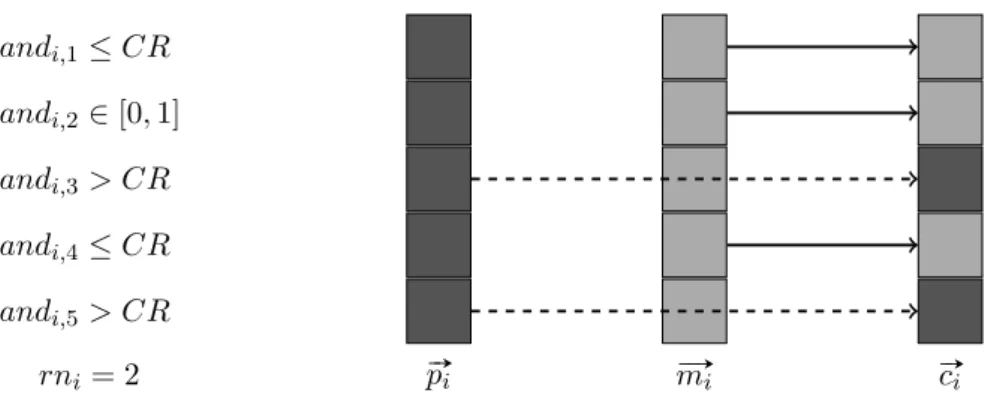
idea behind the crossover step in Figure 2.4. In this figure it can be seen how a child c#»i is constructed with the vector elements of its parent p#»i and the vector

elements of the mutantm# »i.

randi,1≤CR

randi,2∈[0,1] randi,3> CR

randi,4≤CR

randi,5> CR

rni = 2 p#»i m# »i c#»i

Figure 2.4: The crossover step illustrated for a 5-dimensional problem

(25)

2.2. Differential Evolution 15

drawn from the interval [0,1] and one random integer is drawn from the set {1,2, .., n}. We denote these numbers by randi,j,j = 1, .., nand rni respectively.

If randi,j is larger than the constant CR, the jth element of the child vector c#»i

is similar to thejth element of the vector of its parentp#»i. If this is not the case,

thejth _{element of the child vector} _c#»

i is similar to the jth element of the mutant

vector m# »i. The rnith element of the child vector c#»i is always similar to the jth

element of the mutant vector m# »i. This is to ensure that c#»i differs fromp#»i in at

least one element. In Figure 2.4, the relevant values of the random numbers that are drawn are denoted to the left of the figure.

After the crossover step all mutant vectors are discarded, leaving us withN P

parents (the current population) and N P children, each child belonging to one parent. Recall that the population members of DE in Diamond aren-dimensional

vectors that each represent a set of values for the optimization variables in the problem that is being optimized by Diamond. Because of this, each population member corresponds to a solution value. The solution values of the children

are evaluated and if the solution value corresponding to a child is better than the one corresponding to its parent, the child replaces its parent in the current population. This is the selection step. It marks the end of an iteration.

The idea behind DE is that through mutation, crossover, and selection, the population will hopefully become more and more concentrated around local

op-tima and eventually concentrate itself around the global one or global ones. De-pending on the values selected for the auxiliary optimization parameters and the specific problem at hand though, DE might converge too quickly and thus end

up in a local optimum or not convergence and thus end up in no optimum at all1 (Locatelli & Vasile, 2014). Other values can lead to very slow convergence

and are hence unable to provide the user with a good solution within a reason-able time limit or number of function evaluations. Finding proper values for the auxiliary optimization parameters for the problem at hand is therefore essential.

This process is known as tuning. We deal with tuning in Chapter 3.

In Algorithm 2, we display pseudocode for DE in Diamond. In line 3 of this

algorithm, we refer to a termination criterion. In the current situation this termi-nation criterion can either be a manual stop, a maximum number of iterations, or a maximum number of iterations without change in the solution value

cor-responding to the best-encountered solution #»y. This means that users have to decide when to stop the algorithm or select a value for either the maximum

num-1

(26)

ber of iterations or the maximum number of iterations without change, which is not in line with FC’s desire that no decisions concerning auxiliary optimization

settings have to be made by the user.

Algorithm 2 DE in Diamond

INPUT:Auxiliary optimization parameters N P,F, and CR, search space of the problem

OUTPUT: Best-encountered solution #»y

1: Initialization (see Algorithm 1)

2: #»y ←(x#»i corresponding to lowest f(x#»i) of Algorithm 1)

3: while Termination criterion not metdo

4: fori←0, N P do

5: Perform mutation and crossover to obtain child c#»i ofx#»i

6: Determine f(c#»i)

7: if f(c#»i)< f(x#»i) then ▷ Selection

8: x#»i ←c#»i

9: if f(x#»i)< f(y#»i) then ▷Update best

10: #»y ←x#»i

11: end if

12: end if

13: end for

14: end while

We restrict the software to the termination criterion of a maximum number of iterations such that a limited amount of function evaluations is performed in

one optimization run. A termination criterion based on a maximum number of function evaluations makes sense from a practical perspective. This way, users

can easily be informed of the approximate runtime that is left until termination and there is a possibility to reproduce results on different PC’s2. We only count the evaluations of points satisfying all hard constraints towards reaching the

maximum number of function evaluations. The hard constraints define the ranges of the optimization variables and if one of them is not satisfied, the evaluator immediately returns a very large value. The time this takes is negligible compared

to the time it takes the evaluator to evaluate a point in the search space of the problem that does not violate the ranges of the optimization variables. Different

optimization runs on the same problem can therefore only vary little in runtime as long as the computation environment remains unchanged. The maximum number of function evaluations (resulting in a feasible solution) can be seen as another

auxiliary parameter of DE in Diamond. In this report we refer to it as E.

2_{Because of DE’s stochasticity, results cannot exactly be reproduced unless the same random}

(27)

2.3. Conclusions on Current Situation 17

2.3 Conclusions on Current Situation

We have three problems at our availability that we briefly discuss in Section

2.1. One of those problems is of the mixing type and the other two are of the technology type. A new problem instance is created when an alteration is made

to an existing problem. In Section 2.2 we describe how DE works. DE is a stochastic optimization method that makes use of a population of solutions in the search space of a problem on which mutation, crossover, and selection take

place such that the population hopefully converges in the direction of the global optimum. Like all metaheuristics, DE’s effectiveness and efficiency depend on the

values of several auxiliary optimization parameters. The auxiliary optimization parameters of DE are the population size N P, the mutation factor F, and the crossover constant CR. The maximum number of function evaluations E can

(28)

(29)

Chapter 3 Literature Review

In this chapter we describe the literature relevant to the process of tuning

auxil-iary optimization parameters. The focus is on tuning the auxilauxil-iary optimization parameters of DE. We describe different tuning approaches in Section 3.1. One of the approaches is meta-optimization, which requires the selection of a meta-level

optimizer. In Section 3.2 we review different meta-level optimizers. We conclude this chapter in Section 3.3.

3.1 Tuning Auxiliary Optimization Parameters

Because FC would like to see that no decisions concerning auxiliary optimization settings have to be made by the user, the auxiliary optimization parameters need to be tuned for DE in Diamond. Even though tuning is crucial to metaheuristic

optimization both in academic research and for practical applications, only lim-ited research has been devoted to it (Birattari, 2009). There are three different

ways in which parameter tuning can be done, namely parameter selection, online parameter initialization, and offline parameter initialization.

Parameter selection involves selecting values for the auxiliary optimization parameters relying on conventions and default values. A default set of parameters however might lead to satisfying results on some problems but can fail to yield

good results on other problems. Parameter selection is therefore generally not a good tuning strategy. In practice though it is often applied.

Online parameter initialization is also referred to as parameter control. It in-volves changing the parameter values during the search. The following approaches

can be distinguished in the field of online parameter initialization:

• Deterministic parameter control: Random or deterministic changes in

pa-rameter values are made at predefined moments, meaning that the progress of the search is not taken into account. A deterministic parameter control

strategy that has been used in combination with DE is steadily decreasing

(30)

the crossover constantCR as the number of performed iterations increases (Mezura-Montes & Palomeque-Ortiz, 2009).

• Adaptive parameter control: Feedback from the search progress is used to

control the values of the auxiliary optimization parameters. An adaptive parameter control strategy that has been used in combination with DE is selecting a value for the mutation factor based on the relative difference

between the solution values corresponding to the best and worst population members (Ali & T¨orn, 2004).

• Self-adaptive parameter control: This can be seen as a subclass of adaptive

parameter control. In self-adaptive parameter control, each member of the population has an individual auxiliary optimization parameter for a certain step that evolves during the search. Self-adaptive parameter control

strategies for DE would involve replacing F by an N P-dimensional vector ofFis or replacingCRby anN P-dimensional vector ofCRis such that each

population member corresponds to their own mutation factor or crossover constant. Fis or CRis that did not lead to the generation of good trial

vectors during a part of the search can then be replaced by otherFis orCRis

that did lead to the generation of good trial vectors or by randomly selected other values within a certain range (Brest, Greiner, Boskovic, Mernik, &

Zumer, 2006).

There are quite a few DE adaptations that make use of online parameter

ini-tialization (Das & Suganthan, 2011). None of these seem promising for Diamond though: online parameter initialization approaches usually introduce new

auxil-iary optimization parameters whose values the user must decide upon. Further-more, experiments have shown that there is no general or consistent advantage to using online parameter initialization in combination with DE as opposed to

using classical DE with good parameters (Pedersen, 2010).

In offline parameter initialization, the values of the different auxiliary

param-eters are fixed before the start of an optimization run instead of updated during the execution of the run. The following approaches can be distinguished within

the field of offline parameter initialization:

• Manual tuning: This is also referred to as experimentational tuning. It

involves trying a default set of values for the auxiliary parameters and based on the results thereof trying a new set of values (Talbi, 2009). This process

(31)

3.1. Tuning Auxiliary Optimization Parameters 21

found. Manual tuning is a widely applied tuning strategy for metaheuristics but it is not a feasible approach for Diamond since manual tuning requires

a lot of input from the user and is hence a time consuming approach, even if the user is familiar with the optimization method (Adenso-Diaz & Laguna, 2006).

• Design of experiments: Performing a design of experiments (DOE) can

over-come the problems involved with manual tuning (Box, Hunter, & Hunter, 2005). In tuning parameters with a DOE, each auxiliary parameter is as-signed a number of values. These values can be selected randomly or via a

specific procedure such as Latin hypercube sampling (McKay, Beckman, & Conover, 1979). All combinations of the values for the different auxiliary

parameters are then evaluated several times to give an indication of how well each combination of values performs1. The number of values for each variable cannot be too small because in that case the best-encountered

aux-iliary optimization setting might not be as close to the optimal settings as one would like them to be and hence not yield satisfactory results on the

actual problems. A large number of values leads to a very large number of experiments though, which is a drawback of performing a DOE. DOE is a popular method to determine auxiliary parameters for an algorithm,

especially when the actual problems are theoretical functions that do not require much evaluation time. In Diamond though, the computation time of each experiment can be large, making DOE a less suitable approach.

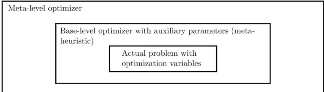
• Meta-optimization: The search for the best auxiliary optimization settings

of a metaheuristic can be treated as an optimization problem in its own right. Dealing with this optimization problem defines the concept of meta-optimization. In this concept, a black-box optimization method is used

as an overlaying meta-optimizer for finding good auxiliary optimization pa-rameters for another optimization method which in turn is used to optimize

the actual problem (Pedersen, 2010). We portray this concept graphically in Figure 3.1. With an effective and efficient meta-optimizer, a near-optimal set of auxiliary optimization parameters for another optimization method

for a specific problem can be obtained. As opposed to performing a DOE, meta-optimization requires the evaluation of only a small number of values

for the auxiliary parameters, provided that an efficient meta-optimizer has

1

(32)

been selected. We review different meta-optimizers in Section 3.2.

Actual problem with optimization variables

Base-level optimizer with auxiliary parameters (meta-heuristic)

Meta-level optimizer

Figure 3.1: The concept of meta-optimization, based on Pedersen (2010)

3.2 Meta-level Optimizers

We have identified three approaches within the field of offline parameter

initial-ization. These approaches are parameter selection, DOE, and meta-optimization, which requires the implementation of a meta-optimizer. In this section we review

different meta-optimizers. We distinguish the following three types:

• Metaheuristics: Since it is difficult to make assumptions about the search

spaces resulting from varying the auxiliary optimization parameters of a base-level algorithm, a metaheuristic is typically used as overlaying

meta-optimizer (B¨ack, 1994; Cortez, Rocha, & Neves, 2001; Meissner, Schmuker, & Schneider, 2006). The auxiliary optimization parameters of DE have been meta-optimized with a metaheuristic by Neum¨uller, Wagner, Kronberger,

and Affenzeller (2012), who use a GA as meta-optimizer but restrict their research to only one specific test function. Using a metaheuristic as

meta-optimizer has a considerable drawback. As we have explained before, all metaheuristics require the setting of auxiliary optimization parameters for them to be effective and efficient. This is what makes them so generally

applicable. Following the outlines of Section 3.1, one would find that the best approach to obtain good auxiliary parameters for the metaheuristic that is implemented as optimizer would be to implement a

meta-meta-optimization method. But where does this stop? We would hence like to find a meta-optimization method that does not require the setting

(33)

3.2. Meta-level Optimizers 23

• Race algorithms: Racing involves iteratively evaluating several possible

auxiliary parameter settings and discarding a setting as soon as sufficient

statistical evidence is gathered against it. Because of this, racing works best for base-level algorithms that have low stochasticity. Race algorithms are originally invented as a way to reduce the amount of experiments that

need to be done when performing a full factorial experiment or other type of DOE (Maron & Moore, 1994; Birattari, 2002). Because of this, all

aux-iliary parameter combinations that are evaluated need to be fixed in the initialization phase of a race algorithm. This however has as result that the optimal settings resulting from racing might not be as close to optimal as

one would like them to be since only a limited amount of auxiliary param-eter combinations can be selected. Race algorithms can be adapted though

by generating a new possible auxiliary parameter setting as soon as another setting is discarded (Van Dijk, Mes, Schutten, & Gromicho, 2014). This approach brings performing a DOE and doing meta-optimization together

by turning racing into a (guideline for constructing a) population-based meta-optimizer. For deterministic2 or low-stochastic base-level algorithms, racing is probably the best way to go. The same goes for base-level

algo-rithms depending on categorical parameters because, since racing is based on performing a DOE, it can easily deal with those as well.

• Classical direct search methods: Recently, some classical direct search

meth-ods have been implemented as meta-optimizers. Classical direct search

methods are relatively intuitive optimization methods, stemming from the beginning of the digital age, that were invented for optimizing one- or

few-dimensional functions without requiring any knowledge about the gradient of the function that is being optimized (Lewis, Torczon, & Trosset, 2000). Such methods have fallen out of favour with the mathematical optimization

community by the early 1970s because they lacked coherent mathematical analysis but are still used in some practical applications (Kolda, Lewis, &

Torczon, 2003). Although not at all competitive with metaheuristics on most types of problems, classical direct search methods are generally able to quickly locate satisfactory solutions in low-dimensional search spaces and

do not require the setting of auxiliary optimization parameters, omitting the need for tuning. This makes them well suitable for

meta-optimization in practice, provided that the base-level algorithm does not

2_{In this case multiple problem instances have to be defined and the stochastic component is}

(34)

have many auxiliary optimization parameters. Three well-known classi-cal direct search methods that use only function evaluations to search for

the optimum are the Hooke-Jeeves (HJ) method, the Nelder-Mead (NM) method, and the Luus-Jaakola (LJ) method (Armaou & Kevrekidis, 2005). We briefly review each of those.

The HJ method

The HJ method (Hooke & Jeeves, 1961), also known as pattern search, has been

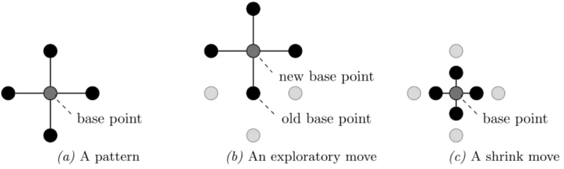
implemented as meta-level optimizer for several base-level algorithms (Cohen & Meyer, 2011; Gao et al., 2012). The method considers 2n points in the search space that lie around one randomly selected base point in a pattern such that

each of those 2npoints is equally far away from the base point and differs from the base point in only one of the variables that make up the search space. We

depict a two-dimensional pattern that follows those rules in Figure 3.2a. In meta-optimization, the variables that make up the search space are the auxiliary parameters of the base-level optimizer.

base point

new base point

(a) A pattern

old base point new base point

(b)An exploratory move

base point

new base point

(c)A shrink move

Figure 3.2: A pattern and its movements in a two-dimensional search space

This pattern is iteratively moved across the search space or shrunk towards

its base point so that hopefully the global optimum is more and more closely approximated as the iterations pass. In each iteration, the points surrounding

the base point are evaluated and the one corresponding to the best solution value becomes the new base point, provided that this solution value is better than the one corresponding to the current base point. This is an exploratory move,

which we visualize in Figure 3.2b. If none of the solution values corresponding to the surrounding points are better than the one corresponding to the base point, the base point remains unchanged and in the following iteration 2n new points

surrounding the same base point are evaluated. Those new surrounding points are located half as far away from the base point as those in the previous iteration.

(35)

after either an exploratory or a shrink move has been performed. We construct pseudocode for the HJ method and display it in Algorithm 3.

Algorithm 3 The HJ method for a minimization problem

INPUT:Search space of the problem

OUTPUT: Best-found position in the search spaceP

1: Pick initial pattern size based on search space

2: Pick random base point P in the search space

3: y←f(P)

4: whileTermination criterion not met do

5: SHRINK ← TRUE

6: for j←1,2ndo

7: Determine surrounding point Pj

8: if f(Pj)< y then

9: P ←Pj

10: y ←f(Pj)

11: SHRINK ← FALSE

12: end if

13: end for

14: if SHRINKthen

15: Shrink pattern to half its size

16: end if

17: end while

The NM method

The NM method (Nelder & Mead, 1965) is one of the most popular classical direct

search methods because of its nice analogy with geometry and its ability to quickly locate an optimum by making use of the structure of the search space (Wright,

2012). It appears though that the NM method has not been implemented as meta-optimization method. This might be due to it being more difficult to understand and implement, or to it being more likely to get stuck in local optima compared

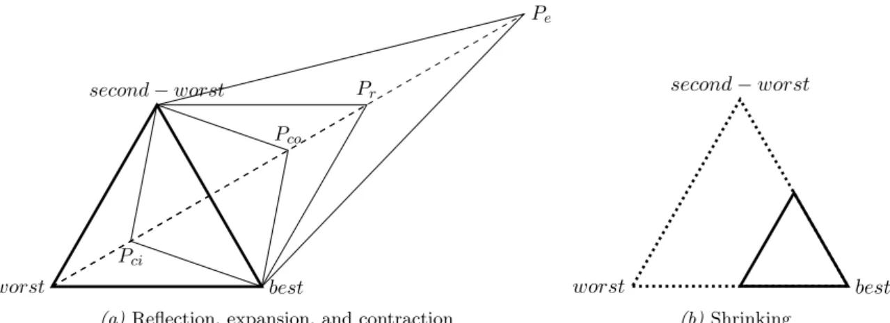
to other classical direct search methods. The method considers the vertices of an

n-dimensional simplex that iteratively moves through the search space, hopefully

in the direction of the global optimum. An n-dimensional simplex consists of

n+ 1 vertices, each connected with one another. A one-dimensional simplex is a line segment and a dimensional simplex is a triangle. We depict a

two-dimensional simplex and the movements it can perform in the NM method in Figure 3.3.

The idea behind the NM method is to update the simplex in each iteration by replacing the worst vertex with a more promising one or to shrink the simplex

(36)

worst best

second−worst Pr

Pe

Pci

Pco

(a)Reflection, expansion, and contraction

worst best second−worst

(b)Shrinking

Figure 3.3: A simplex and its movements in a two-dimensional search space

from the worst vertex so that point Pr is created, see Figure 3.3a. Pr replaces

the worst vertex if it corresponds to a better solution value than the

second-worst vertex. This leads to an updated simplex and ends the iteration unless Pr

corresponds to a better solution value than the best vertex. In that case, the

simplex is expanded and point Pe is created, see Figure 3.3a. Pr is replaced by

Pe if Pe corresponds to an even better solution value. This then marks the end

of the iteration.

IfPr did not replace the worst vertex, implying that it did not correspond to

a better solution value than the second-worst vertex and hence did not lead to an updated simplex, a contraction is performed. This can either be an outside

con-traction yielding pointPcoor an inside contraction yielding point Pci, see Figure

3.3a. An outside contraction is performed if Pr corresponds to a better solution

value than the worst vertex and an inside contraction is performed if this is not

the case. The contracted point replaces the worst vertex if it corresponds to a better solution value, leading to an updated simplex and ending the iteration. If

the contracted point does not correspond to a better solution value, the simplex is shrunk towards the best vertex such thatnnew vertices are created, see Figure 3.3b. We construct pseudocode for the NM method and display it in Algorithm

4. We also create a flowchart for the NM method which is more detailed than the pseudocode. We refer the interested reader to Appendix B.

The LJ method

The LJ method (Luus & Jaakola, 1973) has been implemented as meta-level optimizer for several base-level algorithms (Rychlicki-Kicior & Stasiak, 2014;

(37)

Algorithm 4 The NM method for a minimization problem

OUTPUT: Best-found position in the search spacePn

1: Pickn+ 1 random points in the search space: P0, P1, .., Pn

2: Order points such that f(P0)> f(P1)>··> f(Pn)

3: whileTermination criterion not met do

4: Reflection to obtain point Pr

5: if f(Pr)< f(P1) then

6: P0 ←Pr

7: if f(Pr)< f(Pn) then

8: Expansion to obtain point Pe

9: if f(Pe)< f(Pr)then

10: Pr←Pe

11: end if

12: end if

13: else

14: if f(Pr)< f(P0)then

15: Outside contraction to obtain point Pc

16: else

17: Inside contraction to obtain point Pc

18: end if

19: if f(Pc)< f(P0) then

20: P0 ←Pc

21: else

22: Shrink towards point Pn

23: end if

24: end if

25: Order points such that f(P0)> f(P1)>··> f(Pn)

26: end while

DE have been meta-optimized with Local Unimodal Sampling (LUS) (Pedersen & Chipperfield, 2008), a minor adaptation of the LJ method, by Pedersen (2010).

The LJ method starts with the selection of a random point in the search space. We refer to this point as the current point. In each iteration, a random point is selected from a range and added to the current point. This range is initially

equal to the range of the search space. If the point resulting from the addition corresponds to a better solution value than the current point, it replaces the cur-rent point. The search range is then re-centred around the curcur-rent point and the

iteration is finished. If the point resulting from the addition does not correspond to a better solution value than the current point, the search range from which

(38)

unchanged. Because the search range is always re-centred around the current point, it can extend over the boundaries of the search space. If a point is drawn

inside the search range that does not lie inside the search space, it is discarded and a new point is drawn without decreasing the search range. We construct pseudocode for the LJ method and display it in Algorithm 5.

Algorithm 5 The LJ method for a minimization problem

OUTPUT: Best-found position in the search spaceP

1: Pick random pointP in the search space

2: Set search range equal to search space

3: while Termination criterion not metdo

4: Pick random pointPr in search range

5: Pn←P+Pr

6: if f(Pn)< f(P) then

7: P ←Pn

8: Re-centre search range aroundP

9: else

10: Decrease search range by a factor 0.95 in each direction

11: end if

12: end while

LUS differs from the LJ method in the sense that the factor 0.95 used to

decrease the search range in line 9 of the algorithm is replaced by (1_/₂₎1/3n_{. This} adaptation of the original LJ method has as a result that the method is able

to more quickly locate near-optimal solutions in low-dimensional search spaces and is less likely to converge to non-optimal solutions in high-dimensional search spaces.

3.3 Conclusions on Literature Review

In Section 3.1 we discuss several approaches for auxiliary parameter tuning. These approaches are parameter selection, online parameter initialization, and offline

parameter initialization. One form of offline parameter initialization is meta-optimization, which requires the implementation of a meta-optimizer. We review several types of meta-optimizers in Section 3.2, namely metaheuristics, race

(39)

Chapter 4 Solution Approach

In Chapter 3 we have discussed several approaches for tuning auxiliary

optimiza-tion parameters. We select a tuning strategy for DE in Diamond in Secoptimiza-tion 4.1 and determine our solution approach this way. In Section 4.2 we construct a flowchart of the new situation in Diamond. We conclude this chapter in Section

4.3.

4.1 Tuning in Diamond

The approaches for tuning auxiliary optimization parameters that we have dis-cussed in Chapter 3 are parameter selection, online parameter initialization, and

offline parameter initialization. We discuss the applicability of parameter selec-tion to Diamond in Secselec-tion 4.1.1 and the applicability of offline parameter

initial-ization to Diamond in Section 4.1.2. Online parameter initialinitial-ization approaches usually introduce new auxiliary optimization parameters whose values the user must decide upon, worsening the problem that decisions concerning auxiliary

op-timization settings have to be made by the user. Online parameter initialization does therefore not seem promising in the context of Diamond.

4.1.1 Parameter Selection in Diamond

Parameter selection is the simplest tuning approach. It involves selecting values for the auxiliary optimization parameters relying on conventions and default

val-ues. Parameter selection is generally not a good tuning strategy since a default set of parameters might lead to satisfying results on some problems but can fail to yield good results on other problems. However, due to its simplicity, parameter

selection is a preferred approach when it can yield good results.

In Chapter 2 we have identified four auxiliary parameters in Diamond that

require tuning: the population size N P, the mutation factor F, the crossover constant CR, and the maximum number of function evaluations E. Some

con-ventions and default values regarding DE’s auxiliary optimization parameters

(40)

N P, F, and CR can be found in literature. We summarize these in Table 4.1. We base the required ranges in this table on Storn and Price (1997) and the

common ranges and values on Storn and Price (1997), Lampinen et al. (2005), R¨onkk¨onen, Kukkonen, and Price (2005), and Talbi (2009).

Table 4.1: The three auxiliary optimization parameters of DE

Parameter Required range Common range Common value

N P {4,5, ...} {5n,5n+ 1, ..,10n} ⌈7.5n⌉ †

F [0,2] [0.4,1] 0.7 †

CR [0,1] {[0,0.2],[0.8,1]} 0.9

† _{Due to lack of consensus on a proper default value for this}

pa-rameter, we select the midpoint of its common range.

Although good values forN P andF depend on the problem at hand, on the runtime, and on each other’s value, a value of 0.9 appears to be near-optimal for

CRin a wide variety of problems, independent of the values selected forN P and

F and the runtime, and is therefore generally advised in literature (R¨onkk¨onen et al., 2005; Montgomery, 2009; Talbi, 2009). CR ∈ [0,0.2] has been shown

to be effective for quite a lot of problems as well and on those problems more efficient thanCR= 0.9, but research has pointed out that the problems on which

CR∈[0,0.2] is effective and efficient are all separable functions1(Lampinen et al., 2005; R¨onkk¨onen et al., 2005). Lots of theoretical test and benchmark functions are separable but the problems in Diamond are definitely not. We can thus

apply parameter selection to the auxiliary optimization parameterCRby setting

CR = 0.9 as default value, and tune the auxiliary optimization parameters N P

and F using a different approach.

We also apply parameter selection to the fourth auxiliary parameter of DE in Diamond, the maximum number of function evaluations E. This is because a

larger maximum number of function evaluations generally leads to a better solu-tion value but also to more computasolu-tion time. We have to cut it off somewhere. We decide to terminate the algorithm as soon as 1500·n function evaluations

resulting in a feasible solution value have been performed,nbeing the amount of optimization variables of the problem. Because a number of function evaluations

much larger than 1500nis generally required to obtain good solution values with DE, we make sure that our solution approach is such that the maximum number

1_{Separable functions are functions depending on multiple variables that can be represented}

(41)

4.1. Tuning in Diamond 31

of function evaluations can be altered if desired in practice or in further research.

4.1.2 Offline Parameter Initialization in Diamond

Recall from Chapter 3 that the field of offline parameter initialization can be subdivided in the fields of manual tuning, DOE, and meta-optimization. Manual

tuning is not a promising approach for Diamond because it requires a lot of input from the user. Performing a DOE and applying meta-optimization make it

possible to search for good auxiliary DE parameters for a certain problem without requiring any input from the user during the search. No input from the user is required before the search either (except of course for a datastore, a network, and

optimization variables), provided that the method for determining the auxiliary parameter values on which the DOE is performed or the optimizer implemented at the meta-level is parameter-free.

Both performing a DOE with a parameter-free method for determining the auxiliary parameter values on which the DOE is performed and applying

meta-optimization with a parameter-free meta-level optimizer are promising approaches for Diamond. They can tackle the problem that we have identified in Chapter 1. Meta-optimization has the advantage over DOE that less combinations of values

for the auxiliary optimization parameters have to be evaluated, provided that a good meta-optimizer has been selected, which can result in better solutions

and large computational time savings. We therefore select meta-optimization in our solution approach as the tuning strategy for DE’s auxiliary optimization parameters N P and F.

Meta-optimization requires the implementation of a meta-level optimizer, which we want to be parameter-free. To decide upon the optimization method that we implement as meta-level optimizer, we introduce the concept of meta-level

search spaces. Just like the problems in Diamond induce search spaces resulting from varying the optimization variables, the meta-optimization problems in

Di-amond induce search spaces resulting from varying DE’s auxiliary optimization parameters. We call the search spaces that result from varying N P and F the meta-level search spaces of Diamond.

We can examine the meta-level search spaces in Diamond with the creation of 3-D plots. This can help us in selecting an effective and efficient meta-level optimizer. To examine the meta-level search space of a problem in Diamond, we

perform a DOE with grid search. In a grid search each auxiliary optimization parameter is assigned a range. These ranges are split up in equally sized intervals

(42)

in performing the DOE. In two dimensions the combinations of values can easily be visualized as a grid, hence the name. As we have explained in Chapter 3,

performing a DOE is a computationally time expensive task. We hence only examine the meta-level search space of the Mix problem. Optimization runs on this problem take considerably less computation time than optimization runs on

the other two problems due to its smaller dimension and smaller evaluation time per point in the base-level search space (see Table 2.1).

To perform a DOE with grid search, we need to select ranges and interval sizes

for the auxiliary parameters, and decide how many times each combination of auxiliary parameter values is evaluated. The ranges for the auxiliary parameters we choose such that the common ranges of Table 4.1 are widely spanned, namely

[n,15n] forN P and [0.1,1.5] for F. We selectn as interval size for N P and 0.1 for F so that we obtain 15 values for each auxiliary parameter. We perform a

DOE by evaluating each combination of values 25 times to give an indication of how well each combination of values performs.

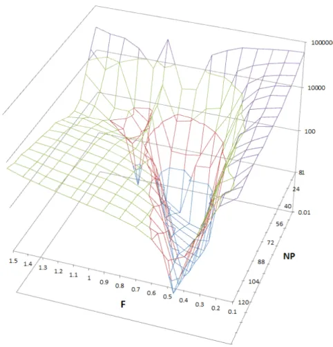
To approximate the meta-level search space of the Mix problem, we depict the average solution value resulting from each combination of auxiliary optimization

parameters in a 3-D plot. We do a log transformation on the solution values to depict the structure of the entire search space more clearly. This is necessary because there exist large differences between the average solution values resulting

from different auxiliary parameter settings due to a large amount of penalized soft constraints that can be far from satisfied in some optimization runs. Because

solution values indicating profit are negative and log transformation are impossi-ble on negative values, we subtract the lowest solution value of all solution values prior to the log transformation. The resulting plot is an approximation of the

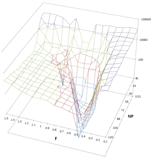
meta-level search space of the Mix problem. We depict it in Figure 4.1.

We learn from Figure 4.1 that the meta-level search space of the Mix problem is likely nearly bimodal. With bimodal we mean that there are only two optima in

the search space. Of these optima one is located on either side of the discontinuity atF = 1. The discontinuation around F = 1 can be explained by inspecting the mutation step. Recall from Chapter 2 that mutation is performed using the

equation m# »i =x# »r1(i)+F ·(x# »r2(i)−x# »r3(i)), i= 1, .., N P. For F = 1, x# »r1(i)+F · (x# »r2(i)−x# »r3(i)) =x# »r2(i)+F·(x# »r1(i)−x# »r3(i)). This has as a result that the offspring is slightly less diversified after each iteration when DE is performed with F = 1

compared to when DE is performed with, say,F = 0.95 orF = 1.05. Apparently, after a large amount of iterations, this effect becomes quite a problem, especially

(43)

4.1. Tuning in Diamond 33

Figure 4.1: Approximation of the meta-level search space of the Mix problem

If we assume that the meta-level search space of the Mix problem is somewhat

representative for all Diamond’s meta-level search spaces resulting from varying DE’s auxiliary optimization parameters N P and F, the NM method seems to be the most promising meta-level optimizer for Diamond. This is because the

meta-level search space of the Mix problem appears to be near-unimodal2, with statistical noise, as long as either F ∈[0,1] or F ∈[1,2]. We state in Chapter 3

that it appears that the NM method has not been implemented as meta-optimizer thus far and that this might be due to the fact that it is more likely to get stuck in local optima compared to other classical direct search methods. This is not a

problem though if our assumption of near-unimodality of the meta-level search spaces resulting from varying DE’s auxiliary optimization parameters N P and

F is correct. It is in fact advantageous if the assumption is correct, because the

2