The evolution of shear bands under rapid drawdown conditions in variably permeable porous soils

Full text

(1)The evolution of shear bands under rapid drawdown conditions in variably permeable porous soils. Author: W.H. Pater Supervisors: Dr. U.F.A. Karim, Dr. M.S. Krol Date: 12-05-2016.

(2) 2. Acknowledgement Many thanks go out to Dr. Sam Karim and Dr. Maarten Krol for their patience and support. I would also like to thank Inte Dessing for supporting me..

(3) 3. Table of content Acknowledgement ........................................................................................................................................ 2 Table of content ............................................................................................................................................ 3 List of figures ................................................................................................................................................. 4 List of tables .................................................................................................................................................. 4 List of algorithms ........................................................................................................................................... 4 Notation (bolt is the tensor notation) ............................................................................................................ 5 Abstract ........................................................................................................................................................ 7 1. Introduction .............................................................................................................................................. 8 2. Model formulation .................................................................................................................................. 10 2.1 global FE equations ................................................................................................................................ 10 2.2 local FE equations .................................................................................................................................. 13 3. RDD simulation of partially immersed levees & element analysis ............................................................ 17 3.1 Random permeability field simulator ........................................................................................................ 17 3.2 Large scale RDD simulation ....................................................................................................................... 18 3.3 Shear band simulation ............................................................................................................................... 24 3.4 Shear bands results with the RFEM ........................................................................................................... 25 3.5 numerical difficulties ................................................................................................................................. 33 4 Concluding remarks .................................................................................................................................. 35 4.1 conclusion .................................................................................................................................................. 35 4.2 further research ......................................................................................................................................... 35 Reference .................................................................................................................................................... 37 Appendix A: additional results for a different random permeability field .................................................... 39 Appendix B: derivatives for Newton solver global and local equations ........................................................ 44 Appendix C: Matlab program ....................................................................................................................... 47.

(4) 4. List of figures Figure 1 LAS algorithm: (a) initial random mesh; (b) refined random mesh .......................... 18 Figure 2: FEM mesh element scale simulation: (a) random permeability field; (b) mesh and BC ................................................................................................................................... 20 Figure 3 Development of porewater pressure: (a) initial phase; (b) RDD phase ................... 21 Figure 4 RDD: suction regions of interest for element scale simulation ................................ 22 Figure 5: histogram with the distribution of suction after 1000 RDD Monte Carlo simulations ........................................................................................................................................ 23 Figure 6 FEM mesh element scale simulation: (a) random permeability field; (b) mesh and BC ................................................................................................................................... 25 Figure 7 degree of saturation: (a) 25 % compression; (b) 50% compression; (c) 75% compression; (d) 100% compression ............................................................................. 27 Figure 8 deformation (gradient): (a) 25 % compression; (b) 50% compression; (c) 75% compression; (d) 100% compression ............................................................................. 28 Figure 9 volumetric strain invariant: (a) 25 % compression; (b) 50% compression; (c) 75% compression; (d) 100% compression ............................................................................. 30 Figure 10 stress ratio –q/p: (a) 25 % compression; (b) 50% compression; (c) 75% compression; (d) 100% compression ............................................................................. 31 Figure 11 deviatoric strain invariant: (a) 25 % compression; (b) 50% compression; (c) 75% compression; (d) 100% compression ............................................................................. 32 Figure 12 degree of saturation 2nd field: (a) 25 % compression; (b) 50% compression; (c) 75% compression; (d) 100% compression ............................................................................. 39 Figure 13 deformation (gradient) 2nd field: (a) 25 % compression; (b) 50% compression; (c) 75% compression; (d) 100% compression ...................................................................... 40 Figure 14 volumetric strain invariant 2nd field: (a) 25 % compression; (b) 50% compression; (c) 75% compression; (d) 100% compression ................................................................. 41 Figure 15 stress ratio –q/p 2nd field: (a) 25 % compression; (b) 50% compression; (c) 75% compression; (d) 100% compression ............................................................................. 42 Figure 16 deviatoric strain invariant 2nd field: (a) 25 % compression; (b) 50% compression; (c) 75% compression; (d) 100% compression ...................................................................... 43. List of tables Table 1: soil parameters ......................................................................................................... 19 Table 2: soil parameters ......................................................................................................... 24. List of algorithms Box 1: steps in solving the global equations .......................................................................... 13 Box 2: steps in solving the local equations ............................................................................. 16.

(5) 5. Notation (bolt is the tensor notation) 𝑵 𝑵 𝟏. 𝛁𝒔 𝑵 𝝈 𝑆( 𝑆(,* 𝑝, 𝒖 𝑑𝐴 𝑑𝐿 𝒕 𝑆2 𝑆3 𝑠5 𝑛 𝑚 𝑝5 𝑐9 ∅; ∅5 ∅, 𝜌; 𝜌, 𝜌5 𝝂 𝑘? 𝑘; 𝑬 𝑔 𝑧 𝜺𝒆 𝜺𝒕𝒓 ∆𝜆 𝐺 𝐹 𝐼2 𝐼3 𝐼L 𝐽3 𝐽L 𝑝’ 𝑞 𝑡 𝛿. shape function tensor (displacement) [] shape function tensor (porewater pressure) [] Unit vector derivative shape tensor (displacement) [/m] stress vector [kN] degree of saturation [] degree of saturation previous time-step [] porewater pressure [kPa] displacement [m] element area [m2] element length [m] traction tensor [kPa] min. degree of saturation [] max. degree of saturation [] Van Genuchten parameter (1) [kPa] Van Genuchten parameter (2) [] Van Genuchten parameter (3) [] air pressure [kPa] capillary pressure [kPa] solid fraction [] air fraction [] water fraction [] intrinsic solid density [kg/m3] intrinsic water density [kg/m3] intrinsic air density [kg/m3] Darcy flow tensor [m/s] unsaturated permeability [] saturated permeability [m/s] derivative shape tensor (porewater pressure) [/m] gravity acceleration [m/𝑠 3 ] elevation [m] elastic strain tensor [] trial strain tensor [] plastic multiplier [] flow surface [kPa] yield surface [kPa] first tensor invariant [kPa] second sensor invariant [kPa] third tensor invariant [kPa] second deviatoric invariant [kPa] third deviatoric invariant [kPa] effective volumetric stress [kPa] deviatoric stress [kPa] lode angle [] yield surface variable [].

(6) 6 𝑒 𝑝R 𝑝R,* 𝜀TU( 𝜀TV 𝜆 𝜅 𝑎 𝑏 𝑐 𝜐[ 𝑐2 𝑐3 𝑓(𝑠) 𝐾 𝜇[ 𝐂 ∆𝑡 𝑝R 𝜀; 𝑹 U 𝒅𝑹. 𝒅𝑼. 𝜇e 𝜎e 𝜃e 𝜇hi (e) 𝜎hi e. ellipticity parameter [] pre-consolidation pressure [kPa] pre-consolidation pressure previous time-step [kPa] volumetric strain trial [] volumetric strain elastic [] virgin compression index [] recompression index [] effective pre-consolidation variable (1) [] effective pre-consolidation variable (2) [] effective pre-consolidation variable (3) [] reference specific volume [] unsaturated fitting parameter (1) [] unsaturated fitting parameter (2) [] suction function [] Bulk modulus [kPa] Shear modulus [kPa] Stress-Strain tensor [kPa] time-step [s] effective pre-consolidation pressure [kPa] shear strain [] vector with global equations global solution vector with displacement and porewater pressure derivate matrix of the global equations Mean permeability Standard deviation Isotropic spatial correlation parameter Mean of the logarithm of permeability Standard deviation of the logarithm of permeability.

(7) 7. Abstract Rapid drawdown (RDD) is a specific slope stability problem in geo-mechanics that can be approached both deterministically and probabilistically and simulated numerically with the Finite Element Method (FEM) or Random Finite Element Method (RFEM) on Multi-scale levels. The field (large-scale) boundary problem is simulated herein with a coupled- (water flow- solid skeleton) deformation formulation, assuming an elastic medium using the Random Finite Elements Method (RFEM). This renders an assessment of the probability of a slope sliding from gravitational-, seepage- and water-boundary forces corresponding to RDD. On the pore-scale, the effect of non-homogeneity in the degree of saturation is closely studied using the RFEM on an element level. The element (small-scale) analysis however implemented an elastic-plastic constitutive relationship. These differences in simulating recoverable deformation (elastic) and irrecoverable deformation (elastic-plastic) are applied for “computational” convenience to enable running the developed algorithms for these two computationally demanding problems on a personal computer. The two analyses are inseparable however and demonstrate the promising results attainable despite the use of an “elastic” description for the large-scale slope problem. The heterogeneity that results from random permeability fields are found to strongly influence the location and magnitude of hydraulic gradients and shear stresses in both the large- and element-scale representation of an idealized partial immersed levee under RDD. Presence of such random field enhances shear bands development at local (elements) scale that might trigger levee’s (mass) collapse during or after RDD. Close-ups are shown for the evolution of shear bands of soil elements under compression and subsequent decompression conditions that are found prevalent during RDD. When considering plasticity the decrease in effective pre-consolidation pressure 𝑝R through the increased saturation drives the onset of shear bands. This is enhanced by the random permeability field and results in heterogeneity in the degrees of saturation of the soil. Elastic material descriptions do not lead to such levels of heterogeneity since (effective) preconsolidation pressure is not considered. During the subsequent decompression reaction almost instant softening and bifurcation was discovered due to reversal of strain from compression to extension in regions where prior intense shearing was present. This result is consistent with observations that material variability drives the onset and evolution of shear bands in many actual geotechnical situations. Despite promising results numerical difficulties where encountered when the momentumand mass equations where solved on the element level. These difficulties are discussed in and some suggestions are made to improve the performance of the algorithm which is used to solve the coupled elastic-plastic constitutive equations that constitute the model..

(8) 8. 1. Introduction Shear bands are a well-understood phenomenon where strain localization is concentrated in regions of intense shearing when porous materials deform. With uncoupled-, nonlinear materials where only the momentum equations are solved and not the mass equations, shear bands are triggered by material imperfections [4]. A previous study revealed how in coupled-, unsaturated material shear bands are triggered where momentum and mass equations are solved simultaneously, by creating a heterogeneous initial degree of saturation [1]. This research builds on this previous work by investigating the triggering of shear bands through randomly varying hydraulic saturated permeability during loading with a uniform initial degree of saturation. Shear bands are mostly studied under compression conditions. A research gap is the behavior of shear bands under decompression conditions. This is relevant for practical geotechnical situations such as the drawdown phenomenon. Drawdown occurs when surface water next to a partially submerged levee slope lowers. This most commonly occurs over several day’s during draughts, or several hours when flood gates and other water defense structures are opened to regulate water levels. Reduction of pore-water pressure inside a slope and the removal of a boundary pressure, which also acts as a retention force, affect the stability of the levee. Few deterministic FEM studies are found on the development of instability in levees during drawdown [5]. None to date however has tackled shear-band formation and non-uniform flow in slope stability RDD problems of nonlinear, saturated or unsaturated slopes using the coupled RFEM. There are numerous case studies of RDD problems such as in the one on the Shira dam where a coupled simulation was necessary for realistic calculation of porewater pressure and effective stresses [6]. RDD problems in the Netherlands are often cases where due to periods of flooding, retention regions are used to store the surplus of water triggering surface water fluctuations [7]. Most of these cases revolve around large scale levee systems that are subjected to rapid drawdown of several meters per hour. So far, no large scale failures are reported in the Netherlands. When RDD does impact partially submerged levees on a large scale this could have severe consequences on water management and levee remediation repairs [8]. Prior to RDD a levee is usually partially saturated and compressed for a limited time under the free river and slope surface flow-line water levels. When water pressure is subsequently removed due to falling water levels a disparity is created between porewater pressure inside the levee and external water pressure. The unsaturated region above the new phreatic surface where shear bands mostly form will increase in size. The evolution of a shear band that occurs under these locally undrained conditions is the result of the coupling between the fluid, gas and solid phase of the soil [9]. It is termed locally undrained because depending on the permeability some fluids transport will occur inside the soil while hardly any boundary flow as a result of surface water fluctuations takes place. This then can lead to unsaturated regions where negative pore pressure or suction slows down pressure dissipation in granular materials [10]. The aim of this work is to analyze and numerical simulate the evolution of shear bands triggered by a random permeability field under RDD conditions on the element level. Since the element level simulation is a small part of the.

(9) 9 levee under investigation, a field-scale simulation is needed to establish realistic state parameters and initial- and boundary conditions (BC). The scope of the numerical analysis is limited to simulating the evolution of shear bands on the element level in which the permeability of the soil is randomly distributed. The permeability parameter is selected since it affects both porewater pressure and deformation behavior of the soil. State parameters and BC intend to replicate the situation in the rapid drawdown region before bifurcations and mesh dependency occurs. To correctly model mesh dependency and bifurcation, Finite Element (FE) strain enhancement methods or variations of the extended finite element method (XFEM) is needed [11]. The macro level problem is computationally manageable and is usually of size that does not require simplifications to parameters or BC in laboratory scale samples to attain computational efficiency. Shear bands are small-scale microscopic occurrences in contrast to RDD that is on a larger-scale where an entire levee must be modelled and where often simplifying assumptions are necessary to attain numerical convergence. Due to processing power constraints RDD is simulated through assuming the soil sample is compressed on the element level until the confinement pressure fails resulting in a decompressing reaction. A randomly generated variable hydraulic permeability field will then be used to trigger shear a bands in an otherwise uniform deformation field. The results can then be projected back to the field problem although suffering from a limited elastic- material description. Thesis chapters are structured to show some essential features, analysis and solution process followed to demonstrate that shear band formation in the larger RDD problem are linked to the behavior of the elements in the maximum shear regions formed in the real problem. The FE and RFEM formulation fundamentals as well as the constitutive relationships used are shortly given in chapter 2. The evolution of shear bands is then studied by performing the elastic RFEM RDD simulation and elastic-plastic RFEM simulation in chapter 3 as well as some remarks involving the numerical difficulties in simulating shear bands with the coupled, elastic-plastic constitutive equations. In chapter 4 conclusion and future research are presented. In appendix A additional result of a simulation with a different random fields are provided as well as the derivatives of the FE formulation and a short explanation of the FE code that was developed for this research. The FE code can be downloaded from: http://www.stateoftheartengineering.nl/software/shearbandgenerator.

(10) 10. 2. Model formulation Shear bands in unsaturated porous media is a physical 3-phase coupled problem that is formulated numerical with the momentum- and mass equations so that pore pressures and displacements are simultaneously solved with the FEM at all the (global) elements’ nodes [1], [12], [24]. At (local) integration points within each element strains, stresses, degree of saturation and the constitutive elastic-plastic tangent operator are calculated using the coupled model [2]. A constitutive consistent tangent operator is the result of elastic-plastic soil deformation that couple’s stresses, strains and (unsaturated) hardening [13]. A multilevel Newton algorithm is used to solve the equations and the local equations are solved in the strain space [14]. Such formulations and their FE codes are found in details in many text books and publications and need not be repeated herein. An overview of the main steps of an iteration towards a solution is provided in box 1. The implementation is made in Matlab and starts with a mesh generator that interprets and sets the BC and then solves the assembled global system of equations at each load-step n.. 2.1 global FE equations The global (Biot) equations to solve for the global FE domain are the momentum (1) and mass equation (8). Unsaturated behavior is reflected through the degree of saturation 𝑆( and unsaturated Darcy flow 𝒗. m3. m3. 𝛁 𝒔 𝑵𝑻 𝝈 − 𝑆( 𝑝, 𝟏. 𝑑𝐴 − m2. q3. 𝑵𝑻 𝜌 𝑔 𝑑𝐴 − m2. 𝑵𝑻 𝒕 𝑑𝐿 = 0 (1) rq2. In equation (1) 𝛁 𝒔 𝑵𝑻 represents the derivative of the shape function while 𝑆( represents the degree of saturation function: 𝑆( = 𝑆2 + 𝑆3 − 𝑆2. 𝑐9 1+ 𝑠5. * tu. (2). Where 𝑆2 , 𝑆3 , 𝑠5 , n and m are fitting parameters that represent the van Genuchten relation that determine flow and water storage in the unsaturated region [10]. The capillary pressure or suction (𝑐9 ) is equal to: 𝑐9 = −𝑝,. (3). Furthermore 𝑝, stands for the porewater pressure. The symbol 𝝈 is the effective stress tensor that represent the internal stresses in the soil skeleton. The tensor 𝟏 is used to represent the unit vector that connects porewater pressure and degree of saturation to the x-, y- and z-direction effective stresses in the soil. The first part of equation (1) are the m3 equations that are attributed to internal momentum forces. The m2 𝑑𝐴 stands for the integration of the area of an element in the case of a two dimensional system..

(11) 11 The external momentum part in equation (1) are the self-weight of the soil and the external forces due to traction. The tensor 𝑵𝑻 stand for the shape function while parameters ρ and g stand for the density and gravity acceleration. Note that density will change with the degree of saturation 𝑆( : 𝜌 = 𝜌; ∅; + 𝜌5 ∅5 + 𝜌, ∅ ,. (4). ∅; , ∅5 and ∅, are the solid, air and water fractions of the mixture. Furthermore 𝜌; , 𝜌5 and 𝜌, are the intrinsic densities of the solid, air and water fraction. The solid fraction ∅; relate to porosity through: ∅; = 1 −. T{ t2 T{. (5). Where 𝑣[ stands for the ‘reference specific volume’ parameter. When porosity is known the other quantities are calculated through the degree of saturation 𝑆( through: ∅5 = 1 − S( 1 − ∅;. (6). and ∅, = S( 1 − ∅;. (7). The surface forces are calculated over the length of an element side where the external q3 force is applied in the mesh over integral rq2 𝑑𝐿 . The magnitude of the surface force is described by the tensor: 𝒕 . The second main equation to be solved in the FE mesh is the mass balance: m3. 𝑵𝒕 𝑆( 𝟏. 𝛁 𝒔 𝑵 𝑢 − 𝑢* 𝑑𝐴 … m2 m3. m3. 𝑵𝒕 1 − ∅; 𝑆( − 𝑆(,* 𝑑𝐴 − ∆𝑡. + m2. 𝑬𝒕 𝒗 𝑑𝐴 = 0 (8) m2. In formula (9) 𝑵 is the shape function associated to the porewater pressure element. Note that in many FE applications a lower order element is used for the mass balance. This is to cancel out spurious porewater pressure oscillations [11]. However, in this work the same element is chosen where a so-called polynomial pressure projection technique (ppp) is used to stabilize the equations [21]. This is further explained in chapter 3..

(12) 12. Where 𝛁 𝒔 𝑵 𝒖 − 𝒖𝒏 calculates the mass differential due to volumetric strain. Here 𝑢 stand for the displacement of an element. The underscore ‘n’ stands for previous time-step. The first part of the mass balance is thus attributed to the coupling between porewater pressure and displacement. This mirrors the momentum balance of equation (1) where porewater pressure is coupled to the effective soil stresses to form total stresses. The second part in equation (8) is also called the storage equation where the change in saturation results in a mass change and thus porewater pressure change in the element [15]. The third part is the mass transport equation where the derivative transpose of the shape function 𝑬𝒕 , time-step ∆𝑡 and the Darcy flow 𝒗 is calculate. Note that when ∆𝑡 no mass transport takes place and the equations becomes the undrained equation that covers a partially- and fully saturated medium. When saturation 𝑆( is equal to unity large part of both equation (1) and (8) disappear and the saturated Biot’s equation remain. The Darcy flow function is formulated by: 𝒗 = −𝑘? ∗. 𝑘; 0. 𝑝, 0 𝑬 +𝑧 𝑘; 𝜌, 𝑔. (9). Where 𝑘? is the unsaturated equivalent permeability and 𝑘; is the saturated permeability [1]. Since total water pressures are calculated in the current model 𝑧 represents the elevation of the element. The unsaturated modification to the permeability is calculated with the same “van Genuchten” [10] as 𝑆( : 𝑘? =. 2 𝜃3. 1− 1−. 2 u 3 u 𝜃. (10). Where theta 𝜃 stand for: 𝜃=. 𝑆( − 𝑆2 𝑆3 − 𝑆2. (11). To solve the global system of equations (1) to (11) the algorithm in Box 1 is needed, similar to the one described in [1]. In Box 1 R and the derivative of R with reference to the solution …† vector U, ( ) are formed at each iteration step for the implicit Newton solver. The Newton …‡ derivatives for the global equations are described in appendix B..

(13) 13 Step 1. Initialize: n=1, form mesh, BC, set displacement and porewater pressure vector: 𝑼𝒏 and set pre-consolidation pressure 𝑝R,* Step 2. Load-step loop: apply BC add each load-step, set 𝑼𝒏ˆ𝟏 = 𝑼𝒏 and set 𝑝R,*ˆ2‰ 9Š,‹ Step 3. Iteration loop: loop element and gauss points to form global equation vector R 𝒅𝑹 and equation derivate 𝒅𝑼 Step 4. Check at each gauss point of yield surface is crossed, if yes, go to box 2 Step 5. Newton iteration: solve 𝑼𝒏ˆ𝟏 = 𝑼𝒏ˆ𝟏 -. 𝒅𝑹 t𝟏 𝑼. Step 6. When tolerance is reached close iteration loop, and update 𝑼𝒏 and 𝑝R,* array’s, load next load-step Box 1: steps in solving the global equations. 2.2 local FE equations As was mentioned earlier, in equation (1), 𝝈 stands for the effective stresses in the soil skeleton. This stress is calculated in each stress point according to an elastic-plastic model depending on the pre-consolidation pressure, capillary pressure and the elastic strain trial. The unsaturated elastic-plastic model that was choses for this research is a generalized unsaturated general Cam-Clay model [1], [16]. These elastic-plastic equations are solved when the yield surface of box 1 is crossed and solved with the implicit algorithm of Box 2. In that case the trial strain 𝜺𝒕𝒓 and capillary pressure 𝑐9 are the driving forces for this local implicit algorithm. The main equations to be solved are:. 𝜺𝒆 − 𝜺𝒕𝒓 + Δ𝜆 ∗. F=0. 𝜕𝑮 =0 𝜕𝝈. (12). (13). Where F is the three-invariant unsaturated general cam clay yield surface: F = δ3. 𝑞3 + 𝑝′ ∗ 𝑝′ − 𝑝R 𝑀3. (14). M stands for the slope of the critical state line and determines whether a stress point is on the dilative on compressive side of the yield surface. The plastic multiplier Δ𝜆 is solved separate the plastic part of the trial strain 𝜺𝒕𝒓 and the elastic strain 𝜺𝒆 . In the case of associated flow, the yield surface F equals the flow surface G. Where p’, q and δ are dependent on the engineering stress:.

(14) 14 𝐼2 = 𝜎“ + 𝜎” + 𝜎•. (15). 𝐼3 = 𝜎“ 𝜎” + 𝜎” 𝜎• + 𝜎• 𝜎“ − 𝜎“” 3 − 𝜎”• 3 − 𝜎•“ 3. (16). 𝐼L = 𝜎“ 𝜎” 𝜎• + 2𝜎“” 𝜎”• 𝜎•“ − 𝜎“” 3 𝜎• − 𝜎”• 3 𝜎“ − 𝜎•“ 3 𝜎” 1 𝐽3 = 𝐼2 3 − 𝐼3 3 𝐽L =. (18). 2 L 1 𝐼 − 𝐼2 𝐼3 + 𝐼L 27 2 3 𝑝′ = 𝑞=. 2. 𝐼 L 2. (17). (19). (20). 3𝐽3. (21). 1 3 3 𝐽L 𝑡 = cos t2 3 2 𝐽32.›. (22). Where 𝐼2 , 𝐼3 ,𝐼L , 𝐽3 , 𝐽L are tensor invariants. Note that 𝑝′, q and t are analogous to the HaighWestergaard coordinates that describe the volumetric, deviatoric and rotation of the stress tensor in the calculation point [17]. 𝛿 represent the deviation from ellipticity when the stress tensor moves from a compressive- to an extension state [16]: 𝛿=. 1 + 𝑒 + 1 − 𝑒 ∗ cos 3𝑡 (2 𝑒). (23). Here e stands for the ellipticity parameter that is calculated from the ratio of maximum shear under compression and extension state’s. During the formation of a shear band the stresses in each calculation point in the FE mesh can move from a compression- to an extension state for example when confinement pressure is overcome causing the soil to decompress. The effective pre-consolidation 𝑝R is dependent on capillary pressure (𝑐9 ) and the preconsolidation 𝑝R . The effective pre-consolidation pressure 𝑝R reflects unsaturated behavior. It amplifies the hardening and softening response of the soil while also determining the size of the yield surface similar to the modified Cam-Clay pre-consolidation pressure [13]. The pre-consolidation pressure is calculated by: 𝑝R = 𝑝R,*. 𝜀TV − 𝜀TU( 𝜆−𝜅. (24). Where 𝑝R,* is the pre-consolidation of the converged previous time-step and 𝜆 and 𝜅 are Modified Cam-Clay compressibility parameters. The volumetric strain invariants 𝜀TV and 𝜀TU(.

(15) 15 are calculated from the strains 𝜺𝒆 and 𝜺𝒕𝒓 strain tensors analogous to formula (16) to (23) for 𝝈. The effective pre-consolidation 𝑝R is linked to the pre-consolidation pressure through: 𝑝R = −𝑒 5 −𝑝R. œ. (25). Where the variables a and b are parameters that determine the modification to preconsolidation pressure to suction according to: 𝑏=. (26). 𝜆𝑐 − 𝜅. 𝜐[ 𝑐 − 1. 𝑎= Where:. 𝜆−𝜅. (27). 𝜆𝑐 − 𝜅. 𝑐 = 1 − 𝑐2 1 − 𝑒 R• ž. (28). Parameters 𝑐2 and 𝑐3 describe hardening and softening under unsaturated conditions. Finally, 𝜉 stands for: 𝜉 = 1 − 𝑆( 𝑓 𝑠. 29. Where: 𝑓 𝑠 =1+. 𝑐9 /𝑝5 10.7 + 2.4 𝑐9 /𝑝5. (30). Where 𝑝5 is the atmospheric pressure. Since the local equations are solved in engineering strain space [14], a hyper elastic tangent operator [18] should be formulated to calculate 𝝈 from 𝜺𝒆 according to: 𝑑𝝈 = 𝑪 𝑑𝜺𝒆. (31) £. Where 𝝈 represents the engineering stress tensor: 𝜎“ 𝜎” 𝜎¢ 𝜎“” 𝜎”• 𝜎•” and £. 𝜺𝒆 represents engineerig strain tensor: 𝜀“ 𝜀” 𝜀• 2𝜀“” 2𝜀”• 2𝜀•” . Here, 𝑪 is the second-order hyper-elastic stress-strain tensor: 𝑪 = 𝐾 𝟏. 𝟏.𝑻 + 2𝜇[ 𝑰 −. 1 𝟏. 𝟏.𝑻 3. (32). in which 𝜇[ is the shear modulus and 𝐾 is the effective pressure dependent hyper elastic bulk modulus,.

(16) 16. 𝐾=. −𝑝′ 𝜅. (33). and the tensor I stand for the fourth-order unity tensor. The resulting system of equations is solved on two levels. On the global level equations (1) to (11) will be solved implicitly with a Newton solver. After the solution U is obtained with displacements (𝒖) and porewater pressures (𝑝, ) at each node in the FE mesh the resulting trial strain and capillary pressure together with the previous increment pre-consolidation pressure determine whether the calculation point is elastic-plastic yielding according to equation (14). If that is the case equations (12) to (33) are solved in strain space to minimize F and thus calculate the elastic part of the strain tensor 𝜺𝒆 , pre-consolidation pressure 𝑝R and effective stresses 𝝈. If the material is not yielding equation (31) to (33) are solved to to calculate the elastic strain tensor. By solving equation (1) to (33) a complete elasticplastic description of the soil is obtained that enables strain localization and the formation of shear bands. This process is described in algorithmic form in Box 1 and Box 2. Once the local algorithm is converged the elastic-plastic consistent stress-strain tensor can be constructed according to [1]. Step 1. Initialize: k=1, Δ 𝜆 = 0, 𝜺𝒆 = 𝜺𝒕𝒓 , 𝑐9 = −𝑝, , 𝑝R = 𝑝R,* Step 2. Initial conditions: calculate 𝑆( , 𝑝R , 𝒙𝒌 = [𝜺𝒆 ; Δ 𝜆]. 𝒅𝒓. Step 3. Iteration loop: form local equation vector r and equation derivate 𝒅𝒙 Step 4. Newton iteration: 𝒙𝒌ˆ𝟏 = 𝒙𝒌ˆ𝟏 − 𝒆. 𝒅𝒓 t𝟏. 𝒅𝒙. 𝒓. Step 5. Update: calculate 𝝈 , 𝑝R , 𝑝R and 𝜺 Step 6. When tolerance is reached close iteration loop, and return to box 1 Box 2: steps in solving the local equations. Further reading on the algorithm can be found in [1], [2], [9], [13] and [14]. Several numerical issues with porewater pressure oscillations, load-step/time-step size and pressure oscillations are addressed in chapter 3. The Newton derivatives for the local equations are described in appendix B..

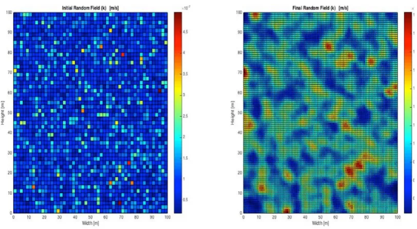
(17) 17. 3. RDD simulation of partially immersed levees & element analysis Results from a RDD simulation of a partially immersed levee are presented in this chapter. Subsequently a part of the levee that is under the effect of the rapid drawdown is singled out for the element level elastic-plastic analysis. The immersed (upstream) part is subjected to RDD whereby the water acting as the overburden pressure propping the inward levee slope is lowered. Computer resource limitation prohibits large scale shear bands simulations of this type and are, as yet, unattainable by other researchers in the field [3], [4]. In elasticplastic coupled FE formulations when failure conditions are reached, the intense shearing results in very steep strain gradients requiring very small load and time increments in numerical procedures. This and elements refinement in these regions increase the computational and memory storage time requirements by a power law. To render this problem to a manageable size we opted to focus on studying the elastic version of the fullsize RDD problem. With the computationally attainable elastic material model we can simulate heterogeneity of the material through randomness to reveal the state of the levee in regions with ensuing high shear and water pressures. In the following part we will look at the shear-region problem on an element scale. The small scale problem is computationally attainable on a personal computer to handle shear bands in heterogeneous elastic-plastic and coupled FE simulations. The RFEM is used to analyze the small and large scale problems. 3.1 Random permeability field simulator. A random generated permeability field 𝑘 that represents soil heterogeneity is introduced in both the large and small scale simulations. Depending on the time scale, a lower permeability results in regions where water flow inside the pores of the soil is slower then in regions with higher permeability. Randomness is modelled in combination with the FEM to achieve a RFEM to represent the phenomenon of heterogeneity in the soil. The random field is generated using the local average subdivision method (LAS) [19], [23]. The algorithm first generates a standard normal distribution field based on a spatial correlation parameter 𝜃e . The random permeability field is then generated by the formula: 𝑘² = 𝑒. ³´µ (¶) ˆ·´µ (¸) ¹º. (35). Where 𝑘² is the permeability of the element with index i and 𝜇hi (») is the mean of the logarithm of 𝑘 described by the formula: 𝜇hi (e) = ln 𝜇e −. 1 𝜎 2 hi e. 3. (36). Where 𝜇e is the mean of the permeability 𝑘 and 𝜎hi e is the standard deviation of the logarithmic of 𝑘 described by the formula: 𝜎hi e. 3. = ln 1 +. 𝜎e 𝜇e. 3. (37).

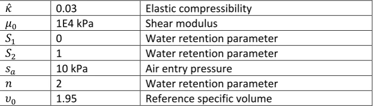
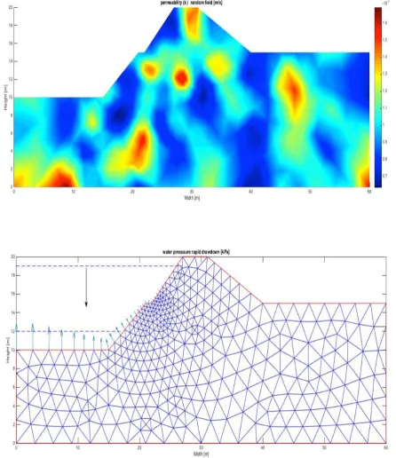
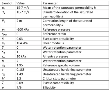
(18) 18 Where 𝜎e is the standard deviation of the permeability 𝑘. Finally 𝐺² is generated by the standard normal distribution field for the element with index i. The random permeability field is thus generated based on the parameters: 𝜇e , 𝜎e and 𝜃e . The LAS algorithm then subdivides the quadrilateral in smaller parts and subdividing the calculated permeability. This process is then repeated until a sufficiently smooth resolution is obtained in comparison to the element size of the FE problem. In the final step the random permeability field is projected on the finite element mesh. The result of a random LAS simulator is shown in Fig. 1 for 𝜇e = 1𝐸 t¾ 𝑚/𝑠, 𝜎e = 1𝐸 t¾ 𝑚/𝑠 , 𝜃e = 5 𝑚.. Figure 1 LAS algorithm: (a) initial random mesh; (b) refined random mesh. 3.2 Large scale RDD simulation. The RDD simulation consisting of a random permeability field, a FEM mesh of the levee slope as well as BC imposed on parts of the levee to model rapid drawdown, is schematized in Fig. 2a and b. The FE mesh consists of a mixed three noded triangular mesh with displacement and porewater pressure degrees of freedom. The soil consists of a hyperelastic clay layer with parameters summarized in table 1. The random permeability field is characterized by a the parameters with 𝜇e , 𝜎e and 𝜃e . The parameters are chosen to represent a typical Dutch stiff-clay levee in the northern part of the Netherlands. Symbol 𝜇e 𝜎e. Value 1E-7 m/s 1E-7 m/s. 𝜃e. 2m. 𝑝[ 𝜀T,[. -100 kPa 0. Parameter Mean of the saturated permeability 𝑘 Standard deviation of the saturated permeability 𝑘 Correlation length of the saturated permeability 𝑘 Reference pressure Reference strain.

(19) 19 𝜅 𝜇[ 𝑆2 𝑆3 𝑠5 𝑛 𝜐[. 0.03 1E4 kPa 0 1 10 kPa 2 1.95. Elastic compressibility Shear modulus Water retention parameter Water retention parameter Air entry pressure Water retention parameter Reference specific volume. Table 1: soil parameters. Before RDD takes place the levee slope is first compressed by a water level of 19 m against a levee slope of 20 m. During this initial extended (drained) time period the levee is saturated and in a compression state with steady state in-situ water pressures and effective stresses (𝝈) in equilibrium with the fixed porewater pressure BC of the state prior to RDD. This is followed by specifying BC which prescribe the removal of horizontal and vertical degrees of freedom on the bottom of the mesh and the removal of horizontal degrees of freedom on the left and right side of the mesh. This mesh represents a levee slope that is placed on a rigid soil layer. When the porewater pressure 𝑝, on a boundary node adjacent to air exceeds atmospheric pressure (𝑝5 ), a BC is created that is the result of seepage of water from the pores of the soil. This represents the phreatic water head in the body of the levee prior to RDD. This procedure is similar to that used in [19], [23]. After the initial phase, the RDD condition is introduced by lowering the water level in a period of 10 hours. The RDD is reflected in the BC through the pressure- and fixed porewater pressure BC. The previous pressure BC of 19 meter is removed and replaced with a pressure BC that is the result of a water level of 2 meter. The pressure gradient in Fig. 2b shows the magnitude and direction of the resulting pressure gradient. The previous fixed porewater pressure BC is also replaced with a porewater pressure BC that is the result of a water level of 2 meters. The final adjustment replaces the previous porewater pressure BC with a seepage BC. In doing so porewater can flow from out of the elements that where previously adjacent to water..

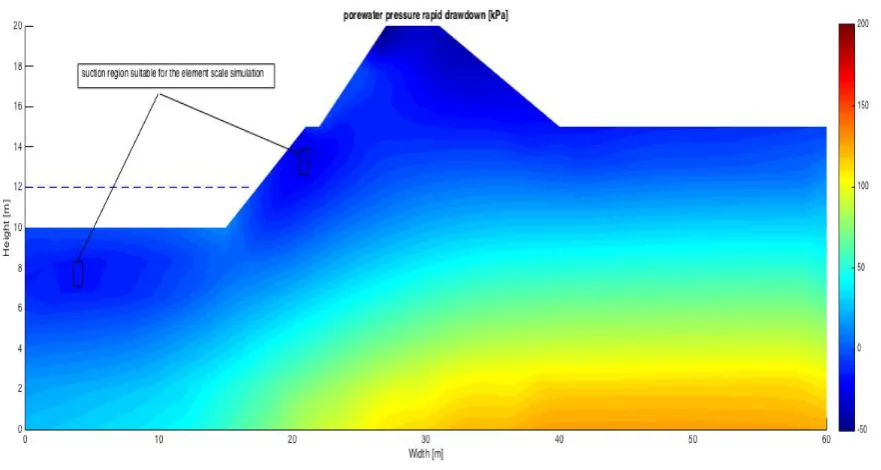
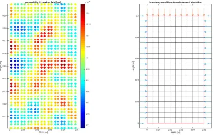
(20) 20. Figure 2: FEM mesh element scale simulation: (a) random permeability field; (b) mesh and BC. Because the time period choses in relatively short, the in-situ excess porewater pressure as well as air remains entrapped in the levee slope. This results in unsaturated regions inside the levee when porewater pressure becomes negative since the levee is depressurized during RDD to such an extent that trapped air bubbles expand and thus result in suction (𝑐9 ) according to equation (3). The effects of the BC on porewater pressure inside the slope after compression and subsequent decompression during RDD is displayed in Fig. 3a and b..

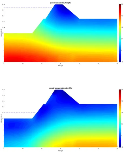
(21) 21. Figure 3 Development of porewater pressure: (a) initial phase; (b) RDD phase. The unsaturated coupled elastic results are produced by solving the global equations (1) to (11) of chapter 2 with the algorithm described in Box 1. Since plasticity was omitted when forming the local equations, the effect of plastic yielding is not observed anywhere and is not part of the solution as the global solution involves an elastic stiffness matrix assembled from the local elements..

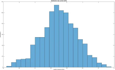
(22) 22 Figure 3 highlights that RDD decompresses the levee slope allowing trapped air bubbles (voids) to form unsaturated regions in the levee slope on both sides. In these regions the degree of saturation (𝑆( ) is less than 100% and thus permeability is reduced due to the induced air voids [10]. This is typically observed within the region of flow reversal between the compression and decompression states on the inward slope side. These results prove, among other things, the onset of heterogeneity associated with the flow and saturation reversal phase and their governing parameters from RDD at the large (levee), mezzo (void) and macro (element/small and local) scale. Flow reversal is shown in the above Fig. 3b. In other regions of the large scale problem, like the core of the levee, porewater pressures remain constant in the time period just after RDD since the drainage path is longer there, where seepage has not yet had time to reduce the overall porewater pressure. On longer time scales the unsaturated regions in this levee might saturate again due to seepage that is a result of the water pressure gradient inside- and water levels outside the levee slope. In this transient period, the weight of the levee, the water-pressure gradient and suction will affect the onset of shear bands. As mentioned earlier, due to computational constraints this is not simulated directly. In Fig. 4 the regions of interest are displayed where possibly shear bands could form in the unsaturated part of the levee under RDD.. Figure 4 RDD: suction regions of interest for element scale simulation. To study the influence of heterogeneity on the magnitude of suction a Monte Carlo analysis is repeating the RDD iterations where for each instance a random field is generated based on the statistical parameters characterizing the permeability distribution (𝜇e , 𝜎e , 𝜃e ). Any distribution could be used but in this study we specified the standard log-normal.

(23) 23 distribution. The results are displayed in Fig. 5. For each Monte Carlo simulation, the maximum suction after RDD was calculated and stored for each iteration.. Figure 5: histogram with the distribution of suction after 1000 RDD Monte Carlo simulations. The results of figure 5 prove that the random permeability field influences the magnitude of suction pressure in the unsaturated regions resulting from RDD. It is likely that other parameters in table 1 also influence the magnitude of suction. However, this is outside the scope of this research. It can be concluded that RDD results in an unsaturated region for a limited transient time period inducing sudden critical and rather peculiar conditions: inward undrained shear instability, directional seepage reversal, induced inhomogeneity and anisotropy of mechanical and other key parameters governing flow and deformations such as saturation and permeability [5], [6], [15]. This is a complex multi-variate system of a three-phase material in which failure is no longer governed by the original, steady state parameters alone but rather dominated by the formation of randomly distributed heterogeneity possibly inducing irregular shear bands and instability during or shortly after the RDD. To further study this a region is singled out in the locality shown in Fig. 4 and a small scale element level simulation is performed with the full elastic-plastic coupled equations (1) to (33) to study the onset of shear bands during conditions similar to RDD. The scale factor of the two simulations is 1000:1..

(24) 24 3.3 Shear band simulation. The small-scale simulation consists of a similar random permeability field as generated for the RDD large-scale simulation that is adjusted for the scale of the simulation. The scale of the spatial correlation length 𝜃e is therefore adjusted by a factor 1000. This is necessary since the correlation length is limited to the element size. To generate a meaningful random permeability field 𝜃e needs to be adjusted to the new element scale. The standard deviation is not adjusted to compensate for the size of the problem. This is because the exact variation to correlation length scale is practice is not known. The current practice in the Netherlands dictate that clay layers regardless of size can vary in permeability anywhere within the range of 1E-6 m/s and 1E-8 m/s [8]. The FEM mesh consists of mixed four node quadrilateral elements with displacement 𝒖 and porewater pressure 𝑝, degrees of freedom. The soil consists of a hyper- elasticplastic cohesive (clayey) material as given by the elastic-plastic model in chapter 2. The parameters are summarized in table 2. Symbol 𝜇e 𝜎e. Value 1E-7 m/s 1E-7 m/s. 𝜃e. 2m. 𝑝[ 𝜀T,[ 𝜅 𝜇[ 𝑆2 𝑆3 𝑠5 𝑛 𝜐[ 𝑐2 𝑐3 𝑀 𝜆 𝜌. -100 kPa 0 0.03 1E4 kPa 0 1 10 kPa 2 1.95 0.185 1.49 1.2 0.09 7/9. Parameter Mean of the saturated permeability 𝑘 Standard deviation of the saturated permeability 𝑘 Correlation length of the saturated permeability 𝑘 Reference pressure Reference strain Elastic compressibility Shear modulus Water retention parameter Water retention parameter Air entry pressure Water retention parameter Reference specific volume Unsaturated hardening parameter Unsaturated hardening parameter Critical state parameter Plastic compressibility Ellipticity. Table 2: soil parameters. The same elastic and stochastic mean parameter is used as as in the case of the stiff clay levee. The plasticity parameters represent a stiff normally consolidated clay similar to [1] and is likely to represent a clay levee in the northern part of the Netherlands. The plain-strain sample is subjected to pressure BC that result in an isotropic confining pressure of 100 kPa. On the top and bottom of the FEM mesh the degree of freedom for vertical displacement is removed. One bottom corner node has both horizontal and vertical.

(25) 25 degrees of freedom removed for stability. The shear band is generated by moving the top boundary vertically during the simulation in a displacement-controlled time period of 350 seconds. The FEM mesh and BC are displayed in Fig. 6a en b. The initial condition consists of an isotropic (positive) compressive stress of 100 kPa 𝑝[ and a (negative) suction pressure of 10 kPa. A shear band that is generated by the model is then strictly the result of the random permeability field. Note that in reality many other random fields of parameters could result in shear bands. During the compression the soil element is locally undrained since in the relative short time period of 350 seconds no seepage over the boundary of the element can take place although seepage still takes place inside the soil sample elements.. Figure 6 FEM mesh element scale simulation: (a) random permeability field; (b) mesh and BC. 3.4 Shear bands results with the RFEM. The effect of the random permeability field under the compression condition is in analogue to a discontinuous field problem. Elements with lower permeability in the simulation are not as well connected to each other nor to the elements with a high permeability as in a uniformly distributed permeability in a continuous field. The implication of this is that porewater in low permeability elements tends to stick around in the element unable to escape increasing porewater pressure instead. In such situations low permeability regions tend to be dominant. When a soil layer or sample is modelled using a single value for permeability, the overall behavior of all the soil elements is influenced. When a random permeability field is specified however mainly elements that are well connected distribute the pore pressures between them very fast. When a well-connected element borders on a not as well connected one, porewater is confined increasing pore pressure in those well connected regions. This effect is further influenced by air inside the pores. Air in the voids further decreases permeability and thus regions with a lower degree of saturation in the soil.

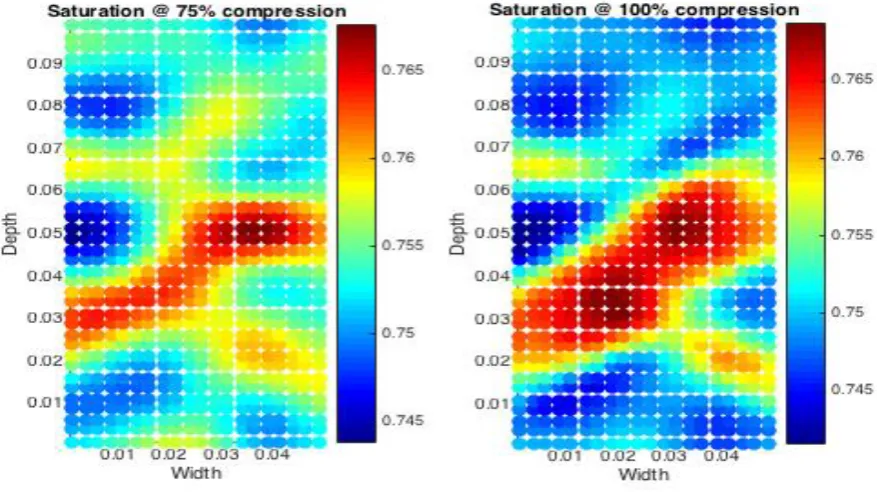
(26) 26 element tend to remain unsaturated longer during the compression then regions with a higher degree of saturation [15]. This is illustrated in Fig. 7a-d which shows stages in the development of the degree of saturation during compression. Notice that the legend of all graphs in this section are scaled (non-dimensional) values with respect to the magnitude of the degree of saturation. During the compression phase the increase in saturation for most elements of the FE simulation of the soil sample remains largely constant. However, the degree of saturation of the element with a higher permeability tend to increase faster creating disparity of the degree of saturation within the soil sample..

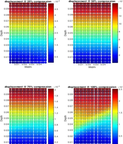
(27) 27. Figure 7 degree of saturation: (a) 25 % compression; (b) 50% compression; (c) 75% compression; (d) 100% compression. When comparing the results in Fig. 7 and 8 the initial disparity in degree of saturation that is the result of the random permeability field influences porewater pressure and displacement increase. This in turn influences de degree of saturation further affecting displacement and porewater pressure [10]. This process cascades to a points that displacement, porewater pressure and thus degree of saturation localizes to an area inside the soil. The initial random permeability field therefore creates a runaway condition where the underlying coupled mechanism enhanced itself to the point of a clearly defined region where the degree of saturation is substantial different similar to [1]. A typical feature of solving the coupled Biot equations is that porewater pressure is coupled to soil deformation. When a pressure BC changes, for example from an external load, it changes total stress in the soil which is taken at first by the water in the pores. Depending on permeability and the size of the time-step (Δt) this increases in porewater pressure is transformed with time to effective inter-particle soil stresses and deformation of the pores. When a random permeability field is created in the soil element under compression, effective stresses, deformation and porewater pressure are affected directly. As was explained in the previous part the randomness itself also influences porewater pressure. It can therefore be concluded that the random permeability field, depending on 𝜇e , 𝜎e and 𝜃e will create a first order effect in the disparity in porewater pressure and thus effective stresses and deformation under compression conditions. This is further illustrated in Fig. 8ad with the magnitude and the gradient of the deformations 𝐮 . Notice that the degree of saturation of 6d closely mirrors the extreme deformation gradient in 7d. This is a shear band that is further discussed in the next paragraph..

(28) 28. Figure 8 deformation (gradient): (a) 25 % compression; (b) 50% compression; (c) 75% compression; (d) 100% compression. Since the random permeability field creates a first order effect through the disparity of porewater pressure it also create a second order effect in the degree of saturation, as confirmed similarly in reference [1]. The degree of saturation in turn affects permeability as trapped air will deter seepage through the air-filled pores of the soil. In the unsaturated.

(29) 29 regions of the element, the degree of saturation in turn influences inter-particle friction and therefore elastic-plastic deformation behavior. The increase of degree of saturation will therefore decrease the effective pre-consolidation pressure (𝑝R ) causing the soil deformation to become plastic [2]. This third order dependency on the random permeability field in which a soil behaves elastically while others yield plastically will cause the yielding part to deform irreversible. The area’s that irreversible deform further affect porewater pressure inside high permeability regions adding to the cascading process and result in the onset of a shear band in these regions. In fact, through this process the location and moment when shear bands emerge is greatly dependent on the random permeability field as compression will further shear and compress regions with a high degree of saturation. This is illustrated in Fig. 9a-d where deformation is expressed in terms of sum of the x-, yand z- component of the engineering strain tensor 𝜺𝒆 . This is the so-called volumetric strain invariant similar to equation (16). Notice that the region of compressive deformation closely resembles the increase in the degree of saturation. Some oscillations in the strain field was also observed that will be further discussed at the end of this chapter..

(30) 30. Figure 9 volumetric strain invariant: (a) 25 % compression; (b) 50% compression; (c) 75% compression; (d) 100% compression. However, it is equally possible, depending on the random permeability field first, second and third order effects, that a stress point is actually on the dilative side of the yield surface [2]. In the elastic region described earlier the soil elements can sustain larger deviatoric stresses 𝑞 causing the stress point to move to the dilative side. This is illustrated in Fig. 10 by the development of the stress ratio. The higher permeability regions with high values of compressive volumetric strain of Fig. 8 will display compressive behavior while the lower permeability will instead move to the dilative side of the yield surface causing stress ratios exceeding the critical state. However, since the stress point is now on the dilative side, softening will occur causing the formation of sustained shear bands in the regions where the compressive behavior is near dilating regions. This is illustrated in Fig. 11 by the deviatoric strain invariant that shows the development of a shear band near the regions in the soil elements where dilating- and compressing regions are near each other. Because a shear band emerges, the confining pressure will eventually be insufficient to contain the soil sample during the compression phase. The resulting decompression reaction will cause the soil sample to finally collapse along the shear bands described in Fig. 7 to 10 of the initial compression phase in the large-scale RDD levee case simulated in this chapter..

(31) 31. Figure 10 stress ratio –q/p: (a) 25 % compression; (b) 50% compression; (c) 75% compression; (d) 100% compression.

(32) 32. Figure 11 deviatoric strain invariant: (a) 25 % compression; (b) 50% compression; (c) 75% compression; (d) 100% compression. It was found that both compressive and dilative shear bands closely resemble RDD conditions in the real large-scale situation, where instability caused by sudden intense shearing in unsaturated plastic yielding regions is mainly the result of porewater pressure.

(33) 33 increase. In the case of RDD this porewater pressure increase in the unsaturated region of the levee slope could be the result of seepage between the pressure gradient after RDD. The sudden decrease in porewater pressure causing a decrease in the degree of saturation directly after RDD actually increases the chance of levee failure since unsaturated behavior increases the magnitude of softening that causes shear bands. The levee slope will therefore behave more brittle in unsaturated rapid drawdown conditions causing sudden collapse [13]. More research is needed to confirm these results for the large scale RDD problem. Also more research is needed to correlate the random permeability field parameters 𝜇e , 𝜎e and 𝜃e with the first, second and third order effects and whether compressive or dilative shear bands will emerge. Each random permeability field results in a different shear band as was shown by simulations performed using different random permeability fields (see appendix A). 3.5 numerical difficulties. Quadrilateral element, although in general more stable, portray a very stiff reaction with regards to volumetric strain and thus to the effective volumetric pressure field (𝑝′). This does result in volumetric strain and stress oscillations as can be observed in Fig. 9 and 10 on the edges of the shear band. This is not a physical effect since different type of element like triangles mitigate this problem. Triangle are however prone to element direction bias. It was found that quadrilateral elements as used here are unable to properly simulate regions of the soil element where an incompressible condition is present. This incompressible condition is the result of the soil compressing to a point where the critical state is reached. From that point on the soil will not undergo any further stress changes during compression under continues strain [20]. Due to this incompressible condition the confining pressure of the soil samples is insufficient resulting in the decompressing condition mentioned earlier. This can me observed in Fig 11. Where shear strain is due to decompression actually decreasing between 75% compression and 100% compression. The simulation is thus working consistent with qualitative physical understanding however due to the limitations of continuous displacement and porewater pressure field used here somewhere after 50% compression the simulation fails to capture the true physical situation. In a physical situation the soil sample would crack when the confining pressure is insufficient. The incompressible condition in that case would spur this process. However, the discontinuous displacement and porewater pressure mesh that is necessary for this kind of simulations is outside the scope of this research [11]. Another volumetric numerical difficulty is related to porewater pressure. Aside from parts of a soil sample reaching the critical state, the incompressible condition is also reached by the combination of a very low permeability and time-step. As was mentioned earlier, when deformation inside a shear band increases the gradient of the displacement also increases..

(34) 34 This in turn causes nonlinear elastic-plastic behavior resulting in smaller time-steps. In a coupled system, this will also lead to porewater pressure oscillations as the time step is gradually decreased when deformation is increased [22]. This results in almost zero water flow while deformation is increasing and thus the soil will behave incompressible as water itself cannot compress under normal conditions but only diffuse through the pores. A straightforward method to resolve this problem is the ppp algorithm where the equal order displacement and porewater pressure field is enhanced by a spatial and temporal porewater pressure field [21]..

(35) 35. 4 Concluding remarks 4.1 conclusion. It can be concluded that the introduction of random k-field in the RFEM algorithm developed during this study has provided for the first time a rational simulation of RDD of levees meriting further research to efficiently depict real field problems. The field problem was simulated with a Monte Carlo simulation that proved that with elastic material description the random permeability field influences the magnitude of porewater pressure and suction in the levee slope. This in turn influences flow reversal during rapid drawdown, deformation and effective stresses. A subsequent element level analysis with a random kfield that used BC, state parameters and initial conditions of the large scale analysis to simulate RDD resulted in the formation of localized shear bands. This localization is the result of soil behavior that on several levels interact with the random permeability field through porewater pressure and suction. In turn influencing the degree of saturation that further influences permeability, elastic-plastic yielding and effective stresses in the soil. This will finally result in either dilative or compressive elastic-plastic deformation behavior. The onset of subsequent shear bands through the random k-field might in reality be the cause for levee collapse during RDD. Other parameters apart from permeability might have similar affects on the formation of shear bands. Furthermore, different rapid drawdown scenario’s, soil types and levee geometry might influence the onset of shear bands and the type of random fields that influences it. This research also merits the use of advanced soil models that capture unsaturated soil behavior in an RFEM context to simulate RDD. The complicated irrecoverable elastic-plastic soil behavior is a major driver for the location, magnitude and type of shear band that is the result of RDD. The saturated, drained, limit-state models that are used in current Dutch practice will disregard this soil behavior possible leading to erroneous results. However, the use of RFEM in combination with unsaturated models on a scale that simulate shear bands is at this time not an option due to compounding computing costs. 4.2 further research. Further research is needed to cross examine all the variations of soil types, RDD scenario’s and levee geometry to single out variations that cause levee collapse. Furthermore, the influence of other random parameters other then permeability need to be investigated to ascertain which parameters are relevant during rapid drawdown. It is also important to note that although RDD is the levee failure mechanism that is studied in this research, further research should be undertaken on how random fields influence other types of levee failure during flooding periods. These results should then be compared to saturated, drained, limitstate results of current Dutch practice to ascertain the need to incorporate more complicated soil models and random fields. A major obstacle in this is the fact that it is difficult to simulate shear bands in large scale problems especially whit regards to complicate unsaturated soil models. Further research is needed to improve performance of these type of simulations while still able to capture the type of failures that where simulated.

(36) 36 in this research. It is therefore recommended to develop a linear-elastic model that incorporates (unsaturated) hardening. To enhance knowledge of random fields laboratory testing should also be included since the numerical observation have to match the practical observations. The correlation length, mean and standard deviation of permeability can for example be observed through porosity of the soil with a Magnetic Resonance Imaging (MRI). The sample can then be sheared to failure in a triaxial-test in order to obtain the shear strength of the sample with the permeability distribution. Subsequent FE analysis should obtain similar results that deviate from a Fe analysis with a soil layer with constant permeability. This is only one example of several possibilities where laboratory testing could improve the knowledge of actual random fields in practice..

(37) 37. Reference [1] Borja, R. I., et al. (2013). "Critical state plasticity. Part VII: Triggering a shear band in variably saturated porous media." Computer Methods in Applied Mechanics and Engineering 261: 66-82. [2] Alonso, E. E., et al. (1990). "A Constitutive Model for Partially Saturated Soils." Geotechnique 40(3): 405-430. [3] Borja R.I. et al., (2012) Multiphysics hillslope processes triggering landslides, Acta Geotech. 7, 261–269. [4] Borja R.I. et al., (2012) Factor of safety in a partially saturated slope inferred from hydromechanical continuum modeling, Int. J. Numer. [5] Griffiths, D. V. et al., (1999). "Slope stability analysis by finite elements." Geotechnique 49(3): 387-403. [6] Pinyol N.M., et al., (2008). "Rapid Drawdown in slopes and embankments." Water Resources Research 44. [7] Pater W.H., Retentiegebieden Hunze en Aa’s, gebruik en mitigatie negative bijeffecten, 2010 [8] Termaat R.J. et al., Construeren met grond, Civieltechnisch Centrum Uitvoering Research en Regelgeving, 1992 [9] Lambe T.W. et al., Soil Mechanics, John Wiley & Sons, 1969. [10] Van Genuchten M.Th., (1980), A closed-form equation for predicting the hydraulic conductivity of unsaturated soils, Soil Sci. Soc. Am. J. 44 892–898. [11] Callari C., et al., (2010), Strong discontinuities in partially saturated poroplastic solids, Comput. Meth. Appl. Mech. Engrg. 199, 1513–1535. [12] Meschke G., et al., (2003), Numerical modeling of coupled hygromechanical degradation of cementitious materials, J. Engrg. Mech. 129, 383–392. [13] Borja, R. I. (2004). "Cam-Clay plasticity. Part V: A mathematical framework for threephase deformation and strain localization analyses of partially saturated porous media." Computer Methods in Applied Mechanics and Engineering 193(48-51): 5301-5338. [14] Borja R.I. et al., (1998), Cam-Clay plasticity Part III: extension of the infinitesimal model to include finite strains, Comput. Meth. Appl. Mech. Engrg. 155 , 73–95..

(38) 38 [15] Fredlund D.G et al., Unsaturated Soil Mechanics in Engineering Practise, John Wiley & Sons, 2012. [16] Gudehus G., (1973) , Elastoplastische Stoffgleichungen für trockenen Sand, IngenieurArchiv 42 151–169. [17] Chen W.F., et al.,Plasticity for Structural Engineers, Springer Verlag, Berlin, Germany, 1988. [18] Borja R.I., et al., (1997), Coupling Plasticity and Energy-Conserving Elasticity Models for Clay, Journal of Geotechnical and Geotechnical Engineering, 123(10): 948-957 [19] Fenton et al., (2008). Risk Assesment in Geotechnical Engineering. New Jersey, John Wiley & Son's. [20] Schofield A., et al., Critical State Soil Mechanics, McGraw-Hill, 1968 [21] White J.A., et al., (2008). "Stabilized low-order finite elements for coupled soliddeformation/fluid-diffusion and their application to fault region transients." Computational Methods Applied Mechanical Engineering (197): 4353-4366. [22] Smith I.M., et al., (2014). Programming the Finite Element Method. New Jersey, John Wiley & Son's. [23] Griffiths, D. V. et al., (1990). "On the Variable Mesh Finite-Elements Analysis of Unconfined Seepage Problems ." Geotechnique 40(3): 523-523. [24] Gallipoli, D., et al. (2003). "An elasto-plastic model for unsaturated soil incorporating the effects of suction and degree of saturation on mechanical behaviour (vol 53, pg 123, 2003)." Geotechnique 53(9): 844-844..

(39) 39. Appendix A: additional results for a different random permeability field. nd. Figure 12 degree of saturation 2 field: (a) 25 % compression; (b) 50% compression; (c) 75% compression; (d) 100% compression.

(40) 40. nd. Figure 13 deformation (gradient) 2 field: (a) 25 % compression; (b) 50% compression; (c) 75% compression; (d) 100% compression.

(41) 41. nd. Figure 14 volumetric strain invariant 2 field: (a) 25 % compression; (b) 50% compression; (c) 75% compression; (d) 100% compression.

(42) 42. nd. Figure 15 stress ratio –q/p 2 field: (a) 25 % compression; (b) 50% compression; (c) 75% compression; (d) 100% compression.

(43) 43. nd. Figure 16 deviatoric strain invariant 2 field: (a) 25 % compression; (b) 50% compression; (c) 75% compression; (d) 100% compression.

(44) 44. Appendix B: derivatives for Newton solver global and local equations Step 5 of box 1 describes a Newton algorithm that is needed to iterative solve the global system of equations. Chapter 2 describes the coupled equations themselves. For a Newton iteration the derivatives of these equations are also necessary. The derivative of the global 𝒅𝑹 equations is describes as where R is the vector with the global equations and U is the 𝒅𝑼. solutions for displacement and porewater pressure at each node of the FE mesh. Thus represent the derivative of the global equations with respect to displacement and porewater pressure:. 𝒅𝑹. =. 𝒅𝑼. 𝑨𝟏 𝐀𝟐 𝑨𝟑 𝑨𝟒. 𝒅𝑹 𝒅𝑼. (34). with: m3. 𝛁 𝒔 𝑵𝑻 𝑪 𝛁 𝒔 𝑵𝑑𝐴. 𝑨𝟏 =. (35). m2 m3. 𝛁 𝒔 𝑵𝑻 𝑨 − 𝑆𝑟𝟏. 𝑵𝑑𝐴. 𝑨𝟐 = −. (36). m2 m3. 𝑵𝒕 𝑆( 𝟏. 𝛁 𝒔 𝑵𝑑𝐴. 𝑨𝟑 =. (37). m2 m3. 𝑨𝟒 = m2. 𝑑𝑆( 𝑵𝒕 𝟏. 𝛁 𝒔 𝑵𝑑𝐴 + 𝑑𝑝, m3. 𝑬𝒕. −∆𝑡 m2. m3. 𝑵𝒕 1 − ∅; m2. 𝑑𝒗 𝑑𝐴 𝑑𝑝,. 𝑑𝑆( 𝑵𝑑𝐴 … 𝑑𝑝,. (38). where 𝑪 is either the elastic constitutive stress-strain tensor or the elastic-plastic constitutive stress-strain tensor dependent on the yielding of the material. 𝑨 is the stresscapillary tensor that quantifies the influence of capillary porewater pressure or suction on the effective inter-particle stresses of the material. 𝑆𝑟 stands for: 𝑆𝑟 = with:. 𝑑𝑆( 𝑝 + 𝑆( 𝑑𝑝, ,. (39).

(45) 45 𝑑𝑆( = m 𝑆3 − 𝑆2 𝑑𝑝,. 𝑐9 𝑠5. 1+. * t uˆ2. 𝑛. 𝑐9 𝑠5. *t2. 1 𝑠5. (40). with: 𝑑𝒗 𝑘 = −𝑘? ∗ ; 0 𝑑𝑝,. where. …eÈ …9É. 𝑑𝑘? 𝑘; 0 𝑬– ∗ 𝑘; 0 𝑑𝑝,. 𝑝, 0 𝑬 +𝑧 𝑵 𝑘; 𝜌, 𝑔. 41. is calculated with the finite (central) difference method for practical reasons.. The algorithm for this is: 𝑑𝑘? 𝑘? 9Ê?; − 𝑘? u²* =− 𝑑𝑝, ℎ. (42). where: 𝑘?. 9Ê?;. =. 2 𝜃3. 1− 1−. and: 𝜃=. 𝑆( − 𝑆2 𝑆3 − 𝑆2. 2 u 3 u 𝜃. (44). with: 𝑆( = 𝑆2 + 𝑆3 − 𝑆2. (43). 1 𝑐9 + ∗ ℎ 2 1+ 𝑠5. *. tu. (45). 2. where h is a small quantity. This is similar for 𝑘? u²* where 𝑐9 − ∗ ℎ is used instead. 3. Step 4 of box 2 describes a Newton algorithm that is needed to iterative solve the local system of equations. Chapter 2 describes the local equations themselves. The derivative of 𝒅𝒓 the local equation is where r stands for the local equation vector and x for the local 𝒅𝒙 solution vector consisting of the strain tensor 𝜺𝒆 and plastic multiplier Δ𝜆. 𝒅𝒓 𝒂𝟏 𝒂𝟐 = 𝒂 𝒂 𝟑 𝟒 𝒅𝒙 where. (46).

(46) 46 𝜕3𝑮 𝜕 𝟐 𝑮 𝜕𝑝R 𝒂𝟏 = 𝑰 + Δ𝜆 𝑪+ 𝜕𝝈𝟐 𝜕𝝈𝑝R 𝜕𝜺𝒆. 𝒂𝟐 =. 𝜕𝑮 𝒂𝟑 = 𝜕𝝈. 𝜕𝑮 𝜕𝝈. £. (47). (48). 𝑪+. 𝜕𝑭 𝜕𝑝R 𝜕𝑝R 𝜕𝜺𝒆. 𝒂𝟒 = 0. (50). (49). r• 𝑮. r𝑮. where 𝑪 is the elastic constitutive stress-strain tensor. The derivative tensor and r𝝈 r𝝈𝟐 are the first and second derivative from the flow surface that in the case of associative plasticity is the same as the yield surface (14). The derivate are derived with the first and second order (central) finite difference method similar to (42). And: 1 3 1 3 𝜕𝟐𝑮 = 1 𝜕𝝈𝑝R 3 0 0 0. (51). 𝜕𝑭 = −𝑝Î 𝜕𝑝R. (52). and:. and:. 𝜕𝑝R = 𝑏 𝑒5 𝜕𝜺𝒆. −𝑝R,*. 𝜀TV − 𝜀TU( 𝜆−𝜅. œt2. 𝑝R,*. 𝜀TV − 𝜀TU( 𝜆−𝜅. 1 1 1 1 𝜆−𝜅 0 0 0. (53).

(47) 47. Appendix C: using the Matlab program (element simulation) The Matlab program for the element simulation utilizes a random permeability field that can be adjusted to facilitate different random or uniform distribution. For the sake of brevity, no other parameters or boundary conditions can be adjusted. There is also an option to utilize a Monte-Carlo analysis when by simulations a value is chosen larger then unity. The user can adjust the following parameters: 𝜇e = mean permeability. Usually chosen in the range of 1E-6 to 1E-7. 𝜎e 3 = standard deviation. Usually chosen in the range 1:100 from the mean permeability 𝜃e = correlation length. Usually chosen between 0 and ∞ simulations = usually chosen between 1 and 1E4 When correlation length is chosen equal to 0 no correlation length is specified and a random normal distribution is generated in the size of one element. When correlation length is chosen equal to infinite a homogenous permeability is generated for the element equal to the mean permeability. When simulation 1 is chosen detail graphs will be generated that display displacement, stresses, strain, pre-consolidation pressure, porewater pressures, stress ratio’s etc. When simulation is chosen larger then 1 a histogram will be displayed with the max shear stress and max hydraulic gradient..

(48)

No results found