6PRIG 2UGOTGS!2GRO]OFGZ
- @JGSKS ?UDNKTTGF HPR TJG 0GIRGG PH <J0
CT TJG
AOKVGRSKTY PH ?T" -OFRGWS
&$%%
2UMM NGTCFCTC HPR TJKS KTGN KS CVCKMCDMG KO
>GSGCREJ,?T-OFRGWS+2UMM@GXT
CT+
JTTQ+##RGSGCREJ!RGQPSKTPRY"ST!COFRGWS"CE"UL#
<MGCSG USG TJKS KFGOTKHKGR TP EKTG PR MKOL TP TJKS KTGN+
JTTQ+##JFM"JCOFMG"OGT#%$$&'#%)*(
@JKS KTGN KS QRPTGETGF DY PRKIKOCM EPQYRKIJT
Points to Static Equilibria
Jorge Fuentes-Fern´andez
Thesis submitted for the degree of Doctor of Philosophy
of the University of St Andrews
1. Candidate’s declarations:
I, Jorge Fuentes Fern´andez, hereby certify that this thesis, which is approximately 45 000 words in length, has been written by me, that it is the record of work carried out by me and that it has not been submitted in any previous
application for a higher degree.
I was admitted as a research student in October 2007 and as a candidate for the degree of Doctor of Philosophy
in October 2008; the higher study for which this is a record was carried out in the University of St Andrews between 2008 and 2010.
Date: Signature of Candidate: .
2. Supervisor’s declaration:
I hereby certify that the candidate has fulfilled the conditions of the Resolution and Regulations appropriate for the
degree of Doctor of Philosophy in the University of St Andrews and that the candidate is qualified to submit this thesis in application for that degree.
Date: Signature of Supervisor: .
3. Permission for electronic publication:
In submitting this thesis to the University of St Andrews we understand that we are giving permission for it to be
made available for use in accordance with the regulations of the University Library for the time being in force, subject to any copyright vested in the work not being affected thereby. We also understand that the title and the
abstract will be published, and that a copy of the work may be made and supplied to any bona fide library or research worker, that my thesis will be electronically accessible for personal or research use unless exempt by
award of an embargo as requested below, and that the library has the right to migrate my thesis into new electronic forms as required to ensure continued access to the thesis. We have obtained any third-party copyright permissions
that may be required in order to allow such access and migration, or have requested the appropriate embargo below.
The following is an agreed request by candidate and supervisor regarding the electronic publication of this
thesis:
Access to Printed copy and electronic publication of thesis through the University of St Andrews.
Date:
In magnetised plasmas, magnetic reconnection is the process of magnetic field merging and recombination through which considerable amounts of magnetic energy may be converted into other forms of energy. Reconnection is a
key mechanism for solar flares and coronal mass ejections in the solar atmosphere, it is believed to be an important source of heating of the solar corona, and it plays a major role in the acceleration of particles in the Earth’s
magnetotail. For reconnection to occur, the magnetic field must, in localised regions, be able to diffuse through the plasma. Ideal locations for diffusion to occur are electric current layers formed from rapidly changing magnetic
fields in short space scales. In this thesis we consider the formation and nature of these current layers in magnetised
plasmas.
The study of current sheets and current layers in two, and more recently, three dimensions, has been a key field of research in the last decades. However, many of these studies do not take plasma pressure effects into
consideration, and rather they consider models of current sheets where the magnetic forces sum to zero. More recently, others have started to consider models in which the plasma beta is non-zero, but they simply focus on the
actual equilibrium state involving a current layer and do not consider how such an equilibrium may be achieved
physically. In particular, they do not allow energy conversion between magnetic and internal energy of the plasma on their way to approaching the final equilibrium.
In this thesis, we aim to describe the formation of equilibrium states involving current layers at both two and three dimensional magnetic null points, which are specific locations where the magnetic field vanishes. The
dif-ferent equilibria are obtained through the non-resistive dynamical evolution of perturbed hydromagnetic systems. The dynamic evolution relaxes via viscous damping, resulting in viscous heating.
We have run a series of numerical experiments using LARE, a Lagrangian-remap code, that solves the full magnetohydrodynamic (MHD) equations with user controlled viscosity and resistivity. To allow strong current
accumulations to be created in a static equilibrium, we set the resistivity to be zero and hence simply reach our equilibria by solving the ideal MHD equations.
We first consider the relaxation of simple homogeneous straight magnetic fields embedded in a plasma, and determine the role of the coupling between magnetic and plasma forces, both analytically and numerically. Then,
we study the formation of current accumulations at 2D magnetic X-points and at 3D magnetic nulls with spine-aligned and fan-spine-aligned current. At both 2D X-points and 3D nulls with fan-spine-aligned current, the current density
becomes singular at the location of the null. It is impossible to precisely achieve an exact singularity, and instead, we find a gradual continuous increase of the peak current over time, and small, highly localised forces acting to
form the singularity. In the 2D case, we give a qualitative description of the field around the magnetic null using a singular function, which is found to vary within the different topological regions of the field. Also, the final
equilibrium depends exponentially on the initial plasma pressure. In the 3D spine-aligned experiments, in contrast, the current density is mainly accumulated along and about the spine, but not at the null. In this case, we find that
the plasma pressure does not play an important role in the final equilibrium.
Our results show that current sheet formation (and presumably reconnection) around magnetic nulls is held
back by non-zero plasma betas, although the value of the plasma pressure appears to be much less important for torsional reconnection. In future studies, we may consider a broader family of 3D nulls, comparing the results with
This work has been done under the umbrella of the SOLAIRE European training network, and was originally
designed as a collaboration between the E¨otv ¨os Lorand University of Budapest and the University of St Andrews. Although, circumstances have meant that it has become a project undertaken solely at the University of St Andrews,
within the Solar and Magnetospheric Theory Group. The work that has been carried for this thesis would not have
been possible without all the help and encouragement from,
My parents and sister, because it is thanks to them that I am who I am now, for encouraging me to choose my own
paths, and for giving me all their support in all the good and bad moments throughout my academic studies and my PhD.
My friends from Tenerife, and all the lecturers from the University of La Laguna, that led me to develop a keen interest in Astrophysics, and in solar and plasma physics, in particular.
All my friends in Budapest, for keeping me alive during one year of confusion and desperation, and all my friends in St Andrews for making it possible for me to build a life here in Scotland.
Nuri, for lots of things, because from the day I met her she has always been there for all my worries, and all my joys. And because by now, even though she is neither a physicist nor a mathematician, she knows more about the
structure of magnetic null points than many.
All the people from the Solar Theory Group in St Andrews, for understanding my situation when I first arrived at
the University, giving me all their help and support, and allowing me to finish my work with them, which was not originally stipulated.
Clare Parnell, for taking care of the full supervision of this work, for her neverending trust in me, and for giving me the opportunity to continue my academic career, here, in the University of St Andrews.
Alan Hood, for being a deep well of brilliant ideas, for his dedication, and for his ability to see the light when no one else could, and Dana Longcope, for a couple of interesting chats, and his ideas about X-points equilibria.
The SOLAIRE research network, for giving me this great opportunity, and for setting up an enormous number of international meetings and schools in which I have learnt much, met many interesting people and friends, and for
providing an alternative point of view to scientific research, based on the collaboration and interaction between different institutions, people and cultures.
Fernando Moreno-Insertis, coordinator of SOLAIRE, for his tremendous dedication and care for every single member of the network, and especially, for his empathy and extraordinary help, which made it possible for me to
finish my PhD in the University of St Andrews.
1 Introduction 1
1.1 A stairway to solar magnetohydrodynamics . . . 1
1.1.1 Nanautzin and the Sun . . . 1
1.1.2 About magnetism . . . 6
1.1.3 Ionised gases . . . 7
1.1.4 Describing the dynamics of conducting fluids . . . 9
1.2 The Equations of magnetohydrodynamics . . . 10
1.2.1 Maxwell’s equations and Ohm’s law . . . 11
1.2.2 Field lines and flux tubes . . . 12
1.2.3 Induction equation . . . 12
1.2.4 Fluids equations . . . 13
1.2.5 Restrictions and special terms . . . 15
1.2.6 Summary of MHD equations . . . 16
1.2.7 Energy considerations . . . 17
1.2.8 Magnetic forces . . . 18
1.3 MHD equilibria: Magnetohydrostatics . . . 19
1.3.1 MHS equilibria in 2D . . . 20
1.3.2 Classification of the MHS equilibria . . . 21
1.3.3 Models of MHS equilibria . . . 23
1.4 Magnetic null points . . . 25
1.4.1 Two-dimensional null points . . . 25
1.4.2 Three-dimensional null points . . . 27
1.5 Current sheets and reconnection . . . 33
1.5.1 Tangential discontinuities . . . 33
1.5.2 Current sheet formation . . . 33
1.5.3 Magnetic relaxation theory . . . 36
1.5.4 Magnetic reconnection . . . 37
1.6 Non-dimensional equations: Normalization . . . 39
1.7 Summary and main goals . . . 40
2.2.1 Viscous terms . . . 47
2.2.2 Shock viscosity . . . 47
2.3 The grid . . . 48
2.4 The Lagrangian step . . . 50
2.4.1 Predictor step . . . 51
2.4.2 Corrector step . . . 52
2.5 The remap step . . . 53
2.6 Resistive terms . . . 56
2.7 Stability condition . . . 56
2.8 Summary . . . 57
3 Relaxation of Parallel Magnetic Fields 59 3.1 Introduction . . . 59
3.2 Linear equations in 2D . . . 59
3.2.1 1D Perturbation across field lines . . . 62
3.2.2 1D perturbation along field lines . . . 65
3.2.3 2D perturbation . . . 66
3.2.4 Overview . . . 69
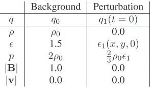
3.3 Numerical experiments: Setup . . . 69
3.3.1 Numerical specifications . . . 69
3.3.2 Initial conditions . . . 70
3.3.3 Perturbed total pressure . . . 72
3.4 Numerical experiments: Results . . . 72
3.4.1 Energetics . . . 73
3.4.2 Equilibrium . . . 75
3.4.3 Overview . . . 75
3.5 Importance of non-linear effects . . . 79
3.6 Parallel magnetic fields in 3D . . . 81
3.6.1 Linear equations . . . 81
3.6.2 Numerical experiments . . . 83
3.6.3 Overview . . . 84
4 Relaxation of 2D Magnetic Null Points 89 4.1 Introduction . . . 89
4.2 General properties . . . 90
4.2.1 Magnetohydrostatic equilibrium around an X-point . . . 90
4.2.2 Conservation of total current density . . . 90
4.3.2 Numerical studies in non-force-free fields . . . 93
4.3.3 Our approach to the problem . . . 93
4.4 Numerical experiments . . . 94
4.4.1 Numerical setup . . . 94
4.4.2 Energetics . . . 95
4.4.3 Final equilibrium . . . 96
4.4.4 Current density layer . . . 101
4.4.5 Singular current . . . 105
4.4.6 Overview . . . 105
4.5 Analytical description of the field . . . 107
4.5.1 Sample experiment . . . 107
4.5.2 Dependence with initial quantities . . . 110
4.5.3 Overview . . . 112
5 Relaxation of 3D Magnetic Null Points 113 5.1 Introduction . . . 113
5.2 Magnetic field configurations and numerical setup . . . 115
5.3 3D nulls with spine-aligned current . . . 116
5.3.1 Initial state . . . 116
5.3.2 Final equilibrium state . . . 118
5.3.3 Changes in current density and plasma pressure . . . 121
5.3.4 Overview . . . 121
5.4 3D nulls with fan-aligned current . . . 124
5.4.1 Initial state . . . 124
5.4.2 Final equilibrium state . . . 124
5.4.3 Current singularity . . . 128
5.4.4 Changes in current density and plasma pressure . . . 130
5.4.5 Overview . . . 132
6 Conclusions and Future Work 133 6.1 Discussion . . . 133
6.1.1 Results overview . . . 133
6.1.2 Implications for current sheet formation and magnetic reconnection . . . 135
6.1.3 General conclusions . . . 136
6.2 Future work . . . 136
Bibliography 138
Introduction
1.1
A stairway to solar magnetohydrodynamics
1.1.1
Nanautzin and the Sun
“Five worlds and five suns were created, one after the other. The first world was destroyed because its people acted wrongfully. They were eaten by ocelots and the sun destroyed. The second sun saw its people turned into
monkeys due to lack of wisdom. The third sun had its world destroyed by fire, earthquakes, and volcanoes because the people didn’t make sacrifices to the gods. The fourth world perished in a flood which also drowned its sun.
Before creating the fifth world, our world, the gods met in the darkness to see who would have the honor of igniting the fifth sun. Tecciztecatl volunteered. The gods built a big fire on top of a pyramid and the volunteer prepared to
throw himself into the flames. He was dressed in beautiful hummingbird feathers, with gold and turquoise. Four
times he tried to force himself into the suicidal fire but each time his fear drove him back. Then the lowliest of all the gods, Nanautzin, dressed in humble reeds, threw himself into the fire. Teccitztecatl was so ashamed that he too
jumped into the fire. The new sun rose into the sky giving light to the fifth world.” Credit: “Fifth World”, Toltec myth. WWU Planetarium.
Toltecs dominated the central part of Mexico from centuries X to XII. They are believed to be the predecessors of the Aztec culture, who thought of them as their wise ancestors. Most of the information that we now have about
the Toltecs comes embedded in their myths, in which, as many other civilizations from the past, they recognised the Sun as a powerful divinity, able to provide the Earth with heat and light.
Figure 1.1: Nanautzin in the flames. Nanautzin was known as the Scabby One, and was the ugliest and smallest of all gods, but with a modest courage, nonetheless. Credit: nativeweb.org.
What the Central American natives didn’t know is the true nature of what Nanautzin started by jumping into the sacred fire and therefore creating our Sun. He would have been, without doubt, a great alchemist, although his
humility would not have let him think about lead and gold, or at least, not before having had control over the most basic of the nuclear fusions: from single protons.
So, our humble Sun, being a relatively small young star, is powered continuously by nuclear fusion happening in its core, mainly combining two pairs of ionised hydrogen (protons) plus two electrons to create one alpha
particle. This alpha particle is no more than a nucleus of Helium-4, containing two protons and two neutrons. Plus some extra energy is released in the form of 6 photons of high energy in the range of gamma rays. Nowadays these
reactions are responsible for about85%of the total nuclear energy produced in the Sun. The other15%is due to slightly heavier elements, with which Nanautzin would have gone a little step further on his alchemy project, such
us Helium, Beryllium and Lithium. For all these reactions to happen, the Sun’s core needs to have a temperature of about 15 million degrees. Gravitational attraction is responsible for this, pulling the matter inwards, and thus
building the required pressures and temperatures.
The gamma ray photons that are created in the core of the Sun travel out through the radiative zone. Here, they
are absorbed and re-emitted, “bouncing around” for several million years. This radiative transfer of the energy causes the gamma rays to lose energy such that by the time they reach the top of the radiative zone the photons are
now in the visible range. Above, in the convective zone, large parcels of hot plasma move outwards carrying the energy efficiently to the surface, where they cool before coming back down again. The radius of the core is around 0.25times the total radius of the Sun,R⊙ (R⊙ covering the core, radiative and convective zones), the radiative
zone is about0.45R⊙, and the thickness of the convective zone is0.3R⊙(see Figure 1.2). The layer that separates the radiative and the convective zones is the tachocline.
Why there exists a region within the Sun’s interior in which convection dominates, making the transfer of
energy much more efficient, is due to the high gradients of the thermal quantities, temperature in particular. At a certain height, the rapid changes of these gradients, caused by the heating from below, drive instabilities in
the density of the matter which ends up rising by buoyancy. That is, the Schwarzschild criterion of stability for convective flows.
Finally, after having reached the surface of the Sun, most of the light is allowed to escape in the planetary
system, arriving at the Earth in the perfect conditions that Nanautzin would have liked for life and reason to exist.
⊙
Around the same time that the Toltecs were imagining their ugly deity jumping into the fires at the beginning
of times, other civilizations were observing the Sun at the other side of the World. During a solar eclipse on 22 December 968, in Constantinople, the Byzantine historian Leo Diaconus wrote in the Annales Sangallenses:
“... at the fourth hour of the day ... darkness covered the earth and all the brightest stars shone forth. And it was possible to see the disk of the Sun, dull and unlit, and a dim and feeble glow like a narrow band shining in a circle
around the edge of the disk.”
After the energy coming from the Sun’s core reaches its surface, this energy has to pass through the solar atmosphere. Most of the radiation emitted from the Sun comes from the photosphere, a thin layer below which it
is completely opaque, so it is usually understood as the solar surface. Although most of the photons cross the solar atmosphere without any effect, some of them do not.
Figure 1.2: The overall structure of the Sun, with the sizes of the various regions and their temperatures (in degrees
K) and densities (inkgm−3). The thicknesses of the photosphere and chromosphere are not to scale. The image of the photosphere is from the indicated MDI instrument (Michelson Doppler Imager), taken in the continuum near the Ni I 6768 nm line. The high chromospheric and coronal images are from EIT (Extreme ultraviolet Imager Telescope), taken at 304 and 284 Angstroms respectively. Images are courtesy of SOHO (SOlar and Heliospheric Observatory). Figure based on: Priest (1982), Fig. 1.1.
by the English astronomer Sir Joseph Norman Lockyer (1836-1920), as the chromosphere, which, unless the disk of the Sun is covered, for example in an eclipse, is not possible to see with a naked eye, because of the strong
emission coming from the photosphere.
This glow described by Diaconus is probably the oldest reference to the solar corona, which extends to the
Earth and far beyond. Like the chromosphere, it can only be observed when the strong emission from the pho-tosphere is blocked by natural or artificial manners (Figure 1.3). Last, but certainly not least, in between the
chromosphere and the corona, there exists a very narrow layer called the transition region.
Common sense suggests that the temperature of the Sun decreases as one moves away from the core, and that it keeps decreasing throughout the solar atmosphere. The first statement is initially right, with the temperature
Figure 1.3: This image of the solar corona contains a color overlay of the emission from highly ionised iron lines and white light taken of an eclipse in 2008. Red indicates iron line Fe XI 789.2 nm, blue represents iron line Fe XIII 1074.7 nm, and green shows iron line Fe XIV 530.3 nm. This is the first such map of the 2D distribution of coronal electron temperature and ion charge state. Credit: Habbal et al. (2010)
.
spectral lines from the solar corona, it was found that these lines were produced by highly ionised elements at
temperatures of106K. After reaching its minimum value at the photosphere, the temperature rises slowly through the chromosphere, and then extremely quickly within the transition region, reaching temperatures of more than a
million degrees in the low corona. Further out from the low corona, the temperature starts decreasing again slowly as the corona expands throughout the planetary system, as the solar wind.
The mechanisms to explain the heating of the chromosphere and corona are yet not well understood. Magnetoa-coustic waves are believed to come out from the convection zone, damping their energy and rising the temperature
to chromospheric levels (e.g. Osterbrock, 1961; Narain and Ulmschneider, 1996). The sudden increase of tem-perature observed in the transition region is mainly believed to be a consequence of the release of energy stored
by highly dynamic magnetic fields (e.g. Walsh and Ireland, 2003; Hood, 2010). But despite the extremely high temperatures of the corona, its density is so low that its heat content is fairly negligible, i.e. a human body having
a bath in the solar corona would freeze anyway.
Throughout the years, astronomers of many civilizations have observed temporary dark spots on the surface of the Sun. Early explanations suggested that these were transits of other planets. The first record of the observation
of sunspots comes from the Chinese astronomer Gan De, in 364 BC, but it was at the beginning of the 17th century when three astronomers independently pointed a telescope at the Sun and discovered that those spots were
structures on the surface of the Sun. The astronomers were Galileo Galilei (1564-1642), Johann Fabricius (1587-1616) and Christopher Scheiner (1573-1650). Their tracking permitted the astronomers to calculate the rotation
Figure 1.4: SOHO images from (left) MDI continuum, (middle) MDI magnetogram and (right) EIT 304, from 2002, around the solar maximum of cycle 23. The magnetogram shows line-of-sight magnetic field at the photo-spheric level. White is north polarity (magnetic field lines pointing outwards), and black is south polarity (magnetic field lines pointing inwards). Images are courtesy of SOHO MDI/EIT.
Figure 1.5: SOHO MDI magnetogram combined with a magnetic field extrapolation in the low so-lar corona, using the Potential-Field Source-Surface (PFSS). Credit: NASA/Goddard Space Flight Center Scientific Visualization Studio.
surface, which would cover the light coming from the Sun.
In 1908, the American solar astronomer George Ellery Hale (1868-1938) discovered their true nature as mag-netic structures on the Sun (Figure 1.4). He did the first measurements of magmag-netic fields out of the Earth, in
sunspots. He also attempted to detect a general solar magnetic field, about which he had speculated a dipole-type field such as the one of a magnetised sphere. His first attempts gave a very weak magnetic field with which he
could conclude nothing, but in 1912, Hale was able to observe the Sun’s magnetic field with better instrumentation, and found the dipole structure that he had speculated.
Soon, magnetic fields became a key unavoidable issue for solar physics. The Sun appeared to have an extremely
complex and highly changing magnetic field, both in small and large scales (Figures 1.4 and 1.5). These magnetic fields are created by the internal rotation of the ionised gas in the interior of the Sun which acts as a giant magnetic
one moves up or down to the poles. The movements of the equatorial zones drag the originally poloidal north-south orientated magnetic fields and wrap them around the Sun (omega effect) producing toroidal magnetic fields. After
this process, the toroidal magnetic fields exhibit highly twisted flux tubes which may emerge to the surface by buoyancy (alpha effect), in the form of giant arcades. Some of these strong magnetic flux tubes are able to inhibit
the bulk motions of the plasma in the convection zone (which carry the energy out from the radiation zone). Thus they produce regions with lower temperatures than their surroundings, and hence, lower emission, i.e. they appear
as dark spots in the photosphere. Magnetic sunspots tend to come in pairs with positive and negative polarities, where positive means magnetic field pointing out of the Sun, and negative, pointing into the Sun, also referred as
to “north” and “south” polarities, respectively.
Once in the solar atmosphere, the strong magnetic fields coming from the interior undergo all kinds of strong
chaotic interactions, giving rise to enormous explosive events, called solar flares, which release huge amounts of energy, and can cause “solar tsunamis”, vast plasma and magnetic waves that expand over the whole solar
disk, discovered in 1997 by SOHO (Narukage et al., 2002), or accelerate massive numbers of particles out into the interplanetary medium. After most of the magnetic field that causes these big magnetic structures in the
atmosphere is diffused away, the Sun recovers its original poloidal configuration, but with a reversed polarity of the magnetic field. This whole big scale process is called the Sun’s magnetic cycle. However, even when the large
scale magnetic field in the Sun has a poloidal configuration (this is known as the quite Sun), there is a permanent turbulent magnetic field of local character which is responsible for many “micro-events” of energy release, and is
regenerated by a small scale dynamo driven by the convection movements of the plasma below the solar surface (Petrovay and Szakaly, 1993).
The cycle of magnetic activity and of sunspots on the Sun is approximately 11 years. Hence, the complete magnetic cycle, including the polarity reversal, is approximately 22 years.
1.1.2
About magnetism
“A lodestone attracts a needle”. This has long been a well know fact, even when there was no explanation for it. A lodestone is a naturally magnetised piece of the mineral magnetite. It was during the Qin dynasty (221-206
B.C.), in China, when it was first noticed that a lodestone needle, suspended so that it could turn, would always point in the same fixed direction, to the magnetic north (or south) pole. These directions were noted to very closely
relate to the cardinal points given by astronomy. Some centuries later, again in China, the compass was first used in navigation by Zheng He (1371-1435), and it soon became a world wide used artifact. At the time, the reason why
it worked was unknown. Some thought it was the actual polaris star that was attracting the needle, others thought it was some kind of magnetic island at the Earth’s poles.
The English physicist William Gilbert (1544-1603) published a large work on magnetism, magnetic bodies and the great magnet of the Earth, being the first to argue that the center of the Earth contained iron, making the Earth
a magnet itself, explaining the reason why compasses pointed north.
In 1820, the Danish physicist Hans Christian Oersted (1777-1851) was giving a science demonstration to some friends and students about electric currents, and also wanted to show some experiments on magnetism for which
he needed a compass. While performing his electric demonstration, he noticed how every time the electric current was switched on, the needle of the compass moved. He said nothing at the time and finished his demonstration, but
had to content himself publishing just the results he found. In the coming years of the same century, other scien-tists, in particular, Andr´e-Marie Amp`ere (1775-1836) and Michael Faraday (1791-1867), kept doing experiments
relating electricity and magnetism.
Shortly after the experiments of Oersted, that same year, Amp`ere discovered that moving electric charges create
a magnetic field, which is perpendicular to the movement of the charges. The magnetic field wraps around the electric current in circles, and it is related to the electric field by Amp`ere’s law, which states that the line integral
of the magnetic field around a closed path equals the electric current times a constant known as the magnetic permeability,µ.
Around 1834, Faraday discovered electromagnetic induction, stating that a changing magnetic field induces an electric field perpendicular to it. Faraday introduced the concept of magnetic field lines, which he called “lines
of force”. Similar to the velocity streamlines that are followed by the particle of a fluid in motion, a magnetised needle will always point along the field lines.
In the same way that electric fields, discovered by Johann Carl Friedrich Gauss (1777-1855), can be generated by isolated charges, a magnetic field must be generated by a dipole configuration, which appears like a positive
and negative charge “inseparably bound together”. There are no magnetic monopoles, which, in mathematical language is transcribed as the divergence of the magnetic field equals zero. Gauss’s law of electricity shows how
the divergence of the electric field is proportional to the electric charge. By comparison, there does not exist such thing as a magnetic charge.
Amp`ere was the first to notice that two electric currents are attracted if running in parallel, and repelled if they are antiparallel. This force is perpendicular to both the magnetic field,B, and the velocity of the electric current carriersv, and has the formqv×B(in mks units), whereqis the electric charge. If we also have an electric field, E, the total force is the Lorentz force,F=q(E+v×B).
Finally, despite the rejection of the ideas of Faraday’s lines of force by many scientists of the time, mainly because of lack of mathematical formulation, the Scottish physicist and mathematician James Clerk Maxwell
(1831-1879) took Faraday’s ideas and Amp`ere discoveries, and put all the theory of electric and magnetic fields together into a quantitative electromagnetic theory, formulating what we nowadays know as Maxwell equations for
electromagnetism. These are described in Section 1.2.1.
Some years later, the theory of special relativity of Albert Einstein (1879-1955) provided more of an
explana-tion to that “field generated by moving charges”, found observaexplana-tionally, but somehow hard to assimilate, known as a magnetic field. The defining postulate of special relativity is that physics must be consistent in every “frame
of reference”, defined by an observer moving at a certain velocity respect to others. If we consider the experiment of a long wire carrying an electric current, and a negative charge moving parallel to it at the same velocity, then in
the “lab frame”, the moving charge is attracted to the wire by the magnetic field generated by the current. Now, for
an observer that moves together with the electric charge, then there is no magnetic force! Instead, in the charge’s frame of reference, there is an attractive electric field. Sometimes, what looks like a pure magnetic field in one
frame of reference, looks like a pure electric field in a different one.
1.1.3
Ionised gases
In 1927, the American scientist Irving Langmuir (1881-1957) studied electronical devices based on highly ionised
N =D
lD(m)
[image:21.612.125.446.97.436.2]= TEMPERATURE (K) PLASMA FREQUENCY (rad/sec) ELECTRONDENSITY (e/m) -3 SOLAR ATMOSPHERE THERMONUCLEAR PLASMA MHD GENERATORS GLOW DISCHARGES ALKALI METAL PLASMAS FLAMES EARTH IONOSPHERE SOLAR CORONA INTERPLANETARY MEDIUM INTERSTELLAR MEDIUM 1014 1012 106 1010 104 108 1024 1020 108 1016 104 1012 100 102 104 106 108 100 102 104 106 108 1014 1012 1010 1014 1012 106 1010 108
Figure 1.6: Ranges of temperature and electron density for several laboratory and cosmic plasmas and their char-acteristic physical parameters: Debye lengthλD, plasma frequencyωpeand number of electronsNDin a Debye
sphere. Based on: Bittencourt (2004), Fig. 2.
the word given around one hundred years earlier by the Czech medical scientist Johannes Purkinje (1787-1869) to
that clear blood liquid, plasma, and called an electrified fluid by the same name.
Unlike most people tend to think, a plasma cannot be quite understood as the fourth state of matter. Liquid,
solid and gas states are based on intermolecular relationships, and their change of phase is well defined at a constant temperature for a given pressure, for each of the elements in nature. The change to a plasma, on the other side,
is necessarily an ionization process, which can be either radiative or collisional, and will not happen at a fixed temperature, although the number of ionizations will directly depend on the temperature.
Plasmas conduct electric currents, and are strongly affected by magnetic fields. There are four main criteria
for defining a plasma, described in Bittencourt (2004), “Fundamentals of plasma physics”. 1) A plasma must be macroscopically neutral, containing the same overall number of negative and positive charges. 2) A plasma must
follow collective phenomena, and its length-scales need to be much larger than the minimum radius of neutrality, known as the Debye length, named after the Dutch scientist Peter Debye (1884-1966), who experimentally
discov-ered that this length of neutrality must be proportional to T1/2andn−1/2
e , whereT andneare the temperature
follow a statistic behaviour. 4) A plasma must have a low rhythm of collisions with neutral particles. The eventual localised overdensities of electrons in the plasma cause it to oscillate with a given frequency, namely, the Langmuir
frequency, which only depends on the electron density. This should be considerably larger than the frequency of collisions with neutral particles for the plasma not to behave as a normal, i.e. non ionised, fluid.
After the studies of relatively cool and dense plasmas on Earth, this field of research expanded in several directions. Around the same year that Langmuir came up with the term “plasma”, the English physicist Edward
Victor Appleton (1892-1965) confirmed the existence of a “plasma roof” above the Earth’s atmosphere, which is ionised by the high energy radiation coming from the Sun, but with low enough density so that collisions are not
frequent enough to recombine the ions. This layer is called the ionosphere. Since it has a strong influence on the propagation of radio waves, it has been used to study a variety of properties of plasma waves. Furthermore,
the possibility of a new source of energy from nuclear reactions became quite popular after the creation of the atomic bomb. These reactions require quite high temperatures, so scientists have had to deal with the problem of
trapping and controlling a plasma using magnetic fields. Finally, in 1958, observations from satellites revealed the radiation belts in the Earth’s magnetosphere, and heralded the birth of space plasma physics. This branch of
plasma physics has utilised the knowledge of magnetic trapping of plasmas from fusion research, of plasma waves from ionospheric physics, and must include magnetic processes for energy release and particle acceleration.
Here, on Earth we struggle to confine a plasma and keep it under control, due to the cool temperatures and high densities that we have, but as one moves out into space, plasmas exist in almost all astrophysical objects. In
particular, the temperatures in the solar corona are such that all its atoms appear ionised, and those atoms with many electrons have lost several or all of them. For instance, characteristic light has been detected in the corona
from iron which has lost 15 electrons (from a spectral line at33.5nmobserved over active regions at the corona, at a temperature of5×106K). As one moves away from the low corona, high velocities are found related to the high temperatures of the corona, making the gravitational effects of the Sun negligible in many cases, thus allowing the particles of the corona to expand throughout the interplanetary medium and creating the solar wind.
1.1.4
Describing the dynamics of conducting fluids
“If a conducting liquid is placed in a constant magnetic field, every motion of the liquid gives rise to an EMF
[electromotive force] which produces electric currents. Owing to the magnetic field, these currents give mechanical forces which change the state of motion of the liquid. Thus a kind of combined electromagnetic-hydrodynamic wave
is produced which, so far as I know, has as yet attracted no attention.” (Alfv´en, 1942)
Apart from a few isolated experiments, the influence of magnetic fields in conducting fluids did not start being fully studied until the first half of the twentieth century, when astrophysicists realised how common magnetic fields
and plasmas are outwith our cool and dense planet. The study of hydromagnetic flows became important after a
letter from Hannes Alfv´en (1908-1995) was published in Nature, in 1942, in which he wrote about a certain type of wave that could be of importance in solar physics, since solar matter is a very good conductor with a general
magnetic field permeating it.
The study of the mutual interaction between a magnetic field and a conducting fluid flow is called
magneto-hydrodynamics (MHD). Conducting fluids are restricted to liquid metals, ionised gases (plasmas) or strong elec-trolytes (solutes that are completely, or almost fully, ionised in a solution).
The first arises from electromagnetic induction, discovered by Faraday in 1831. When the magnetic flux through a closed circuit changes, it induces an electromotive force (EMF) of orderv×B, which causes an electrical current of orderσ(v×B), withσbeing the electrical conductivity. This applies whether the magnetic field itself changes in strength, or the conducting fluid is moved through it. Hence, the relative movement of a conducting
fluid and a magnetic field, causes an EMF, with a subsequent electric current density.
Secondly, according to Amp`ere’s law, these induced currents give rise to a second induced magnetic field
around a closed loop, perpendicular to the current density vector,j. This provokes a change in the original magnetic field, so that the overall consequence is that the fluid appears to drag the magnetic field lines along with it.
The third process is the interaction between the combined magnetic field and the induced current density. When an electric charge moves through a magnetic field, there is a force on the charge perpendicular to both the
movement of the charge and the direction of the magnetic field. This is the (magnetic) Lorentz force (per unit volume),j×B. This force acts on the conducting fluid, and is generally directed so as to inhibit the relative movement of the fluid and the magnetic field.
The last two processes have in common the effect of reducing the relative movement of the magnetic field and
the conducting fluid. It is important to consider the parameters that define how weak or strong the influence of the velocity field is over the magnetic field (or vice versa). If the velocity field is negligible, the induced magnetic field
will not be significant. Similarly, if the conductivity of the fluid is very small, so too is the magnetic field. Also, a current density spread over a large area can produce a higher magnetic field than the same current density spread
over a smaller area. Hence, the ratio of the induced field to the applied magnetic field depends on the product of these three quantities, i.e. the velocity fieldv, the conductivity of the fluidσ, and the characteristic size, or length scale,l. To this we may add the magnetic permeabilityµ, which defines the ability of a material to acquire high magnetization in response to an applied magnetic field. Hence, Ifvlσµ → ∞, both the induced and imposed magnetic field are of the same order, and the combined magnetic field behaves as if it were frozen into the fluid. On the other hand, if vlσµ → 0, the imposed magnetic field remains relatively unperturbed, and any possible perturbation is immediately diffused away.
Mainly because of the enormous characteristic length scales of most of the astrophysical plasmas, due to their small mass densities, it is the first case that dominates, so they are said to behave under the frozen-in condition,
where the magnetic field lines have to move together with the plasma. Motions along the field lines do not change them, but motions across the field lines carry the field with them.
1.2
The Equations of magnetohydrodynamics
The equations of magnetohydrodynamics (MHD) include the fluid conservation equations, such as the continuity equation (conservation of mass), equation of motion (conservation of linear momentum) and energy equation
(con-servation of energy), together with Maxwell’s equations of electromagnetism plus Ohm’s law. The macroscopic conservation equations are derived from the Boltzmann transport equation of the distribution function. Those
1.2.1
Maxwell’s equations and Ohm’s law
Maxwell’s equations, as discussed earlier, are the set of electromagnetic equations that relate the electric and magnetic fields to their sources, charge density and electric current density, respectively.
Amp`ere’s law describes how magnetic fields can be generated by electric currents and by changing electric fields
(the latter extension was made by Maxwell, and it is not in the original equation of Amp`ere), and are perpendicular to both the electric currents and electric fields,
∇×B=µj+ 1
c2
∂E
∂t , (1.2.1)
whereBis the magnetic induction (usually referred as to magnetic field in astrophysical contexts),jis the current density,Eis the electric field, andcandµare the speed of light and the magnetic permeability, respectively, in a vacuum.
Solenoidal constraint, states that there are no magnetic charges, or magnetic monopoles,
∇·B= 0. (1.2.2)
Faraday’s law shows that a changing magnetic field induces an perpendicular electric field,
∇×E=−∂∂tB . (1.2.3)
Gauss’ law states that an electric field is generated by electric charges,
∇·E= 1
ǫρ
∗, (1.2.4)
whereǫis the permittivity of free space, andρ∗is the charge density.
Under the MHD approximation, it is assumed that the plasma is non-relativistic, i.e. the typical plasma veloc-ities are much smaller than the speed of light. Thus the second term on the right hand side in equation (1.2.1) is
neglected, so that Amp`ere’s law becomes
∇×B=µj. (1.2.5)
Finally, Ohm’s law states that the current in a non-relativistic moving plasma, in the presence of a magnetic field, is proportional to the total electric field, in a frame of reference moving with the plasma. This total electric
field is the sum of the electric field that would act on the material at rest,E, plus the electric field due to the moving magnetic field,(v×B), hence,
j=σ(E+v×B), (1.2.6)
wherevis the plasma velocity, andσis the electrical conductivity. This equation can be generalised in models that consider electrons, ions and neutral atoms as three different fluids, mixed together, but with different behaviours. These considerations are, however, outwith the scope of this thesis.
It is worth noting that the current density is defined asj=ρ∗vd, whereρ∗(=P
qnq) is the charge density (q
which is different from the mean bulk velocity of the plasma, and, therefore, it can coexist with a static equilibrium. The MHD model uses macroscopical quantities and ignores the microscopial effects. Then, the current density is
simply understood as a changing magnetic field of the form∇×B, as given by Amp´ere’s law (1.2.5).
1.2.2
Field lines and flux tubes
For a known three dimensional magnetic field,B= (Bx, By, Bz), the magnetic lines of force, or magnetic field
lines are defined as
dx Bx
= dy
By
= dx
Bz
= ds
B ,
whereB = qB2
x+By2+Bz2 is the magnitude of the magnetic field, andsis the distance along the field line.
The spacing between field lines corresponds to the magnitude of the field: the closer the field lines the stronger the magnetic field. Also, field lines have a direction, defined by the direction of the magnetic field vector.
We define a magnetic flux tube as the volume enclosed by a set of field lines that intersect a simple closed curve, so that both the cross section of areaS, and the magnetic field,B, may vary along the length of the tube, but the magnetic flux, defined as
φm=
Z Z
S
B·dS,
is always constant along the length of the flux tube. The volume of a flux tube isRLS(l) dl, whereS(l)is the cross section of the flux tube atlandLrepresents the total length. The volume of a single field line, understood as the differential volume of an infinitesimally thin flux tube, is defined as
V =
Z
L
dl
B . (1.2.7)
1.2.3
Induction equation
From Ohm’s law (1.2.6) and Amp´ere’s law (1.2.5), the electric field may be written as
E= ∇×B
σµ −v×B.
Taking the curl of this equation, defining the magnetic diffusivity asη= 1/(σµ), and making use of Faraday’s law (1.2.3), we get
∂B
∂t =∇×(v×B)−∇×(η∇×B). (1.2.8)
The magnetic diffusivity is often assumed to be spatially uniform. Thus we can make use of the vector identity
where the first term in the right hand side is zero because of the solenoidal constraint (1.2.2), to get
∂B
∂t =∇×(v×B) +η∇
2B. (1.2.9)
This is the induction equation. The first term in this equation is the advection term, which covers the transport
or dragging of the magnetic field by the motion of the plasma. The second term is the diffusion term, which indicates that irregularities in an initial magnetic field will diffuse away. We define the magnetic Reynolds number
as the ratio of the advection and the diffusion terms in the induction equation,
Rm=|
∇×(v×B)|
|η∇2B| . (1.2.10)
If l0 is a scale of spatial variation of the magnetic field (characteristic length scale), andv0 the characteristic velocity of the plasma, we can approximate the magnetic Reynolds number, in order of magnitude, as
Rm≈v0B/l0
ηB/l2 0
=τD
τ ,
whereτ = l0/v0 is the characteristic advection time (time to travel a lengthl0at the characteristic velocity of the plasma), andτD =l20/ηis the characteristic time of diffusion of magnetic irregularities. Thus, the magnetic Reynolds number can be expressed as a ratio of two time scales.
Typically, laboratory plasmas have very short length scales, which, in many cases, makes the diffusion time
much shorter than the advection time, so thatRm≪1. On the other hand, astrophysical plasmas have, in general,
very large length scales, soRm ≫1, and it is the advection term that dominates in the induction equation. This
is the case for most of the solar atmosphere, so it is common to work within the advection limit, in which the
diffusivity is neglected (not so much because of the value of the diffusivity itself, but for the huge length scales we deal with), and the induction equation reduces to
∂B
∂t =∇×(v×B). (1.2.11)
In 1943, that plasma physicist that discovered the magnetohydrodynamic waves in plasmas, Hannes Alfv´en, enunciated the frozen-in-flux theorem: “In a perfectly conducting fluid (Rm→ ∞), magnetic field lines move with
the fluid, i.e. the field lines are frozen into the plasma”. In other words, when the electrical conductivity tends to infinity,σ → ∞, the magnetic diffusivity tends to zero,η →0, and a plasma moving across the magnetic field lines has to carry the magnetic field with it.
In scenarios where rapid changes in the magnetic field occur over short spatial scales, the magnetic diffusivity
becomes important, and the frozen-in condition breaks down.
1.2.4
Fluids equations
temperature on the way, would register a change in temperature with time, due to the combined velocity of the elevator and the spatial gradient of temperature. This time variation may be expressed asv·∇Q, and may be due to the observer in the elevator or, in a plasma, to a velocity of the plasma itself. The combined effect results in the total derivative of the quantityQ, also called the material derivative, convective derivative or Lagrangian derivative, namely,
D Dt =
∂
∂t+v·∇. (1.2.12)
The equations describing the dynamics of fluids are presented as a set of three conservation equations, together
with an equation of state that relates the gas pressure to the density and temperature.
Mass continuity or mass conservation, states that matter can not be created nor destroyed, i.e. changes in density can only be produced by the plasma moving.
Dρ
Dt +ρ∇·v= 0, (1.2.13)
or, using equation (1.2.12),
∂ρ
∂t +∇·(ρv) = 0, (1.2.14)
whereρis the plasma density and v is the plasma velocity. For incompressible flows,∇·v= 0, soDρ/Dt= 0, meaning that the density is constant following the movement of the material element.
Equation of motion or momentum conservation. This is Newton’s second law:mass × acceleration=applied f orce. The forces are a sum of the gradient pressure force (high pressure regions push the plasma towards low pressure regions), plus the magnetic Lorentz force, and other external forces,F, such as gravitational or viscous forces.
ρ
∂v
∂t + (v·∇)v
=−∇p+j×B+F, (1.2.15)
wherepis the plasma pressure.
Equation of state, which for simplicity, is taken as the perfect gas law,
p=kB
mρT , (1.2.16)
wherekBis the Boltzmann constant,mis the mean particle mass, andTis the temperature. For an ideal polytropic
gas, the internal energy per unit mass isǫ=cvT, wherecvis the specific heat at a constant volume, which relates
tocp, the specific heat at a constant pressure, as
cv =cp−
kB
m =
1
γ−1
kB
m , (1.2.17)
whereγ=cp/cvis the ratio of specific heats. Hence, temperature and internal energy are related by
T =ǫ(γ−1)m
kB ,
and using (1.2.17), we can rewrite equation (1.2.16) as
p=ρǫ(γ−1). (1.2.19)
The ratio of specific heats may also be written as
γ=n+ 2
n ,
wherenis the number of degrees of freedom of the molecules in the plasma. For fully ionised hydrogen,n= 3, and soγ= 5/3.
Energy equation or energy conservation. Energy is not created nor destroyed. This equation can be expressed in many ways, involving internal energy, enthalpy, entropy, pressure or temperature. The most fundamental form of
the energy equation is
ρTDs
Dt =−L,
wheresrepresents the entropy, and may be written as s = cvlog(p/ργ) + constant, andLis the energy loss
function, which is the net effect of all sinks and sources of energy. For our convenience, we write this equation using the plasma pressure, as
ργ
γ−1 D Dt
p ργ
=−L,
where the quantityp/ργis directly related to the entropy of the system. Using mass continuity (1.2.14), the energy
equation can be expressed as
∂p
∂t +v·∇p=−γp∇·v−(γ−1)L. (1.2.20)
A perfectly isolated process with no exchange of heat is called adiabatic. For such processes, the energy loss function must be identically zero,L= 0, and the entropy is conserved. This may be written asp/ργ = constant,
orpVγ = constant, withV denoting volume.
1.2.5
Restrictions and special terms
The complete set of MHD equations is extremely complex. There are many terms which take account of many
different effects. Four of the fundamental equations may be extended to account for extra effects. The first one is
Ohm’s law (1.2.6), which can be generalised for multi-fluid models in which electrons, protons and ions are treated as separate fluids. Some examples are Hall MHD (decoupling of electrons from ions) and Cowling conductivity
(three-fluids models for partially ionised plasmas). These have a knock on effect for the induction equation (1.2.9), as the electrical conductivity is directly related to the magnetic diffusivity, which may not be uniform. The third
equation is the equation of motion (1.2.15), in which the effects of any kind of external force may be added, such as gravitational and viscous forces. Finally, there is the energy equation (1.2.20), which has an energy loss function,
The equations that are to be solved here are a very simplified version of the whole set. We do not take into consideration any of the extra terms in Ohm’s law, nor in the induction equation. These extra terms account for
collisionless effects and appear in models which are based on either a two-fluid or a kinetic description of the field. They are important, for instance, in small-scale reconnection processes for which the classic resistive MHD
models have some deficiencies, such as the long energy release time, the absence of a well-defined mechanism for breaking the frozen-in condition, the onset problem, and the particle heating problem (Birn and Priest, 2007,
“Reconnection of Magnetic Fields”). These effects do not affect the results of this thesis, as, for reasons that will soon arise, we will be working with the frozen-in condition, for which the induction equation is reduced to the
advection limit (1.2.11), and the conductivity is assumed infinite. Under the frozen-in condition, the diffusivity tends to zero, so we talk of non-resistive MHD.
For simplicity, we assume that gravitational effects are negligible in the context of our experiments. However, we are interested in viscous forces, which can be understood as a fluid’s internal resistance to flow, and will have
the main effect of damping out plasma motions. Together with this viscous force, there will be an associated viscous heating term in the energy equation. This is our only non-adiabatic term, although in general it will be
small. These two terms are controlled by the kinematic viscosity,ν.
1.2.6
Summary of MHD equations
The magnetohydrodynamic equations we are going to be working with are the compressible, viscous, non-resistive equations, with no gravitational force.
Mass continuity : ∂ρ
∂t +∇·(ρv) = 0, (1.2.21)
Equation of motion : ρ
∂v
∂t + (v·∇)v
=−∇p+j×B+Fν , (1.2.22)
Energy equation : ∂p
∂t +v·∇p=−γp∇·v+ (γ−1)Hν, (1.2.23)
Ideal gas law : p=ρǫ(γ−1), (1.2.24)
Amp`ere′s law : j= ∇×B
µ , (1.2.25)
Solenoidal constraint : ∇·B= 0, (1.2.26)
Faraday′s law : ∂B
∂t =−∇×E, (1.2.27)
Ohm′s law : E+v×B= 0, (1.2.28)
whereFνandHνare the viscous force and the viscous heating, respectively, given by
Fν =ρν
∇2v+1
3∇(∇·v)
, (1.2.29)
Hν =ρν
1
2eijeij− 2 3(∇·v)
2
The electric field may be eliminated from equations (1.2.27) and (1.2.28), to give the ideal induction equation,
∂B
∂t =∇×(v×B). (1.2.31)
1.2.7
Energy considerations
In any physically consistent system, total energy is conserved. The only way this may change is due to the presence of inflows and outflows within the domain in consideration. However, energy does not necessarily have
to maintain the same form. It is therefore worth considering the three different types of energy that will occur in our magnetohydrodynamic system.
Kinetic energy is due to the macroscopic motions of the fluid, and its magnitude, per unit volume, isρv2/2. The internal energy of a system is due to the translational, rotational and vibrational motion of the particles and
the potential energy associated to electric forces. It is directly related to the temperature of the system, as seen in equation (1.2.18). The internal energy per unit mass isǫ=p/ρ(γ−1), withρǫbeing the internal energy per unit volume. Finally, the energy stored in a magnetic field is the magnetic energy, and its expression per unit volume is
B2/2µ. The density of the flow of electromagnetic energy is given by the Poynting flux,E×B/µ. The temporal evolutions of these three energies are expressed as follows,
∂ ∂t
p
γ−1
+∇·
p
γ−1v
=Qe, (1.2.32)
∂ ∂t
B2 2µ
+∇·(E×B/µ) =Qm, (1.2.33)
∂ ∂t 1 2ρv 2 +∇· 1 2ρv 2v
=Qk , (1.2.34)
where the second terms on the left hand side on each equation account for the inflows and outflows of energy, and
the right hand side terms,Qe,QmandQk, are given by
Qe=−L,
Qm=−j
2
σ −v·j×B,
Qk=−∇·(pv) +v·j×B+vF.
For the total energy to be conserved, the sum of the three expressions, (1.2.32) to (1.2.34), must equal zero. For our particular case, we are assuming infinite conductivity, and so the only external forces and heating are given by the
viscous terms,L=−HνandF=Fν, of equations (1.2.29) and (1.2.30). So our equation of energy conservation
is
Hν−∇·(pv) +vFν= 0.
Thus, in a closed scenario, the gains (or losses) from one of these energies must be completely balance by
1.2.8
Magnetic forces
Magnetic fields produce magnetic forces, which act directly on the plasma motions, changing their velocity. This
is the magnetic Lorentz force,j×B, which, according to Amp`ere’s law (1.2.5), can be written as
j×B= 1
µ(∇×B)×B.
Using the vector identity
∇(B·B) = 2B×(∇×B) + 2(B·∇)B,
the magnetic Lorentz force reduces to
j×B= 1
µ(B·∇)B−∇
B2 2µ
. (1.2.35)
The first term is the magnetic tension force, and it appears when the magnetic field lines are curved. It acts to try to make the field lines straight, like the tension along a string. The second term is the magnetic pressure force,
and it appears when there exists a gradient in the field strength (or the magnitude of the magnetic field). Like the plasma pressure, it pushes from regions with high field strength towards regions with low field strength. On its
own, it would homogenise the magnetic field. By similarity with the plasma pressure force, we define the magnetic pressure asB2/2µ.
Note, that the Lorentz force is always perpendicular to the magnetic field, since
B·(j×B) = 0,
although magnetic tension and magnetic pressure force can separately have parallel components to the magnetic field, but these must cancel each other.
Ignoring plasma effects, for a magnetic field to be in equilibrium, the Lorentz force must equal zero. In the absence of a magnetic tension force, the magnetic field must be straight and homogeneous. However, magnetic
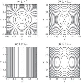
tension and pressure forces can balance each other, for instance in hyperbolic X-points. These two simple cases are sketched in Figure 1.7, and will be the basis for our two-dimensional relaxation experiments.
If the magnetic field is embedded in a plasma, the pressure force can hold a non-zero Lorentz force in a magnetohydrostatic equilibrium. In this case, we can define the (non-dimensional) plasma beta,β, as the ratio of the gas pressure to the magnetic pressure,
β= gas pressure plasma pressure =
p B2/2µ, hence
β= 2µp
B2 . (1.2.36)
(a) Homogeneous field
P = 0B T = 0B
(b) Hyperbolic X-point
TB PB
PB
PB
PB
TB
TB
TB
B=0
0.5 1.0
0.0 0.5
1.0
1.0 0.5 0.0 0.5 1.0 x
y
0.5 1.0
0.0 0.5
1.0
1.0 0.5 0.0 0.5 1.0 x
y
Figure 1.7: Two different configurations for magnetostatic equilibria. (a) Straight magnetic field,B=B0(0,1,0), with zero magnetic pressure forcePB and magnetic tensionTB, and (b) hyperbolic X-point,B =−B0(y, x,0), withPB = −TB at every point. In (b), the magnetic field contains a magnetic null point, whereB = 0, at the
origin.
effects, and whether they can be neglected or not. In general terms, most of the studies of coronal magnetic fields
assumeβ = 0, as the densities of the solar corona are extremely low. However, lower in the chromosphere and near locations where the magnetic field is very weak, or zero, this assumption is no longer valid.
1.3
MHD equilibria: Magnetohydrostatics
Magnetic fields in the solar atmosphere change continuously, and together with the solar plasma, they form a
highly dynamic environment. However, understanding MHD equilibrium conditions is extremely important for studying these complex hydromagnetic scenarios, for various reasons. Firstly, the set of MHD equations described
above has an immense degree of complexity, and so, studying the associated stationary states provides a much simpler solution to start with. Secondly, for every analytical and numerical study, it is essential to understand the
initial equilibrium state, depending on the demands of the study. Also, in relaxation-type experiments, one needs to know and understand the properties of the final states, whose mathematical descriptions must be provided by
the MHD equilibrium theory. Lastly, from the point of view of modelling, many of the physical processes studied
in solar plasma physics occur slowly, i.e. on time-scales much longer than the typical time-scale of the system, so the evolution of these systems can be modelled with a sequence of static equilibria. As an example, Schindler and
Birn (1986) used this quasi-static theory to model the dynamics of the Earth’s magnetotail.
The theory of the static solutions of the equations of MHD is called magnetohydrostatics (MHS). For such a
state, there are no macroscopic velocities and the dependence with time disappears. The equations and derivations shown in this section, including more general cases, are explained in detail in Edenstrasser (1980b,a). They are
also discussed by Priest (1982) and Biskamp (1993) “Nonlinear magnetohydrodynamics”.
fundamental equation of MHS,
j×B−∇p= 0, (1.3.1)
which can be rewritten using Amp`ere’s law (1.2.25), as
∇p= 1
µ(∇×B)×B. (1.3.2)
The very first result of magnetohydrostatics comes directly from equation (1.3.1), and is that the dot product of Band∇pis zero,
B·∇p= 0, (1.3.3)
so the only spatial changes in the pressurepmust be perpendicular to the magnetic field. In other words, in any static equilibrium, the plasma pressure is constant along field lines.
Combining the vector identity∇·(∇×A) = 0and the solenoidal constraint (1.2.26), the magnetic fieldB can be written as the curl of the vector potentialA, perpendicular to the magnetic field, where
B=∇×A. (1.3.4)
1.3.1
MHS equilibria in 2D
In a system with a translational invariance such as∂/∂z= 0(this is usually referred as to two and a half dimen-sions), we can rewriteBas
B=∇Az(x, y)×ez+Bz(x, y)ez, (1.3.5)
whereAzis thez-component of the vector potentialA. The scalar product ofBand∇Azequals zero,
B·∇Az = (∇Az×ez)·∇Az+Bzez·∇Az= 0, (1.3.6)
since the first term on the right hand side of (1.3.6) is the scalar product of two orthogonal vectors, and the second term is zero since∂Az/∂z = 0. Hence, in two (and two and a half) dimensions,Az is constant along magnetic
field lines. This is a big advantage, as, in fact, the contours ofAz are the projections of the magnetic field lines
onto thexy-plane. The functionAz(x, y)is known as the flux function.
Using equations (1.3.3) and (1.3.5), we get
B·∇p= (∇Az×ez)·∇p+Bzez·∇p= 0. (1.3.7)
Again,p=p(x, y), so the second term on the right of equation (1.3.7) is zero. Hence, the first term on the right hand side must be zero, and expanding it in terms of partial derivatives, we obtain
∂Az
∂y ∂p ∂x −
∂Az
which implies that the pressurepis a function of the flux functionAz,
p=F(Az), (1.3.8)
whereFis an unknown function that is dependent on the initial conditions and evolution.
Now, in a strictly two-dimensional system, the magnetic field components are given by
Bx=
∂Az
∂y , By=− ∂Az
∂x , Bz= 0, (1.3.9)
and both the vector potentialAand the current densityjhave an only non-zeroz-component, i.e.A=Azezand
j=jzez. The curl of the magnetic field is then given by
∇×B= (0,0,−∂
2A
z
∂y2 −
∂2Az
∂y2 ) =−∇ 2A
zez,
so that, from Amp`ere’s law (1.2.25), we get
jz=−1
µ∇
2A
z. (1.3.10)
Now, substituting (1.3.9) into equation (1.3.2), we obtain
∇p=−1
µ0∇ 2A
z∇Az,
and since∇p=∇Azdp/dAz, we get dp
dAz
=−1
µ0∇ 2A
z=jz. (1.3.11)
This is the Grad-Shafranov equation, for two-dimensional magnetic fields. Finally, combining equation (1.3.11)
with (1.3.8), we get
jz=F′(Az) = dF
dAz
. (1.3.12)
Equations (1.3.8) and (1.3.12) tell us that, for two dimensional fields in equilibrium, the plasma pressure and
current density are constant along field lines. This Grad-Shafranov equation gives the relation between these two quantities, and uniquely characterises a 2D MHS equilibrium.
1.3.2
Classification of the MHS equilibria
Looking at the fundamental equation of MHS (1.3.1), the equilibria can be classified into three different types,
Potential fields
A magnetohydrostatic equilibrium is said to be potential if there exists no current density, i.e. j = 0. Thus the Lorentz force, j×B, is zero, and in order to satisfy equation (1.3.1), the plasma pressure force must also equal zero. Amp`ere’s law (1.2.25) gives
∇×B= 0,
and from the vector identity∇×(∇φ) = 0, the solution for potential fields is given byB=∇φ, whereφ(x, y, z) is the scalar magnetic potential. Using the solenoidal constraint (1.2.26), we get
∇2φ= 0. (1.3.13)
Equation (1.3.13) is Laplace’s equation. Solutions can be obtained by various methods including separation
of variables, and are uniquely determined by the boundaries of the system. Hence, given an initial magnetohy-drodynamic system where the normal components to all boundaries are prescribed and fixed, subject to “external”
disturbances, there exists one and only one potential equilibrium.
Force-free fields
If both the gradient of pressure and the Lorentz force are zero, the equilibrium is known as force-free,
j×B= 0. (1.3.14)
Notice, that the potential fields are one particular solution of this. Equation (1.3.14) implies that in the force-free case, the current density vector is parallel to the magnetic field, and from Amp`ere’s law (1.2.25),
∇×B=αB, (1.3.15)
whereαmay be a function of position,r. Ifα= 0, the equilibrium is potential. From the vector identity∇·(∇×B) = 0, we have
∇·(αB) =α∇·B+B·∇α= 0,
and using the solenoidal constraint (1.2.26), we can get a restriction for the scalar functionα(r),
B·∇α= 0. (1.3.16)
Hence,αis constant along field lines, although it may vary from field line to field line. Taking the curl of equation (1.3.15), we get
∇×(∇×B) =∇×(αB)
=α(∇×B) +∇α×B =α2B+∇α×B,