December 20, 2017
Influence of galactic arm scale dynamics on the molecular
composition of the cold and dense ISM
I. Observed abundance gradients in dense clouds
M. Ruaud
12, V. Wakelam
2, P. Gratier
2, and I. A. Bonnell
31 NASA Ames Research Center, Moffett Field, CA, USA
2 Laboratoire d’astrophysique de Bordeaux, Univ. Bordeaux, CNRS, B18N, allée Geoffroy Saint-Hilaire, 33615 Pessac, France
3 Scottish Universities Physics Alliance (SUPA), School of Physics and Astronomy, University of St. Andrews, North Haugh,
St Andrews, Fife KY16 9SS, UK
Received September 15, 1996; accepted March 16, 1997
ABSTRACT
Aims.We study the effect of large scale dynamics on the molecular composition of the dense interstellar medium during the transition
between diffuse to dense clouds.
Methods.We followed the formation of dense clouds (on sub-parsec scales) through the dynamics of the interstellar medium at galac-tic scales. We used results from smoothed pargalac-ticle hydrodynamics (SPH) simulations from which we extracted physical parameters that are used as inputs for our full gas-grain chemical model. In these simulations, the evolution of the interstellar matter is
fol-lowed for∼50 Myr. The warm low-density interstellar medium gas flows into spiral arms where orbit crowding produces the shock
formation of dense clouds, which are held together temporarily by the external pressure.
Results.We show that depending on the physical history of each SPH particle, the molecular composition of the modeled dense clouds presents a high dispersion in the computed abundances even if the local physical properties are similar. We find that carbon
chains are the most affected species and show that these differences are directly connected to differences in (1) the electronic fraction,
(2) the C/O ratio, and (3) the local physical conditions. We argue that differences in the dynamical evolution of the gas that formed
dense clouds could account for the molecular diversity observed between and within these clouds.
Conclusions.This study shows the importance of past physical conditions in establishing the chemical composition of the dense medium.
Key words. Astrochemistry – ISM: clouds – ISM: evolution – ISM: kinematics and dynamics – ISM: molecules – Galaxy: evolution
1. Introduction
Observations of cold and dense interstellar clouds have revealed an extraordinary molecular richness, but also a large dispersion in the inferred abundances between and within these clouds. One of the most famous examples is given by the observation of the two low-mass cores TMC-1 and L134N for which more than 50 molecules have been identified (Bergin & Tafalla 2007;
Agún-dez & Wakelam 2013). Abundance gradients along the TMC-1
ridge were reported almost 40 years ago and their understand-ing has remained an unsolved problem since then. In this source, abundance gradients were observed along the ridge at scales of few 0.1 pc (Pratap et al. 1997). The southeastern end of the ridge (also known as the CP peak1) is characterized by enhanced abun-dances of carbon chains as compared to the northwestern end (also known as the NH3peak), while some other molecules (such
as NH3) are relatively well distributed along the ridge (Pratap
et al. 1997). For instance, HC7N/NH3ratio varies by more than
a factor of 30 along the ridge (Olano et al. 1988). At the CP peak position the inferred abundances of complex carbon chains are typically a factor of 10 higher than what is observed in the L134N dense cloud, which is thought to have similar physical properties as TMC-1 (Agúndez & Wakelam 2013). Even though
1 CP stands for cyanopolyyne here.
L134N do not show strong abundance variations on scales com-parable to TMC-1 (Dickens et al. 2000), small scale abundance gradients have also been revealed (on scales of few 0.01 pc) in the dense interior of this source, suggesting the presence of a pre-stellar core (Pagani et al. 2003,2004,2005).
In most cases, understanding these abundance gradients is a difficult task because, first, the chemistry is out of equilibrium in most of these objects and, second, molecular observations pro-vide us only a snapshot of their state. Although considerable the-oretical work has been conducted to understand the chemistry at work in such regions (e.g., Watson 1976; Herbst &
Klem-perer 1973;Prasad & Huntress 1980;Graedel et al. 1982;Leung
et al. 1984), most of the time dependent chemical modeling of
dense clouds relies on simple approximations that reflect these difficulties. Based on the lack of information on their dynami-cal state, dense clouds are often considered very simple objects in which the physical conditions are homogeneous and fixed. While such models have been shown to lead to relatively good agreement with observations in dense clouds (Wakelam et al.
2010;Agúndez & Wakelam 2013), they also have been highly
criticized. Most of these studies neglect the complex morphol-ogy of the source, often using a zero-dimensional approxima-tion (single point calculaapproxima-tion with homogenous and fixed phys-ical conditions). Such approximations can, of course, only be made up to a certain degree of spatial resolution (i.e., as revealed
by the careful analysis of L134N byPagani et al.(2003,2004, 2005)). Another critical point of these models is that they rely on a somewhat artificial choice of initial conditions (Gerin et al.
2003;Liszt 2009). A good example is given by the arbitrarily low
abundance of metals commonly used in these models. Graedel
et al. (1982) early recognized the need for lowering the
elec-tron abundance to better reproduce observations in some dense clouds. This has been achieved by decreasing the abundance of metals by a factor of∼ 100. This set of elemental abundances, known as low metal elemental abundances, are commonly used to model dense clouds and are aimed at taking into account the effect of the depletion during the transition between the diffuse and dense medium. However, the strength of the depletion used in this set of elemental abundances is somewhat arbitrary and does not rely on observational or theoretical constraints. One other important point discussed byLiszt(2009) is the absence of inherited molecules from the diffuse medium in the starting conditions of these models, for which all the elements are con-sidered to be in their atomic form except for hydrogen, which is usually considered to be in the form of H2. Indeed, while
dif-fuse clouds have long been thought to be devoid of molecules (which could have supported the assumptions described above), it is now clear that a wide range of molecules are present in the diffuse medium (e.g.,Snow & McCall 2006;Gerin et al. 2016). This is all the more important given that the use of these ini-tial conditions have raised the controversial idea of an early-time chemistry in dense clouds in which some objects may be seen in an early evolutionary stage. This so-called early-time chemistry is often invoked to explain the unusual large abundances of car-bon chains in TMC-1 (Herbst & Leung 1989;van Dishoeck et al.
1993).
These assumptions have also been questioned by recent hy-drodynamical simulations, which have brought new insights into the dynamic governing the formation of dense clouds (see, e.g.,
Hennebelle & Falgarone 2012; Dobbs et al. 2014; Klessen &
Glover 2016). These studies have profoundly changed our minds
about the very definition of what a dense cloud could be. Indeed all these studies show that rather than discrete objects, which could have been the case in the past, molecular clouds are con-stantly evolving objects that show a strong coupling with their environment (Klessen & Glover 2016). Although much effort has been made to couple the chemistry and dynamics, most hy-drodynamical modeling of the formation of molecular clouds in-cludes a very simple chemistry consisting of few elements and reactions (e.g.,Bergin et al. 2004;Glover et al. 2010;Clark et al. 2012). While this can be easily understood considering the com-putational requirements of such simulations, the impact of the dynamical evolution of the medium on the molecular content of dense clouds is poorly constrained and focuses on simple poly-atomic molecules and ions (Glover et al. 2010;Clark et al. 2012). Some studies have proposed overcoming this limitation by computing the chemistry as a post-treatment of hydrodynam-ical simulations (Hassel et al. 2010; Hincelin et al. 2013). Such hybrid models allow the use of complex chemical mod-els, which include several hundreds of chemical species coupled, through thousands of reactions, with outputs from complex high-resolution hydrodynamical simulations.
In this study, we adopt such technique to follow the evolu-tion of the chemical composievolu-tion during the formaevolu-tion process of dense clouds from the diffuse medium. To do so, we follow the formation of dense clouds (on sub-parsec scales) through the dynamics of the interstellar medium at galactic scales using re-sults of SPH smoothed particle hydrodynamics (SPH) simula-tions fromBonnell et al.(2013). We then post-process these
re-sults with our full gas-grain chemical model Nautilus (Ruaud
et al. 2016) to get the evolution of the chemical composition.
The main difference from the other more classical approaches to studying the chemical composition of dense clouds is that we do not make any assumptions about the initial composition of the dense cloud and let the chemical model evolve continuously from the diffuse to the dense interstellar medium.
The paper is organized as follows. In Section2we give an overview of the hydrodynamical simulations that we use, and present our cloud selection and our chemical model Nautilus. In Section 3we present the results obtained for the two dense clouds that we selected. In Section4we discuss these results and propose an analogy with what is observed and Section5contains a summary of our work.
2. Method
2.1. Hydrodynamical simulations overview
The numerical simulations ofBonnell et al.(2013) uses a three-dimensional SPH method to follow the gas dynamics in a galac-tic potential including spiral arms. A top-down approach is used to probe successive smaller scales from the scale of a spiral galaxy to the scale of dense cloud formation. In an initial simula-tion, the full galactic disk dynamics is followed over a period of
∼360 Myr. This simulation uses 2.5×10⁷SPH particles to model
109Mof gas in an annulus 5 to 10 kpc. A high-resolution sim-ulation is then performed for the last 54 Myr of the full disk evo-lution. This simulation was performed by selecting a 250×250 pc2region at the end of the full disk simulation and by splitting
original SPH particles into 256 lower mass particles. For this simulation, the selected region was traced backward through 54 Myr to produce the initial conditions for the high-resolution re-simulation. The selected region contains 1.09×10⁷SPH particles with an individual particle mass of 0.156 M. In this paper we focus on high-resolution re-simulations and definet = 0 Myr as the starting time of the simulation such that this time corre-sponds to t = 310 Myr of the full disk simulation (see Fig. 1 and 2 ofBonnell et al. 2013). In the selected high-resolution re-simulation region, gas from the spiral arm is cold (Tgas . 100 K) and dense (nH & 100 cm−3), whilst gas entering comprises warm gas (Tgas & 8000 K) and some cooler and denser gas
from previous spiral arm encounters. Dense clouds are formed by converging flows induced by shocks when the matter enters the spiral arm potential. At each shock, the gas is compressed and cools while maintaining pressure equilibrium with the sur-rounding warm gas (Bonnell et al. 2013). Self-gravity is not in-cluded in these simulations such that if the external pressure de-creases, the cool gas can re-expand and warm up.
2.2. Cloud selection and physical history
We performed cloud selection on the results obtained in the high-resolution re-simulation. This selection was carried out by first selecting a high density SPH particle in the dense cloud regime (typically withnH>105cm−3). The cloud was subsequently
de-fined by looking at all the particles passing in a radius≤0.5 pc of the position of this first selected particle at its maximum den-sity. The selected clouds are composed of few 102SPH particles
The visual extinctionAVhas been estimated using the stan-dard conversion from the total hydrogen column density,NH =
N(H)+2N(H2) (Bohlin et al. 1978;Rachford et al. 2009), written
as
AV= RV CD
NH
1 cm−2
!
, (1)
whereRV=3.1 andCD=5.8×1021cm−2mag−1. In a standard estimation ofAV, the knowledge ofNHrequires a selected a line of sight on which the integration overnH is made. In our case, AVis estimated for each SPH particle by assumingNH =hnH, wherehis the smoothing length of the considered SPH particle. The dust temperature is computed by the chemical model following the approach presented in Hollenbach et al.(1991). Dust absorption Qabswas taken fromDraine & Lee(1984) for 0.1µm silicate grains. The considered interstellar radiation field is composed by (1) the UV background (taken fromMathis et al. 1983), (2) the infrared emission from dust, and (3) the cosmic microwave background. The infrared emission spectrum from dust was taken fromDraine & Li(2007) and corresponds to the model withRV =3.1,qPAH =4.6% andχ =1. Using this ap-proach the dust temperature ranges betweenTdust ≈16K in un-shielded environment andTdust≈10K whenAV ≈10.
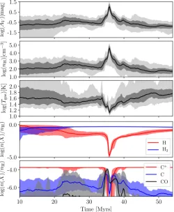
Figures1 and2 illustrate this selection for one cloud (de-noted as cloud A in the following) composed of∼250 SPH par-ticles. Figure1 presents the evolution of the total column den-sity map integrated along thez-axis (i.e., its morphology) of the cloud att =35.35 Myr,t =35.58 Myr, andt=35.82 Myr, re-spectively. The last map (i.e., att =38.82 Myr) corresponds to the peak density of the cloud on which the selection was made. Figure2presents the statistics associated with the evolution of the physical parameters extracted for all the SPH particles that compose this cloud and their evolution as a function of time. It also presents the computed evolution of H, H2, and C+, C, CO,
which are discussed in more detail in Section3. As shown in Fig.2, the cloud dissipates after the peak density is reached. As previously discussed, this comes from the fact that self-gravity is not taken into account in these simulations. In the following, we only focus on all the phases upstream of the cloud dissipation and ignore the downstream phases.
2.3. Post-processed chemistry
Each physical history was then used as an input for our gas-grain chemical model Nautilus (Ruaud et al. 2016). In this model, we computed the abundance of each species by solving a set of rate equations for gas-phase and grain-surface chemistries. The chemical network used is based on kida.uva.2014(
Wake-lam et al. 2015a) and includes the chemical schemes for carbon
chains proposed byWakelam et al.(2015b);Loison et al.(2016);
Hickson et al.(2016) and the update of the sulfur chemistry
net-work presented inVidal et al.(2017). This model computes the abundance of∼900 chemical species (∼600 for the gas phase and∼300 for the grain surface) that are coupled through more than 12 000 reactions. Gas-phase and grain-surface chemistries are connected via accretion and desorption. For grain chem-istry the model was used in its three-phase configuration, which means that a distinction is made between the surface layers (with at most two monolayers of adsorbed molecules) and the bulk. In this model, the surface and bulk are considered as chemically active and we assume that the bulk diffusion is driven by the diffusion of water molecules (seeRuaud et al. 2016, for a com-plete presentation of the model). Finally, grains are considered
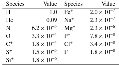
Species Value Species Value
H 1.0 Fe+ 2.0×10⁻⁷
He 0.09 Na+ 2.3×10⁻⁷
N 6.2×10⁻⁵ Mg+ 2.3×10⁻⁶
O 3.3×10⁻⁴ P+ 7.8×10⁻⁸
C+ 1.8×10⁻⁴ Cl+ 3.4×10⁻⁸
S+ 1.5×10⁻⁵ F 1.8×10⁻⁸
[image:3.595.331.527.58.165.2]Si+ 1.8×10⁻⁶
Table 1.Initial abundances.
Cloud A Cloud B
Number of SPH particles 237 287
Total mass (M)a 37 45
Mean radius (pc) 0.33 0.29
Velocity dispersion (km.s−1) 1.4 0.7
Virial parameterb 20.0 4.0
MedianTgas(K) 12.0 11.0
MediannH(cm−3) 4×10⁴ 7×10⁴
Table 2.Physical parameters of the two clouds considered in this study. These parameters are those obtained at the peak density of each clouds.
a The total mass is obtained by multiplying the number of SPH
par-ticles that compose each cloud by the individual particle mass 0.156
M.b The virial parameter of each cloud has been estimated byα =
5σ2
vR/GM(Bertoldi & McKee 1992).
to be spherical with a 0.1µm radius and a dust-to-gas mass ra-tio of 0.01. For all the chemical models presented throughout this paper, we used initial abundances relevant for diffuse cloud conditions. Initial abundances are listed in Table1 and corre-spond to abundances observed towardζOph (v=−15 km.s−1) listed inJenkins(2009). These initial conditions differ from the low-metal abundances typically used in pseudo-time-dependent chemical models in several aspects. Firstly, no assumptions were made about the depletion of metals and their abundances are higher by at least 2 dex as compared to Graedel et al.(1982). Secondly, the initial abundances of N, O, and C+are higher by 0.45 dex, 0.27 dex and 0.4 dex, respectively, leading to an initial C/O ratio of≈0.55. The cosmic ray ionization rate was taken to be equalζH2=1.3×10
−17s−1.
3. Results
In the following, we focus on two dense clouds (i.e., clouds A and B) among our selection. The selection of these two clouds has been motivated by (1) the similarity of the physical param-eters in the dense cloud regime, (2) the observed difference in the physical parameters in the phases that precede their forma-tion, and (3) the fact that they illustrate the two most extreme case of all the selected clouds. Table2summarizes the physical parameters of each cloud at their peak density.
3.1. General results illustrated in the example of the typical cloud A
x[pc]
y
[p
c]
t= 35.35 Myr
0.2 pc
21.0 21.0
21.5 21.5
x[pc]
t= 35.58 Myr
0.2 pc 21.0
21.5
22.0
x[pc]
t= 35.82 Myr
0.2 pc 21.0
21.5 22.0
20.50 21.00 21.50 22.00 22.50 23.00
log
(
NH
[image:4.595.94.503.62.199.2])
Fig. 1.Evolution of the total column density map of the cloud (denoted as cloud A in the following) att=35.35 Myr,t=35.58 Myr, andt=38.82
Myr, respectively. This cloud is formed by≈250 SPH particles and dissipates aftert≈36 Myr.
-1.5 -0.5 0.5 1.5
log
(
AV
)[mag]
1.0 2.0 3.0 4.0 5.0
log
(
nH
)[cm
3]
10 20 30 40 50
Time [Myrs] 1.0
1.2 1.4 1.6 1.8 2.0
log
(
Tgas
)[K]
-5.0 0.0
log
(
n
(
X
)
/n
H
)
H H2
10 20 30 40 50
Time [Myrs] -6.0
-4.0
log
(
n
(
X
)
/n
H
)
C+
[image:4.595.42.293.252.557.2]C CO
Fig. 2.Statistics associated with the evolution of the physical parame-ters of all SPH particles that compose cloud A. For the three first plots, the black line shows the evolution of the median of the physical param-eters. The dark gray filled area shows the 16th and 84th percentiles and the light gray filled area indicates the 2nd and 98th percentiles of the distribution. For the last two plots, the lines show the evolution of the median of the abundances while the filled area shows the 16th and 84th percentiles of the distribution.
that precede the formation of the dense cloud, most of the SPH particles have typical diffuse and translucent gas physical con-ditions (following the classification of Snow & McCall 2006). Betweent=0 andt=33 Myr, the median density isnH≈100 cm−3, the median gas temperature isTgas≈40 K, and the median visual extinction isAV ≈0.2 mag (as shown in Fig.2, it is
im-portant to note the large dispersion around these values). In this simulation, the H-H2transition occurs aroundt≈15 Myr. After
this time, the molecular fraction, fH2 =2n(H2)/[n(H)+2n(H2)]
, slowly increases from fH2 ≈ 0.5 to a plateau of fH2 ≈ 0.9 at
t≈25 Myr, wherenH≈300 cm−3 until it reachesfH2 ≈1 when
nH&104cm−3, such that H is mostly in the form of H
2when the
dense cloud begins to form aroundt = 33 Myr. The transition between C+, C, and CO occurs att≈34.7 Myr, wherenH≈103 cm−3. After this time, the carbon is mostly in the form of CO.
As shown in Fig.2, aftert≈35.4 Myr the gas-phase CO signif-icantly decreases and starts to deplete severely at the surface of the grains, whereAV&7 mag andnH&104cm−3.
3.1.1. Spatial distribution of commonly observed gas-phase molecules
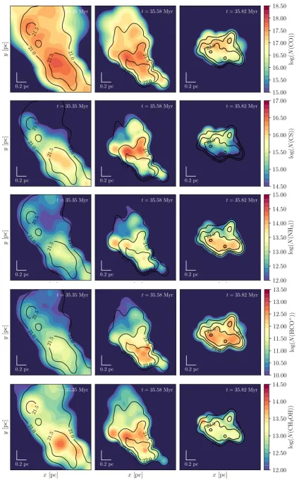
Fig.3presents the computed column density maps of CO, CS, NH3, HCO+, and CH3OH at t = 35.35 Myr, t = 35.58 Myr,
andt = 35.82 Myr for cloud A. Contour lines were added for clarity and indicate log(NH) ranging from 21 to 23. These com-puted column densities are in general in good agreement with what is observed in dense clouds presenting similar total col-umn density. Att=35.35 Myr most of the molecules shown in this figure follow the distribution ofNH. As discussed before, the gas-phase CO, as well as CS here, starts to severely deplete onto grains (this mechanism is also called the freezing out) around
t = 35.40 Myr, leading to a decrease of their gas-phase abun-dance. This freeze-out leads to an abundance gradient of these molecules along the north-south direction when the cloud has reached its peak density. On the contrary, NH3and CH3OH are
well distributed in the entire cloud and roughly follow the dis-tribution ofNH. Such selective depletion is commonly observed in pre-stellar cores (e.g.,Willacy et al. 1998;Caselli et al. 1999;
Bergin et al. 2002;Bacmann et al. 2002;Tafalla et al. 2004;
Lip-pok et al. 2013). Authors such asWillacy et al.(1998),Tafalla
et al.(2004), orPagani et al.(2005) have shown that in several
sources, molecules such as CO, CS, CCS, or SO are strongly depleted in core interiors, while species such as N2H+and NH3
show almost no signs of depletion. As suggested by previous models (e.g.,Bergin & Langer 1997) and observations, we find that the depletion of CO and CS is triggered by the local density of each SPH particle. The homogeneity of the spatial distribu-tion of NH3and CH3OH is found to be closely linked with their
grain surfaces allow their continuous replenishment of the gas phase, which explain the homogeneity of their spatial distribu-tion.
3.1.2. Grain surface chemistry and ice composition
For this cloud, we found that the first monolayer of ice is formed aroundt ≈34.5 Myr, whereTdust ≈13 K,nH ≈103 cm−3 and AV ≈ 1.3 mag. This value is very close to the typical thresh-old observed in the interstellar mediumAV≈1.6 (Whittet et al.
2001;Boogert et al. 2015). At this time, the low dust
tempera-ture, which ensures a relatively low rate of thermal desorption of most of the molecules present on the surface, and the significant shielding by dust, which ensures a low rate of photodesorption, allow molecules to stay physisorbed on grains and the mantle to grow. As suggested by the observations (see Boogert et al. 2015, for a review on observations of interstellar ices), we found that the few first monolayers of ice are polar ices2and that they mainly consist of H2O (≈ 80% of the total ice material), NH3
(≈ 11% of the total ice material), and CH4 (≈ 3% of the total
ice material). At this time, these three molecules are found to be formed by successive hydrogenation of atomic oxygen3, nitro-gen, and carbon on grain surfaces, respectively.
At the peak density of the cloud, i.e., att ≈ 36 Myr,nH ≈
4×104 cm−3,T
gas ≈ 12 K, and AV ≈ 10 mag, a thickness of ≈100 monolayers of ice is reached. H2O is found to be the main
constituent of the ice (≈ 40% of the total ice material). Other contributions come from CO (≈25% with respect to H2O for its
median abundance), CO2, CH4, HCOOH (≈ 10% each), NH3,
N2, HS (≈8% each) H2S, CH3OH (≈6% each), CH2NH2, HCN,
H2CO (≈2% each), and CH3O, HCO, ... (.2% each). The
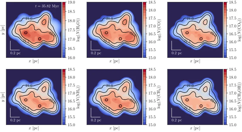
com-puted column densities of the main observed grain species at the peak density of the cloud are shown in Fig.4.
3.2. The case of one particular cloud: Cloud B
In this section, we present results obtained for one particular cloud for which we observe strong abundance gradients within the cloud (denoted as cloud B). The evolution of the morphology of the cloud is shown in Fig.5, fromt=45.48 Myr tot=45.96 Myr. The statistics associated with the evolution of the physical parameters of all the SPH particles that compose this cloud are shown in Fig.6. As in the case of cloud A, all the SPH particles that compose this cloud have diffuse and translucent gas phys-ical conditions in the phases that precede the formation of the cloud. Similar to the previous cloud, the H-H2transition occurs
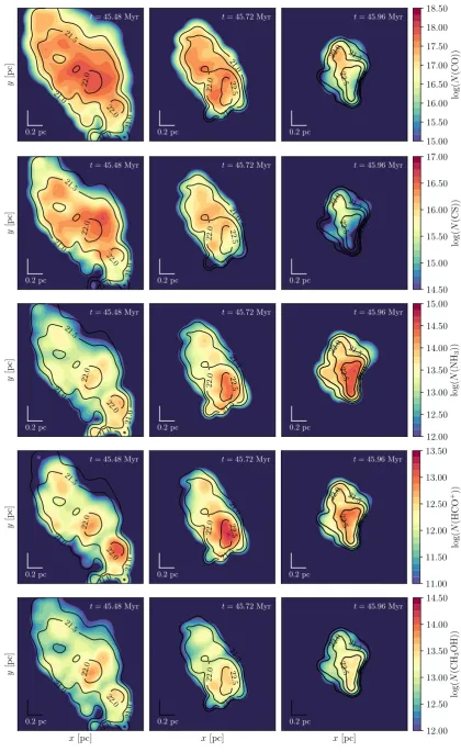
well before the dense cloud begins to form; i.e.,t≈20 Myr, and we have fH2 ≈ 1 in the dense cloud regime. Fig. 7shows the computed column density maps of CO, CS, NH3, HCO+, and
CH3OH att=45.48 Myr,t=45.72 Myr, andt=45.96 Myr. As
in the case of cloud A we find that CO and CS start to severely deplete aroundt ≈ 45.7 Myr. This also leads to an abundance gradient of these molecules along the northeast–southwest di-rection in the cloud, while NH3and CH3OH closely follow the
distribution ofNH.
2 In general the different type of ices, i.e., H
2O rich and CO rich, are
referred to polar and apolar ices due to the different molecular dipole
moments. Apolar ices are dominated by molecules with low dipole
mo-ments (e.g., CO, N2) that have relatively low sublimation temperatures
(Boogert et al. 2015).
3 We note that, as already mentioned, for this cloud the transition from
C+to CO occurs att≈34.7 Myr, such that most of the oxygen is mainly
in its atomic form when the first monolayers of ice start to form.
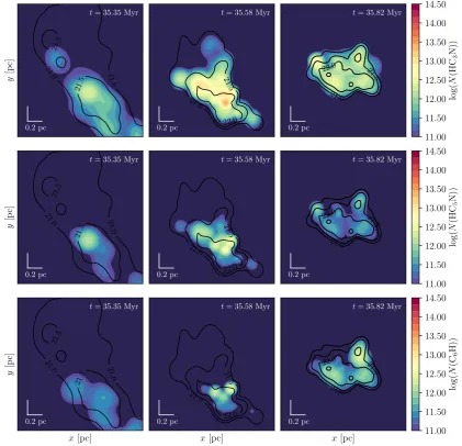
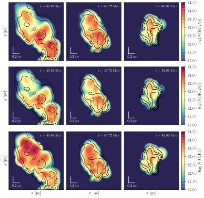
Although the physical parameters in the densest region of this cloud are relatively similar to that of cloud A, we observed that the presence of an intermediate density pre-phase (i.e., for which nH ranges between few 102 cm−3 and few 104 cm−3) around t ≈ 43 Myr strongly affects the predicted abundances of several molecules in the cold dense cloud regime. These dif-ferences are mostly found for carbon chains that are present at high column densities in cloud B. Figs.8and9present a com-parison of the computed column density map of HC3N, HC5N,
and C6H for clouds A and B. In addition to the fact that we find
column densities of carbon chains∼10 times higher in cloud B than in cloud A, we also find that carbon chains show a relatively high dispersion in their abundances as compared to cloud A.
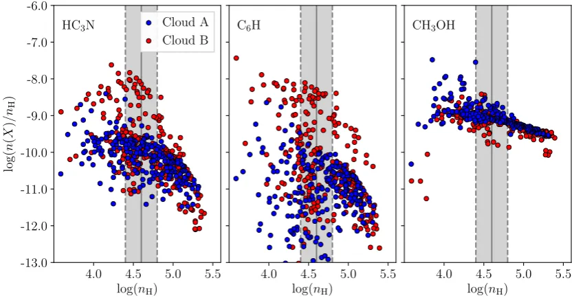
This dispersion is illustrated in Fig.10, which presents the abundance of three molecules, HC3N, C6H, and CH3OH, as a
function of the local density of each SPH particle at the peak density of each cloud. As shown in this figure, whilst for CH3OH
the results for both clouds are similar and show very little dis-persion, the results obtained for HC3N and C6H show a
signif-icant dispersion (of at least 2 and 3 dex for HC3N and C6H,
respectively at nH = 4 ×104 cm−3). It is also important to
note that this dispersion is larger in the case of cloud B, which shows enhanced abundances of these two molecules for some SPH particles; those particles with enhanced abundances are im-portant because they are responsible for the high column den-sity of these molecules. More generally, Fig.11presents all the gas-phase molecules with abundances greater than 10−11 that
present a difference greater than 1.5 dex from the abundances be-tween the 16th and 84th percentile in a range of 0.2 dex around log(nH) = 4.6, at the peak density (i.e., as shown by the dark shaded area in Fig. 10) of each cloud. The choice to restrain the density interval on which the dispersions are calculated is to try to remove the dependency on the local density of each parti-cles and thus dispersion caused by the depletion on grains. The fact that this strong dispersion in the HC3N and C6H abundances
(and more generally all the molecules presented in Fig.11) can be observed at a given density suggests that this dispersion is not only due to local physical conditions (e.g., adsorption on grain surface), but to the physical history that each particle underwent before reaching this time. As shown in Fig.11, most of these species are carbon chains. In this range of densities, the most important dispersion in the abundances is observed for complex carbon chains species that can be as high as four orders of mag-nitude for both clouds.
From these results, at least three major questions arise: (1) What causes this dispersion? (2) Why are carbon chains the most affected? and (3) What explains the observed enhancement of carbon chains in cloud B as compared to cloud A? We try to answer these three questions in the following by focusing on the results obtained in cloud B.
3.3. Link with physical history and local physical conditions
In general, we find that this dispersion in the abundances ob-served in cloud B is strongly correlated to the electronic fraction of the medium, gas-phase C/O ratio, and local density of each SPH particle.
x[pc]
y
[p
c]
t= 35.35 Myr
0.2 pc
21.0 21.0
21.5 21.5
x[pc]
t= 35.58 Myr
0.2 pc 21.0
21.5
22.0
x[pc]
t= 35.82 Myr
0.2 pc 21.0
21.5 22.0
15.00 15.50 16.00 16.50 17.00 17.50 18.00 18.50
log
(
N
(CO))
x[pc]
y
[p
c]
t= 35.35 Myr
0.2 pc
21.0 21.0
21.5 21.5
x[pc]
t= 35.58 Myr
0.2 pc 21.0
21.5
22.0
x[pc]
t= 35.82 Myr
0.2 pc 21.0
21.5 22.0
14.50 15.00 15.50 16.00 16.50 17.00
log
(
N
(CS))
x[pc]
y
[p
c]
t= 35.35 Myr
0.2 pc
21.0 21.0
21.5 21.5
x[pc]
t= 35.58 Myr
0.2 pc 21.0
21.5
22.0
x[pc]
t= 35.82 Myr
0.2 pc 21.0
21.5 22.0
12.00 12.50 13.00 13.50 14.00 14.50 15.00
log
(
N
(NH
3
))
x[pc]
y
[p
c]
t= 35.35 Myr
0.2 pc
21.0 21.0
21.5 21.5
x[pc]
t= 35.58 Myr
0.2 pc 21.0
21.5
22.0
x[pc]
t= 35.82 Myr
0.2 pc 21.0
21.5 22.0
10.00 10.50 11.00 11.50 12.00 12.50 13.00 13.50
log
(
N
(HCO
+ ))
x[pc]
y
[p
c]
t= 35.35 Myr
0.2 pc
21.0 21.0
21.5 21.5
x[pc]
t= 35.58 Myr
0.2 pc 21.0
21.5
22.0
x[pc]
t= 35.82 Myr
0.2 pc 21.0
21.5 22.0
12.00 12.50 13.00 13.50 14.00 14.50
log
(
N
(CH
3
[image:6.595.87.512.54.734.2]OH))
Fig. 3.Computed gas-phase column density maps of CO, CS, NH3, HCO+, CH3OH att=35.35 Myr,t=35.58 Myr andt=35.82 Myr for cloud
x[pc]
y
[p
c]
t= 35.82 Myr
0.2 pc 21.0 21.5 22.0 x[pc] 0.2 pc 21.0 21.5 22.0 x[pc] 0.2 pc 21.0 21.5 22.0 x[pc] y [p c] 0.2 pc 21.0 21.5 22.0 x[pc] 0.2 pc 21.0 21.5 22.0 x[pc] 0.2 pc 21.0 21.5 22.0
0.0 0.2 0.4 0.6 0.8 1.0
0.0 0.2 0.4 0.6 0.8 1.0
[image:7.595.92.506.59.285.2]0.0 0.2 0.4 0.6 0.8 1.0 16.0 16.5 17.0 17.5 18.0 18.5 19.0 log ( N (H 2 O)) 15.0 15.5 16.0 16.5 17.0 17.5 18.0 18.5 log ( N (CO)) 15.0 15.5 16.0 16.5 17.0 17.5 18.0 18.5 log ( N (CO 2 )) 15.0 15.5 16.0 16.5 17.0 17.5 18.0 18.5 log ( N (NH 3 )) 15.0 15.5 16.0 16.5 17.0 17.5 18.0 18.5 log ( N (CH 4 )) 15.0 15.5 16.0 16.5 17.0 17.5 18.0 18.5 log ( N (CH 3 OH))
Fig. 4.Computed column density map of H2O, CO, CO2, NH3, CH4, and CH3OH on grains at the peak density of cloud A (att=35.82 Myr).
Contours were added for clarity and indicates log(NH) from 21 to 23.
x[pc]
y
[p
c]
t= 45.48 Myr
0.2 pc 21.0 21.0 21.0 21.5 22.0 22.0 x[pc]
t= 45.72 Myr
0.2 pc 21.0 21.5 22.0 22.5 x[pc]
t= 45.96 Myr
0.2 pc 21.0 21.5 22.0 22.5 20.50 21.00 21.50 22.00 22.50 23.00 log ( NH )
Fig. 5.Evolution of the total column density map of cloud B. This figure shows the total column density of the cloud att=45.48 Myr,t=45.72
Myr, andt=45.96 Myr, respectively. This cloud is formed by≈300 SPH particles.
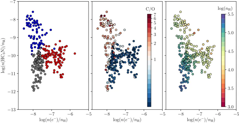
Given the size of the problem we first applied a principal compo-nent analysis (PCA;Jolliffe 2002) to reduce the dimensionality of the data set prior to clustering; a mean subtraction was per-formed over the data set before applying the PCA. This allowed us to validate the choice of the number of clusters that we used by making possible a direct visualization of the clustering re-sults in the subspace of principal components (PCs). We then checked that the clustering results using PCs and original data give similar results. The clustering using PCs att≈46 Myr was performed over the three first PCs, which contain more than 90% of the variation in the modeling results (≈70% for the first PC,
≈15% for the second, and≈6% for the third). Fig.12shows an example of the results obtained after clustering using PCs. These three plots present the abundance of HC3N as a function of the
electronic fraction of each SPH particle at the peak density of the cloud att ≈46 Myr. The left panel shows the result of the clustering obtained withk=3; the colors show the three clusters identified. The middle panel shows the same results but with a color coding that traces the C/O ratio computed just after the first density phase (i.e., att ≈ 44.5 Myr) and the right panel with a color coding that traces the individual density of each SPH parti-cle att≈46 Myr. It is important to note that the C/O ratio shown
here does not correspond to the ratio between atomic C and O, but the ratio over all the carbon and oxygen molecular species present in the gas phase at this time.
As shown in Fig.12, the first cluster in gray traces all the par-ticles with a low abundance of HC3N, a low electronic fraction
and a high local density (typicallynH&105cm−3). In this case, the high density of each of these particles explains both the low abundance of HC3N—and, more generally, all the molecules that
do not have efficient grain surface formation routes that could al-low their gas-phase replenishment—and the al-low electronic frac-tion (i.e., due to the accrefrac-tion of the electron donors at the surface of the grains).
The case of the two other clusters is interesting because even though they have roughly similar local physical conditions (as shown on the right panel of Fig.12for the local density of each SPH particle), these two clusters show very different behaviors. Indeed, as shown in Fig.12, the cluster in blue mostly traces all the particles with a high abundance of HC3N (this is also the
case for all the molecules presented in Fig.11), a low electronic fraction on the order ofn(e−)/n
H≈10−8, and a C/O ratio larger
[image:7.595.90.508.333.472.2]-1.5 -0.5 0.5 1.5
log
(
AV
)[mag]
1.0 2.0 3.0 4.0 5.0
log
(
nH
)[cm
−
3]
10 20 30 40 50
Time [Myrs] 1.0
1.2 1.4 1.6 1.8 2.0
log
(
Tgas
)[K]
Fig. 6.Statistics associated with the evolution of the physical parame-ters of all the SPH particles that compose cloud B. The black line shows the evolution of the median of the physical parameters. The dark gray filled area shows the 16th and 84th percentiles and the light gray filled area indicates the 2nd and 98th percentiles of the distribution.
electronic fraction, and C/O.1. In the case of this cluster, the abundance of HC3N and the electronic fraction are highly
cor-related with the local density of the medium and decrease as the density increases.
By tracing the history of each cluster back in time, we find that the low electronic fraction and high C/O ratio observed in the cluster in blue are directly connected to the passage of these particles in the intermediate density pre-phase around t = 43 Myr. This is illustrated in Fig.13, which shows the statistics of the physical parameters associated with each particle cluster.
For this cluster, we find that, firstly, this intermediate density pre-phase reduces the abundance of the main electron donors due to their accretion on grains and thus reduces the electronic fraction of the cloud, which is now controlled by the cosmic ray ionization of H2 and He. This is shown in Fig. 15, which
shows the abundance of metals (which represents the sum over C+, S+, Si+, Fe+, Na+, Mg+, P+, and Cl+) as a function of the electronic fraction of each particle cluster at the peak density of cloud (i.e., att ≈46 Myr). Secondly, this intermediate density pre-phase increases the gas-phase C/O ratio because of the for-mation of water ice on grain, which leads to a sequestration of atomic oxygen on grains. For this cluster, we find that almost 80 monolayers consisting of∼80% of water ice are present on the surface of the grains after this density phase. This means that for these SPH particles, a large amount of the elemental oxygen has been removed from the gas phase and included in the solid phase during this event.
These two effects have a strong impact on the formation of complex carbon chains. Indeed, carbon chains are mainly formed by ionic pathways and neutral-neutral reactions in which insertion of carbon atoms is a crucial step.
Therefore, on the one hand, by reacting with intermediate ions, electrons play an important role in setting this synthetic reaction chain mechanism efficiency (seeAgúndez & Wakelam 2013, for a complete review of the chemistry in dark clouds). Removing the main electron donors from the gas phase have the consequence of promoting the ion-neutral chemistry in the sense that intermediates are less destroyed by electronic recombina-tion.
On the other hand, the formation water ice on grains in-creases the amount of free carbon, which is otherwise mostly locked up into CO, that can be used for the synthesis of car-bon chains. However, as shown in the middle panel of Fig.12, a higher C/O ratio does not necessarily mean a higher abundance of complex carbon chains. This strongly depends on the amount of atomic and ionized carbon available and thus on the local physical conditions of each SPH particle. For this cluster, we find that this water rich ice survives until the cloud forms. How-ever, when looking at the spatial distribution of molecules in the cloud, we find that this does not produce observable constraints that could allow us to trace such history. This is illustrated in Figs.4and14, which present the computed column densities of the main observed grain species at the peak density of clouds A and B, respectively.
On the contrary, most of the particles in cluster red have not experienced such a high density pre-phase (or at least with a lower intensity). This results in an lower C/O ratio, meaning a lower abundance of free carbon, which is mostly locked up into CO, but also, as shown in Fig.15, a higher abundance of metals. This implies a relatively high electronic fraction, which prevents the efficient formation of carbon chains.
This link with the past history of each SPH particle also ex-plains the observed deficit of carbon chains in cloud A as com-pared to cloud B. Indeed, the fact that cloud A evolves continu-ously from the diffuse medium (i.e., without density pre-phase) to the dense cloud regime leads to a high electronic fraction (n(e−)/nH≈2×10−7att =35.82 Myr). As a consequence, by
reacting with intermediate ions, this high abundance of electrons prevents the formation of complex carbon chains in the cloud.
4. Discussion and analogy with observations of dense clouds
Several attempts have been made to explain the unusual high abundances of carbon chains observed in the TMC-1 dense cloud. One of the most popular scenarios relies on the so-called early time chemistry. This scenario is based on the fact that car-bon chain chemistry requires carcar-bon to be present in a reactive form in the gas phase. In pseudo-time-dependent models, this condition is satisfied at early time, i.e., before few 105years
af-ter which the carbon is locked up in CO (see Fig. 3 ofAgúndez &
Wakelam 2013, for exemple). In this scenario, molecular clouds
are thus considered to be seen in an early evolutionary stage in which the available carbon is still in an reactive form. Another possible explanation has been to invoke a different C/O ratio in TMC-1 as compared to other clouds (Bergin et al. 1996). In both case, the net effect of these scenarios is to increase the amount of free carbon that can be used for the synthesis of these molecules. Some authors have proposed a lower electronic fraction of TMC-1 as a good explanation of these unusual abundances. As discussed earlier, the effect of the electronic fraction on the synthesis of complex molecules has been early recognized by
Graedel et al.(1982) who proposed so-called low metal
abun-dances. However, it has been shown that the use of these low metal abundances could not itself explain the observed abun-dances of carbon chains in this cloud (seeAgúndez & Wakelam 2013, for exemple). Several others studies have tried to find some explanations for a possible lower electronic fraction in TMC-1 as compared to others clouds.Flower et al.(2007) for example showed that a lower cosmic ray ionization rate in TMC-1 could help explain the carbon chain abundances of this cloud, while
Wakelam & Herbst(2008) discussed the importance of PAHs on
x[pc]
y
[p
c]
t= 45.48 Myr
0.2 pc
21.0
21.0
21.0 21.5
22.0
22.0
x[pc]
t= 45.72 Myr
0.2 pc
21.0
21.5
22.0
22.5
x[pc]
t= 45.96 Myr
0.2 pc
21.0 21.5
22.0
22.5
15.00 15.50 16.00 16.50 17.00 17.50 18.00 18.50
log
(
N
(CO))
x[pc]
y
[p
c]
t= 45.48 Myr
0.2 pc
21.0
21.0
21.0 21.5
22.0
22.0
x[pc]
t= 45.72 Myr
0.2 pc
21.0
21.5
22.0
22.5
x[pc]
t= 45.96 Myr
0.2 pc
21.0 21.5
22.0
22.5
14.50 15.00 15.50 16.00 16.50 17.00
log
(
N
(CS))
x[pc]
y
[p
c]
t= 45.48 Myr
0.2 pc
21.0
21.0
21.0 21.5
22.0
22.0
x[pc]
t= 45.72 Myr
0.2 pc
21.0
21.5
22.0
22.5
x[pc]
t= 45.96 Myr
0.2 pc
21.0 21.5
22.0
22.5
12.00 12.50 13.00 13.50 14.00 14.50 15.00
log
(
N
(NH
3
))
x[pc]
y
[p
c]
t= 45.48 Myr
0.2 pc
21.0
21.0
21.0 21.5
22.0
22.0
x[pc]
t= 45.72 Myr
0.2 pc
21.0
21.5
22.0
22.5
x[pc]
t= 45.96 Myr
0.2 pc
21.0 21.5
22.0
22.5
11.00 11.50 12.00 12.50 13.00 13.50
log
(
N
(HCO
+))
x[pc]
y
[p
c]
t= 45.48 Myr
0.2 pc
21.0
21.0
21.0 21.5
22.0
22.0
x[pc]
t= 45.72 Myr
0.2 pc
21.0
21.5
22.0
22.5
x[pc]
t= 45.96 Myr
0.2 pc
21.0 21.5
22.0
22.5
12.00 12.50 13.00 13.50 14.00 14.50
log
(
N
(CH
3
[image:9.595.86.507.59.745.2]OH))
x[pc]
y
[p
c]
t= 35.35 Myr
0.2 pc
21.0 21.0
21.5 21.5
x[pc]
t= 35.58 Myr
0.2 pc 21.0
21.5
22.0
x[pc]
t= 35.82 Myr
0.2 pc 21.0
21.5 22.0
11.00 11.50 12.00 12.50 13.00 13.50 14.00 14.50
log
(
N
(HC
3
N))
x[pc]
y
[p
c]
t= 35.35 Myr
0.2 pc
21.0 21.0
21.5 21.5
x[pc]
t= 35.58 Myr
0.2 pc 21.0
21.5
22.0
x[pc]
t= 35.82 Myr
0.2 pc 21.0
21.5 22.0
11.00 11.50 12.00 12.50 13.00 13.50 14.00 14.50
log
(
N
(HC
5
N))
x[pc]
y
[p
c]
t= 35.35 Myr
0.2 pc
21.0 21.0
21.5 21.5
x[pc]
t= 35.58 Myr
0.2 pc 21.0
21.5
22.0
x[pc]
t= 35.82 Myr
0.2 pc 21.0
21.5 22.0
11.00 11.50 12.00 12.50 13.00 13.50 14.00 14.50
log
(
N
(C
6
[image:10.595.85.507.59.465.2]H))
Fig. 8.Computed gas-phase column density maps of HC3N, HC5N, and C6H for cloud A.
In this study we propose that the observed differences be-tween dense clouds may arise from different dynamical evolu-tion. We show that both the local physical conditions and the history of each SPH particle have an impact on the computed abundances of each dense clouds. We find that these differences mainly arise from (1) the electronic fraction, (2) the C/O ratio, and (3) the local physical conditions (i.e., the local density in our case). Although these mechanisms have already been invoked by previous studies, we show their direct link with the dynamics at large scale. This gives a more natural explanation of the observed differences between dense clouds but also within some of them. In particular, these results show that the often invoked early time chemistry is not a requisite to produce high abundances of car-bon chains. On the contrary, based on the results obtained with our cloud B, we show that high abundance of carbon chains can be the result of more evolved gas, i.e., having experienced a past density phase in this case.
In this context and by analogy with the observations, we ar-gue that the strong abundance gradients observed on sub-parsec scales in the TMC-1 dense cloud (Olano et al. 1988;Pratap et al. 1997) may originate from a different dynamical evolution of the gas that formed it. In particular, the observed enhancement of carbon chains in the so-called cyanopolyyne peak may, as in the
case of our cloud B, traces a past density phase in which most of the electron donors have been removed from the gas phase, en-hancing the ion-molecule chemistry. On the same basis, it could also explain the low abundance of carbon chains in the L134N dense cloud, which in this case would have a higher electronic fraction than TMC-1 and may be closer to our cloud A.
x[pc]
y
[p
c]
t= 45.48 Myr
0.2 pc
21.0
21.0
21.0 21.5
22.0
22.0
x[pc]
t= 45.72 Myr
0.2 pc
21.0
21.5
22.0
22.5
x[pc]
t= 45.96 Myr
0.2 pc
21.0 21.5
22.0
22.5
11.00 11.50 12.00 12.50 13.00 13.50 14.00 14.50
log
(
N
(HC
3
N))
x[pc]
y
[p
c]
t= 45.48 Myr
0.2 pc
21.0
21.0
21.0 21.5
22.0
22.0
x[pc]
t= 45.72 Myr
0.2 pc
21.0
21.5
22.0
22.5
x[pc]
t= 45.96 Myr
0.2 pc
21.0 21.5
22.0
22.5
11.00 11.50 12.00 12.50 13.00 13.50 14.00 14.50
log
(
N
(HC
5
N))
x[pc]
y
[p
c]
t= 45.48 Myr
0.2 pc
21.0
21.0
21.0 21.5
22.0
22.0
x[pc]
t= 45.72 Myr
0.2 pc
21.0
21.5
22.0
22.5
x[pc]
t= 45.96 Myr
0.2 pc
21.0 21.5
22.0
22.5
11.00 11.50 12.00 12.50 13.00 13.50 14.00 14.50
log
(
N
(C
6
[image:11.595.87.508.62.470.2]H))
Fig. 9.Same as Fig.8but for cloud B.
the presence of a localized source of radiation could be impor-tant enough to remove material from the surface of the grains after the intermediate density pre-phase (either by direct pho-todesorption or thermal evaporation of the ice if the temperature gets high enough) and thus significantly affect the results. In this case a proper modeling of the entire region would be required to track the evolution of the surrounding gas and thus the possibil-ity to form stars in the vicinpossibil-ity of the considered clouds.
5. Conclusions
In this study we used results from large scale hydrodynami-cal simulations to study the transition between diffuse to dense clouds on the molecular composition of the dense interstellar medium. We used results from SPH simulations byBonnell et al. (2013) from which we extracted physical parameters as a func-tion of time that have been used as inputs for our full gas-grain chemical model. Our results show that the molecular composi-tion of dense clouds show a high dispersion in the computed abundances and especially for carbon chains. We showed that be-sides the abundance gradient caused by the depletion on grains (triggered by the local density of each SPH particle), the his-tory of each SPH particle has a strong impact on the computed
abundances of carbon chains. Based on the results obtained for one particular cloud for which high column densities of carbon chains are found, we show that these differences arise from dif-ferences in (1) the electronic fraction (2) the C/O ratio, and (3) the local physical conditions (i.e., the local density of each SPH particle in our case). These differences are directly linked to a different dynamical evolution of the gas that formed the cloud for which some SPH particles went to an intermediate density pre-phase prior its formation. This intermediate density pre-pre-phase reduces the electronic fraction of the cloud, but also affects the C/O ratio which becomes larger than 1 due to the formation of water at the surface of grains. Based on these results, we pro-pose that the observed differences between dense clouds may arise from different dynamical evolution of the gas that formed these clouds.
Acknowledgements. This work has been founded by the European Research
4.0 4.5 5.0 5.5 log(nH)
-13.0 -12.0 -11.0 -10.0 -9.0 -8.0 -7.0 -6.0
log
(
n
(
X
)
/n
H
)
HC3N Cloud A
Cloud B
4.0 4.5 5.0 5.5 log(nH)
C6H
4.0 4.5 5.0 5.5 log(nH)
[image:12.595.87.505.60.277.2]CH3OH
Fig. 10.Computed gas-phase abundances of HC3N, C6H, CH3OH as a function of the local density of each SPH particle at the peak density of
cloud A and B, i.e., att=35.82 Myr andt=45.96 Myr, respectively. Points in blue are the results obtained for cloud A, while points in red show
the results obtained in the case of cloud B. The black line presents the median density of both clouds and the filled area indicates the range on
which the abundance dispersion of Fig.11was computed.
References
Agúndez, M. & Wakelam, V. 2013, Chemical Reviews, 113, 8710 Bacmann, A., Lefloch, B., Ceccarelli, C., et al. 2002, A&A, 389, L6 Bergin, E. A., Alves, J., Huard, T., & Lada, C. J. 2002, ApJ, 570, L101 Bergin, E. A., Hartmann, L. W., Raymond, J. C., & Ballesteros-Paredes, J. 2004,
ApJ, 612, 921
Bergin, E. A. & Langer, W. D. 1997, ApJ, 486, 316
Bergin, E. A., Snell, R. L., & Goldsmith, P. F. 1996, ApJ, 460, 343 Bergin, E. A. & Tafalla, M. 2007, ARA&A, 45, 339
Bertoldi, F. & McKee, C. F. 1992, ApJ, 395, 140
Bohlin, R. C., Savage, B. D., & Drake, J. F. 1978, ApJ, 224, 132 Bonnell, I. A., Dobbs, C. L., & Smith, R. J. 2013, MNRAS, 430, 1790 Boogert, A. C. A., Gerakines, P. A., & Whittet, D. C. B. 2015, ARA&A, 53, 541 Caselli, P., Walmsley, C. M., Tafalla, M., Dore, L., & Myers, P. C. 1999, ApJ,
523, L165
Clark, P. C., Glover, S. C. O., Klessen, R. S., & Bonnell, I. A. 2012, MNRAS, 424, 2599
Dickens, J. E., Irvine, W. M., Snell, R. L., et al. 2000, ApJ, 542, 870
Dobbs, C. L., Krumholz, M. R., Ballesteros-Paredes, J., et al. 2014, Protostars and Planets VI, 3
Draine, B. T. & Lee, H. M. 1984, ApJ, 285, 89 Draine, B. T. & Li, A. 2007, ApJ, 657, 810
Flower, D. R., Pineau Des Forêts, G., & Walmsley, C. M. 2007, A&A, 474, 923 Gerin, M., Fossé, D., & Roueff, E. 2003, in SFChem 2002: Chemistry as a
Diag-nostic of Star Formation, ed. C. L. Curry & M. Fich, 81
Gerin, M., Neufeld, D. A., & Goicoechea, J. R. 2016, ARA&A, 54, 181 Glover, S. C. O., Federrath, C., Mac Low, M.-M., & Klessen, R. S. 2010,
MN-RAS, 404, 2
Graedel, T. E., Langer, W. D., & Frerking, M. A. 1982, ApJS, 48, 321 Hassel, G. E., Herbst, E., & Bergin, E. A. 2010, A&A, 515, A66 Hennebelle, P. & Falgarone, E. 2012, A&A Rev., 20, 55 Herbst, E. & Klemperer, W. 1973, ApJ, 185, 505 Herbst, E. & Leung, C. M. 1989, ApJS, 69, 271
Hickson, K. M., Wakelam, V., & Loison, J.-C. 2016, Molecular Astrophysics, 3, 1
Hincelin, U., Wakelam, V., Commerçon, B., Hersant, F., & Guilloteau, S. 2013, ApJ, 775, 44
Hollenbach, D. J., Takahashi, T., & Tielens, A. G. G. M. 1991, ApJ, 377, 192 Jenkins, E. B. 2009, ApJ, 700, 1299
Jolliffe, I. T. 2002, Principal Component Analysis (Springer: New York) Klessen, R. S. & Glover, S. C. O. 2016, Star Formation in Galaxy Evolution:
Connecting Numerical Models to Reality, Saas-Fee Advanced Course, Vol-ume 43. ISBN 978-3-662-47889-9. Springer-Verlag Berlin Heidelberg, 2016, p. 85, 43, 85
Leung, C. M., Herbst, E., & Huebner, W. F. 1984, ApJS, 56, 231 Lippok, N., Launhardt, R., Semenov, D., et al. 2013, A&A, 560, A41
Liszt, H. S. 2009, A&A, 508, 783
Loison, J.-C., Agúndez, M., Marcelino, N., et al. 2016, MNRAS, 456, 4101 Mathis, J. S., Mezger, P. G., & Panagia, N. 1983, A&A, 128, 212 Olano, C. A., Walmsley, C. M., & Wilson, T. L. 1988, A&A, 196, 194 Pagani, L., Bacmann, A., Motte, F., et al. 2004, A&A, 417, 605 Pagani, L., Lagache, G., Bacmann, A., et al. 2003, A&A, 406, L59
Pagani, L., Pardo, J.-R., Apponi, A. J., Bacmann, A., & Cabrit, S. 2005, A&A, 429, 181
Prasad, S. S. & Huntress, Jr., W. T. 1980, ApJS, 43, 1
Pratap, P., Dickens, J. E., Snell, R. L., et al. 1997, ApJ, 486, 862 Rachford, B. L., Snow, T. P., Destree, J. D., et al. 2009, ApJS, 180, 125 Ruaud, M., Wakelam, V., & Hersant, F. 2016, MNRAS, 459, 3756 Snow, T. P. & McCall, B. J. 2006, ARA&A, 44, 367
Tafalla, M., Myers, P. C., Caselli, P., & Walmsley, C. M. 2004, A&A, 416, 191 van Dishoeck, E. F., Blake, G. A., Draine, B. T., & Lunine, J. I. 1993, in
Proto-stars and Planets III, ed. E. H. Levy & J. I. Lunine, 163–241 Vidal, T. H. G., Loison, J.-C., Jaziri, A. Y., et al. 2017, MNRAS, 469, 435 Wakelam, V. & Herbst, E. 2008, ApJ, 680, 371
Wakelam, V., Loison, J.-C., Herbst, E., et al. 2015a, ApJS, 217, 20
Wakelam, V., Loison, J.-C., Hickson, K. M., & Ruaud, M. 2015b, MNRAS, 453, L48
Wakelam, V., Smith, I. W. M., Herbst, E., et al. 2010, Space Sci. Rev., 156, 13 Watson, W. D. 1976, Reviews of Modern Physics, 48, 513
Whittet, D. C. B., Gerakines, P. A., Hough, J. H., & Shenoy, S. S. 2001, ApJ, 547, 872
−14 −12 −10 −8 −6 log(n(X)/nH)
O2
CO2
O3
HOOH CH3
C2H
C2H2
c-C3H
l-C3H
c-C3H2
l-C3H2
CH3CCH
C4H
C4H2
CH2CHC2H
C5H
C5H2
C6H
C6H2
C7H2
C8H2
C9H2
C10H2
C4H−
C6H−
SO2
CCS C3S
HC3S
C4S
HCNH+
C3N
HC3N
C4N
HC5N
[image:13.595.62.264.62.589.2]Cloud A Cloud B
Fig. 11.Distribution of all the gas-phase molecules with an abundance
greater than 10−11and presenting a difference greater than 1.5 dex on
the abundances between the 16th and the 84th percentile in a range of
0.2 dex around log(nH)=4.6, at the peak density of cloud A and B (as
shown by the dark shaded area in Fig.10). Points in blue are the results
−8 −7 −6 −5 log(n(e−)/n
H)
−13
−12
−11
−10
−9
−8
−7
log
(
n
(HC
3
N)
/n
H
)
−8 −7 −6 −5 log(n(e−)/n
H)
C/O
−8 −7 −6 −5 log(n(e−)/n
H)
log(nH)
1 2 3 4 5 6 7
[image:14.595.88.505.61.276.2]3.0 3.5 4.0 4.5 5.0 5.5
Fig. 12.Computed abundances of HC3N att=45.96 Myr as a function of the local electronic fraction of each SPH particle at the peak density of
cloud B. The left panel shows the results of thek−mean clustering usingk=3 (the colors show the three identified clusters). This clustering was
carried out on the PCs computed from the PCA analysis. The middle panel shows the same results but with a color coding that traces the C/O ratio
computed just after the first density phase (i.e., att≈44.5 Myr) and the right panel with a color coding that traces the individual density of each
SPH particle. From these plots, we find that the cluster in blue mostly traces all the particles with a high abundance of HC3N, a low electronic
fraction on the order ofn(e−
)/nH ≈10−8, and a C/O ratio larger than 1. The cluster in red mostly traces all the particles with a moderate to low
abundance of HC3N, a high electronic fraction, and C/O.1. Finally, the cluster in gray traces all the particles with a low abundance of HC3N, a
low electronic fraction, and a high local density (nH&105cm−3).
-1.5 -0.5 0.5 1.5
log
(
AV
)[mag]
1.0 2.0 3.0 4.0 5.0
log
(
nH
)[cm
−
3]
10 20 30 40 50
Time [Myrs] 1.0
1.2 1.4 1.6 1.8 2.0
log
(
Tgas
)[K]
Fig. 13.Same as Fig.6but with the results of thek−mean clustering
presented in Fig.12and Fig.15. All the SPH particles identified in the
[image:14.595.41.294.389.578.2]x[pc]
y
[p
c]
t= 45.96 Myr
0.2 pc
21.0 21.5
22.0
22.5
x[pc] 0.2 pc
21.0 21.5
22.0
22.5
x[pc] 0.2 pc
21.0 21.5
22.0
22.5
x[pc]
y
[p
c]
0.2 pc
21.0 21.5
22.0
22.5
x[pc] 0.2 pc
21.0 21.5
22.0
22.5
x[pc] 0.2 pc
21.0 21.5
22.0
22.5
0.0 0.2 0.4 0.6 0.8 1.0
0.0 0.2 0.4 0.6 0.8 1.0
0.0 0.2 0.4 0.6 0.8 1.0 16.0
16.5 17.0 17.5 18.0 18.5 19.0
log
(
N
(H
2
O))
15.0 15.5 16.0 16.5 17.0 17.5 18.0 18.5
log
(
N
(CO))
16.0 16.2 16.5 16.8 17.0 17.2 17.5 17.8 18.0
log
(
N
(CO
2
))
15.0 15.5 16.0 16.5 17.0 17.5 18.0 18.5
log
(
N
(NH
3
))
15.0 15.5 16.0 16.5 17.0 17.5 18.0 18.5
log
(
N
(CH
4
))
15.0 15.5 16.0 16.5 17.0 17.5 18.0 18.5
log
(
N
(CH
3
[image:15.595.90.506.58.286.2]OH))
Fig. 14.Similar to Fig.4but for cloud B.
n(e
−) =
n(M
+)
−8 −7 −6
log(n(e−)/nH)
−10.0 −9.5 −9.0 −8.5 −8.0 −7.5 −7.0 −6.5 −6.0
log
(
n
(M
+)
/n
H
)
Fig. 15.Computed abundance of metals (i.e., sum over C+, S+, Si+, Fe+, Na+, Mg+, P+, and Cl+) att=45.96 Myr as a function of the electronic fraction of each particle cluster at the peak density of cloud B. The same
[image:15.595.68.262.324.586.2]