Large scale neural dynamics: simple and complex

Large-scale neural dynamics: Simple and complex

S Coombes

December 23, 2009

Abstract

We review the use of neural field models for mod-elling the brain at the large scales necessary for in-terpreting EEG, fMRI, MEG and optical imaging data. Albeit a framework that is limited to coarse-grained or mean-field activity, neural field models provide a framework for unifying data from different imaging modalities. Starting with a description of neural mass models we build to spatially extended cortical models of layered two-dimensional sheets with long range ax-onal connections mediating synaptic interactions. Re-formulations of the fundamental non-local mathemat-ical model in terms of more familiar local differential (brain wave) equations are described. Techniques for the analysis of such models, including how to deter-mine the onset of spatio-temporal pattern forming in-stabilities, are reviewed. Extensions of the basic for-malism to treat refractoriness, adaptive feedback and inhomogeneous connectivity are described along with open challenges for the development of multi-scale models that can integrate macroscopic models at large spatial scales with models at the microscopic scale.

1

Introduction

Systems of equations that can model the brain at the very large scale are becoming increasingly important for underpinning experimental techniques including those of EEG, fMRI, MEG and optical imaging using voltage sensitive dyes. All of these can reveal pat-terns of spatio-temporal activity that span centimetres

∗_{Department of Mathematical Sciences, University}

of Nottingham, Nottingham, NG7 2RD, UK. email: [email protected]

equa-tion (PDE) models. Indeed they have been used in a number of neural contexts including understand-ing mechanisms for short term workunderstand-ing memory [7], motion perception [8], representations in the head-direction system [9], and feature selectivity in the vi-sual cortex [10]. For a review of such models in both one and two dimensions that can incorporate real-istic forms of axo-dendritic interactions we refer the reader to [11, 12]. Albeit a framework that is limited to coarse-grained or mean-field activity, neural field models provide a direct connection from neural activ-ity to EEG and fMRI data [13, 14] (unifying data from different imaging modalities) as well as a providing a bridge to cognitive theories of brain function [15]. Moreover, dynamic causal modelling (DCM) (see [16] for a review), which is frequently invoked for the in-terpretation of fMRI data, is now being extended from a data-driven perspective to incorporate activity mod-els based upon neural field equations [17]. In light of the recent and rapid advances in the imaging of large scale cortical dynamics it is thus timely to review how neural field models can underpin empirical research that emphasises brain structure, dynamics and func-tion.

We begin this overview of the practical uses of neu-ral field models by first describing their basic building block, namely a neural mass model of a homogeneous neuronal population (which we may loosely think of as being a part of a cortical column). Next we describe the dynamics of an interacting set of neural masses (now at the scale of a whole cortical column) and ex-plore their dynamics using bifurcation theory to un-cover the natural time-scales for emergent rhythms. Focusing on the Liley et al. model [18], we review the success of such descriptions in generating oscil-lations consistent with the alpha band of the human EEG spectrum. Extensions to this population model to treat refractoriness and spike-frequency adaptation are also discussed. Next we show to model a cor-tical area as a two-dimensional continuous network of such cortical columns, defining a neural field. Af-ter reviewing the basic instability mechanism that can lead to the formation of travelling patterns of

activ-ity we show how to formulate the model in terms of a PDE, recovering the Jirsa-Haken-Nunez brain wave equation in one spatial dimension [19]. In two spa-tial dimensions we show how the full non-local dy-namics of a neural field model can be approximated with a local PDE model and consider its extension to treat patchy connections of the type that arise when isotropic connectivity is periodically modulated. We also discuss the effects that more general inhomoge-neous connectivities can have on wave propagation through cortex, using mathematical analysis to em-phasise the conditions for wave propagation failure. As an exemplar of the gains to be made with coarse-grained modelling we report on recent work of Bojak

et al. [13] that utilises neural field models with realistic anatomical and physiological parameters for a folded cortex and a realistic head model to predict EEG and fMRI responses. Finally we discuss future directions for the mathematical descriptions of neural tissue rel-evant to neuroimaging.

2

Population modules

It is common practice to define a neural mass as a col-lection of thousands of near identical interconnected neurons with a preference to operate in synchrony. The spatial extent of this population is taken to be on the order of a few hundred micrometers. The state variable describing the activity of the population is the average membrane potential. Perhaps the most well known neural mass model is that of Jansen and Rit [20] based on the original work of Lopes Da Silva

E

I WEE

WII WEI

WIE PEI

PII

PEE

PIE

Figure 1: A diagram of a local cortical module repre-sented by the interaction of two neuronal populations, one excitatory (E) and the other inhibitory (I).

anything about more complex behaviours within a single population, such as phase-locked states (away from synchrony) or clustering. Recent approaches that improve upon this situation have been devel-oped by Stefanescu and Jirsa (using mode decompo-sition techniques) [24] and Laing and Kevrekidis (us-ing “equation free modell(us-ing” and generalised poly-nomial chaos expansions) [25, 26].

One of the more successful population models for generating rhythms consistent with those found in the human EEG spectrum is that of Lileyet al. [18]. In this mesoscopic model cortical activity is locally described by the mean soma membrane potentials of an interact-ing excitatory and an inhibitory population. The in-teraction is through a model of the synapse that treats both shunting currents and a realistic time course for post-synaptic conductance changes. Referring to the diagram in Fig. 1 the model can be written in a suc-cinct form as

τaa˙ =−a+ X

b

Wab(hb−a), (1)

with a, b∈ {E, I}, where E (I) is the mean mem-brane potential in the excitatory (inhibitory) tion. The relaxation time constants for the popula-tions are given by τa, whilst ha describes a reversal

potential such thathE(hI) is positive (negative) with

respect to the resting state. Theweights Wab are the

product of a static strength factor and a dynamic

con-ductanceWab=Wabgab, where

Qabgab=fb(b(t−∆ba)) +Pab. (2)

HereQabrepresents a linear differential operator:

Qab=

1 + 1

αab

d dt

2

, (3)

and the conductances are considered to be driven by a combination of firing from populations to which they are connected and some external drive. The former is modelled using a sigmoidal function:

fa(z) =

1

1 +e−βa(z−θa), βa>0, (4) and the latter, Pab, is considered constant. Note the

inclusion of delays∆bain (2) that represent the fixed

axonal communication lag for action potentials prop-agating from populationbtoa. Exploiting the linear-ity ofQabthe model for the conductance can be

inte-grated to givegab=ηab∗[fb+Pab], where∗denotes

a temporal convolution:(η∗f)(t) =Rt

0η(t−s)f(s)ds

and

ηab(t+ ∆ab) =α2abte−αabtH(t), (5)

where H is a Heaviside step function. We recog-niseηab(t) as a delayed α-function, commonly used

in computational neuroscience to mimic the rise and fall of a post-synaptic conductance change.

To determine the properties of such a population model it is natural to first consider the stability of the steady state, which we shall denote byass(defined by

˙

a= 0). Linearising about this fixed point and seeking solutions of the form eλt _{gives a characteristic}

equa-tiondetE(λ) = 0where the entries of the2×2matrix

E(λ)are

[E(λ)]ab= (λτa+κa)δab−Wcab_eηab(λ). (6)

HerecWab=Wab(hb−ass)fb0(bss),δabis the

Kronecker-delta,κa= 1 +PbWabfb(bss)andeηab(λ)is a Laplace

transform given by:

Z ∞

0

dsηab(s)e−λs=

e−λ∆ba

(1 +λ/αab)2

. (7)

It is instructive to consider the limitτa →0,αab=α,

κa =κand ∆ab= ∆in which case the characteristic

equation takes the simple form

whereΓ± are the two eigenvalues ofWc. If a pair of

complex conjugate eigenvaluesλ=ν±iωcrosses the imaginary axis ν = 0 from left to right in the com-plex plane, then a Hopf bifurcation can occur, lead-ing to the formation of periodic oscillations. This is almost generic in the presence of delays, see for ex-ample [27]. For an interesting discussion on the role of delays in models for generalised epileptic seizures we refer the reader to Breakspear et al. [28]. For zero-delay (∆ = 0) let us suppose thatWc has a pair

of complex conjugate eigenvaluesre±iθ _{with0< θ <}

π. In this case a Hopf bifurcation occurs when 1 =

p

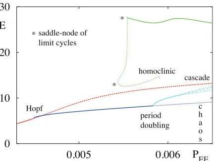
r/κcos(θ/2)independent ofαwith a non-zero fre-quency ω =αpr/κsin(θ/2). However, in general a Hopf bifurcation will depend on the relative time-scales in the model and should be determined as the solution ofdetE(iω) = 0. In practice it is much easier to numerically determine the stability of fixed points of the full ten dimensional model, defined by equa-tions (1–5), using software such as XPPAUT [29]. Moreover, this allows us to construct bifurcation dia-grams like those in Fig. 2, which shows the coexistence of a large and small amplitude periodic orbit, with time-course shown in Fig. 3. The large amplitude, (∼5

Hz) orbit has been suggested to correspond to a form of epileptic dynamics, whilst the smaller amplitude (∼10 Hz) oscillation is more consistent with the al-pha band of the EEG spectrum. Moreover, a period doubling cascade is supported and beyond this the model is known to support chaos. Indeed the chaotic behaviour has been extensively investigated in a se-ries of papers [31, 32, 30], highlighting that the route to chaos is actually via a novel Shilnikov saddle-node bifurcation. Note that in contrast the chaotic EEG pat-terns in the Freeman model of the olfactory system are generated via the Ruelle-Takens-Newhouse route [33]. For further discussion on the use of neural mass mod-els in epileptic modelling and human brain rhythms we refer the reader to [34, 35] and [36] respectively.

It is possible to recover a solely activity based model from the Liley model by treating the limit of fast re-laxation τa → 0. In this case the mean membrane

voltages are slaved to the dynamically evolving

con-0

10

20

30

0.005

0.006

E

EE

P

Hopf c

h a o s period

doubling

cascade saddle-node of

limit cycles

homoclinic *

* *

Figure 2: Bifurcation diagram for the Liley population model showing the absolute maximum ofEin terms ofPEEfor steady state (red), small amplitude periodic

(blue) and large amplitude periodic (green) orbits. Stable (unstable) branches are solid (dashed). Chaotic solutions are found after the period doubling cascade. Parameters are modified from [30] asPIE = 0.005763

ms−1_{, α}

EE =αIE = 1.01 ms−1, αII =αEI = 0.142

ms−1_{, W}

EE = WIE = 43.31, WII = WEI = 925.80,

βE= 0.3,βI= 0.27,θE= 21.0mV,θI= 29.0mVhE=

115.0mV,hI=−20.0mV with zero-delays∆ab= 0.

-15

0

30

0

500

1000

E

t (ms)

Figure 3: An example of multistability in the Liley population model. A small and large amplitude sta-ble rhythm co-exist over a range of parameter values. Here parameters are as in Fig. 2 withPEE = 0.006216

ductances and we may write E =E(gEE, gEI) and

I=I(gII, gIE). Symbolically the model now takes the

closed form

g=η∗[f+P], f =f({g}), (9)

where we suppress indices and use the notation{g}

to emphasise that the firing rate depends on the set of network conductances. A whole host of models can be described with such a system of equations, rang-ing from networks with many more than two mod-ules and a complicated dependence of the firing rate on the set of network conductances down to a single population with self-excitation. A very simple exam-ple of this latter case for a single conductanceg=ucan be obtained for the choice of an exponential synapse η(t) =αe−αt_{H(t)and assumingf=f(u)withP= 0,}

so that

1 + 1

α d dt

u=f(u). (10)

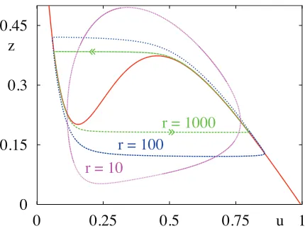
In some sense we may regard this model as one of the most basic to arise in mathematical neuroscience. Interestingly it has been subjected to modifications that improve its ability to model neuronal dynamics without recourse to abandoning the fast relaxation as-sumption. One of the main extensions of this type has been the inclusion of a term to describe refractoriness [2]. A particular example is that of Curtu and Ermen-trout [37]:

1

α du

dt =−u+

1− 1

R

Z t

t−R

u(s)ds

f(u), (11)

whereR is theabsolute refractory period of the neu-rons in the population. The fixed point u_ss satisfies the equation−uss+ (1−uss)f(uss) = 0. For a sigmoid

with0< f <1then there is at least one solution of this equation foru_ss∈(0,1/2). The characteristic equation determining the linear stability of the steady state is calculated asE(λ) = 0, with

E(λ) = λ

α+A+f(uss)

1−e−λR

λR , (12)

where A = 1−(1−u_ss)f0_(u

ss). This transcendental

equation allows for the possibility of complex roots, and not surprisingly it is possible to choose values for the slope and threshold of the sigmoid such that

0

0.15

0.3

0.45

0

0.25

0.5

0.75

u

1

z

r = 1000

r = 100

r = 10

Figure 4: Relaxation oscillations in an activity based single population with self-excitation and refractori-ness.r= 1000,T∼1.29.r= 100,T∼1.43.r= 10,T∼

2.24.β= 8,θ= 1/3. Thecubiccurve isz= 1−u/f(u).

a dynamic bifurcation defined byE(iω) = 0can occur [37]. Interestingly periodic solutions that emerge be-yond such a bifurcation can be analysed explicitly in some singular limit. To see this we write (11) as a two-dimensional delay differential equation:

u˙ =−u+ (1−z)f(u), (13)

˙

z=u(t)−u(t−1), (14)

where we have re-scaled time according tot 7→t/R and set= (αR)−1_{. Formally setting= 0 gives the}

processes whose combined effect is to modulate neu-ronal response. It is convenient to think of these pro-cesses in terms of local feedback mechanisms. For ex-ample, spike frequency adaptation (SFA) is a prop-erty of many single neurons and has been linked to the presence of a Ca2+ _{gated K}+ _current,I

AHP [39].

The generation of an action potential leads to a small calcium influx that incrementsIAHP, with the end

re-sult being a decrease in the firing rate response to per-sistent stimuli. A simple phenomenological model of this process is to add a current, that activates in the presence of high activity,I−gs, to the right hand side of (10) [40], where

τds

dt =−s+f(u), (15) andI is a constant bias. This form of SFA leads nat-urally to the emergence of periodic behaviour. In-deed in the limit of large τ (slow adaptation) and a for a steep sigmoid (largeβ) this period can be cal-culated explicitly asτlog((g−I)(1 +I)/(I(g−1−I))

forg >1 +Iand shows a classic relaxation oscillation betweenupanddownstates like those seen in biophys-ical models of slow (<1 Hz) oscillations [41]. An al-ternative approach, consistent with observations first made by Hill in 1936 [42], is to treat the threshold in the firing function to be state-dependent. This is ex-plored in detail in [43, 44] and shown to lead to exotic dynamics at the network level, including the emer-gence of dissipative solitons. However, rather than pursue these extensions in more detail we shall in-stead next show how to build tissue level models tak-ing as a starttak-ing point models of the form (9).

3

Tissue models

Here we will view a macroscopic part of the neocor-tex as being adequately modelled as a spatial assem-bly of population models – a neural field model. Such a viewpoint has already proven useful in understand-ing spatial aspects of the alpha rhythm and in partic-ular cortical travelling waves [6, 45]. For a recent per-spective on the use of neural field models in interpret-ing extrinsic optical imaginterpret-ing data (fromin vitro

exper-iments on pharmacologically treated brain slices) we refer the reader to [46].

To develop the extension of (9) to treat spatially con-tinuous neural sheets (such as a two-dimensional cor-tex) we will adopt thecontinuumassumption and treat a density of neurons at a point with inputs that arise from the delayed and weighted contribution of activ-ity at other points in the tissue. Because these interac-tions are mediated by long-range axonal fibres the re-sulting tissue-level model is inherently non-local and is often cast in the form of an integral equation. We represent this symbolically in the form

g=w⊗η∗f, (16)

where the operator⊗captures information about both anatomical connectivity patterns and the distribution of axonal delays. As a concrete example consider a set of two-dimensional interacting layered sheets (with both self and layer to layer interactions), each contain-ing only one cell type (either excitatory or inhibitory). The activity in layerainduced by that in layerb (gen-eralising equation (9)) then takes the form

uab=ηab∗ψab, (17)

whereψab=ψab(r, t)is given by Z

R2

dr0wab(r,r0)fb(r0, t− |r−r0|/vab) (18)

and fb is the firing rate in layerb. Herer∈R2 and wab(r,r0)prescribes the coupling strength between

po-sitionrin layeraand positionr0in layerb. The veloc-ity of an action potential travelling along a fibre con-necting layerb to layer ais denoted vab and

under-lies the space-dependent delay|r−r0|/vabfor signals

propagating over a distance|r−r0|. Note that (18) pro-vides meaning for the operator on the right hand side of the expressionψ=w⊗f. To close the system of equations one could choose the firing rate to depend on some dynamic mean-membrane potential as in the Liley model. Alternatively, to recover a purely activity based model in the spirit of Wilson-Cowan and Amari one could set fa =fa(ha), where ha =Pbuab. For

say that, apart from their relevance to neuroimaging, neural field models have found many applications in neuroscience, including to understanding the gener-ation of visual hallucingener-ations [48, 49], modelling ori-entation tuning in visual cortex area v1 [10], describ-ing travelldescrib-ing waves of activity in v1 durdescrib-ing binocular rivalry [50, 51], models of working memory [7] and encoding of continuous stimuli [52], motion percep-tion [8], somatosensory illusions [53], and developing a theory of cognitive robotics [54] for example.

Neural field models of the type (16) are nonlinear spatially extended systems and thus have all the nec-essary ingredients to support pattern formation. The analysis of such behaviour is typically performed with a mixture of linear Turing instability theory, weakly nonlinear perturbative analysis and numerical simu-lations (see [55] for a review). In the absence of de-tailed anatomical data it is common practice to con-sider cortico-cortical connectivity functions to be ho-mogeneous and isotropic so thatwab(r,r0) =wab(|r− r0|). In this case a homogeneous steady state is ex-pected and can be defined by hssa =

P

bWabfb(hssb),

whereWab=R_R2drwab(r). For concreteness we shall

take

wab(r) =w0abe−r/σab/(2π), (19)

where r= |r|. Linearising around the steady state and considering perturbations of the form ha(r, t)∼

eλt_eik·r_{, gives an equation for the continuous} spec-trumλ=λ(k), fork=|k|, in the formE(k, λ) = 0[56], whereE(k, λ) = det(D(k, λ)−I), and

[D(k, λ)]ab=η_eab(λ)Gab(k,−iλ)γb. (20)

Here γa =fa0(hssa)and Gab(k, ω)is the Fourier

trans-form ofGab(r, t) =wab(r)δ(t−r/vab)defined by

Gab(k, ω) = Z

R3

drdt Gab(r, t)e−i(k·r+ωt)

=w_ab0 Aab(ω)

(A2

ab(ω) +k2)3/2

, (21)

whereAab(ω) = 1/σab+iω/vab. Here we use a

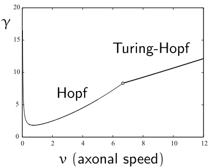
nota-tion that distinguishes funcnota-tions and their transforms simply by their arguments, namely(r, t)for the orig-inal space and (k, ω) for the Fourier space. An in-stability occurs when for the first time there are val-ues of k at which the real part ofλis non-negative.

0 5 10 15 20

0 2 4 6 8 10 12

γ

v

(

axonal speed

)

Hopf

Turing-Hopf

Figure 5: Critical curves showing the instability bor-ders for dynamic instabilities in the(v, γ)plane, where γ=f0(hss_).

A Turing bifurcation point is defined as the smallest value of some order parameter for which there ex-ists some non-zerokc satisfying Re (λ(|kc|)) = 0. It is said to be staticif Im (λ(|kc|)) = 0 and dynamic if Im(λ(|kc|))≡ωc6= 0. The dynamic instability is often

referred to as a Turing-Hopf bifurcation and generates a global pattern with wavenumber|kc|, which moves coherently with a speedc=ωc/|kc|, i.e. as a periodic

travelling wave train. If the maximum of the disper-sion curve is at|kc|= 0then the mode that is first ex-cited is another spatially uniform state. Ifωc 6= 0, we

would then expect the emergence of a coherent net-work oscillation with frequencyωc.

For example, consider two populations, one exci-tatory and one inhibitory with a common firing rate functionfa=f and single axonal conduction velocity

vab=v, and use the labelsa∈ {E, I}, withwEE,IE0 = 1,

w0

II,EI =−4, αab = 1and∆ba= 0. In neocortex the

extent of excitatory connectionsWaE is broader than

that of inhibitory connections WaI, and so we take

σaI = 1andσaE = 2. In Fig. 5 we show a plot of the

critical curves in the(v, γ)plane above which the ho-mogeneous steady state,hss

E,I =hss, is unstable to

dy-namic instabilities with|kc|= 0(bulk oscillations) and

1.98 1.985 1.99 1.995 2 2.005 2.01 2.015 2.02

Figure 6: Snapshots of a periodic travelling wave in uEE, each1/4of a period later than the previous one

(ordered top left, top right, bottom left, bottom tight), for the 2D model of Fig. 5 atv= 12andγ= 15(on a

30×30domain).

bifurcation.

Despite the natural framework for neural field models being non-local integral equations with space-dependent delays the techniques for analysing them are nowhere near as developed as they are for local PDE models. Thus for this reason it is sometimes worth constructing equivalent PDE models. To date progress in this area has been made by Nunez [6] and Jirsa and Haken [19] for neural field models in one spatial dimension with axonal delays, making links to the theory of damped inhomogeneous wave equa-tions. For example in a one-dimensional setting with wab(x) =e−|x|/σab/(2σab), the equivalent PDE model

toψ=w⊗fis

A2

ab−∂xxψab=

1

σab

Aabfb, (22)

where

Aab=

₁

σab

+ 1

vab

∂t

. (23)

Equation (22) is the Jirsa-Haken-Nunez brain wave equation [19, 6, 57]. Turing instabilities in such mod-els (built from two populations) have been exhaus-tively analysed in [58, 59] and lead to bifurcation sce-narios consistent with those in Fig. 5, when consider-ing analogous architectures. Moreover, a weakly

non-linear analysis of the travelling and standing waves that develop beyond the point of instability has been developed. The appropriate amplitude equations are found to be the coupled mean-field Ginzburg-Landau equations describing a Turing-Hopf bifurcation with modulation group velocity ofO(1). In particular this has allowed an investigation of Benjamin-Feir mod-ulational instabilities in which a periodic travelling wave (of moderate amplitude) loses energy to a small perturbation of other waves with nearly the same fre-quency and direction. For asymmetric kernels (w(x)6=

w(−x)) or symmetric kernels with a peak away from the origin then the stability analysis of the homoge-neous steady state involves the solution of transcen-dental equations (as it would for an ordinary differen-tial equations with a fixed delay), though can be anal-ysed making use of Lambert functions [60].

For a single self-coupled population withσaa=σ,

vaa=vand a simple exponential synaptic filterηaa=

αe−αt_{H(t), (22) also supports travelling fronts [61].}

Moreover, for steep sigmoids (β → ∞andθa=θ) the

speed can be calculated in closed form as

c= (2θ−1)v

2θ−1−2θv/(ασ). (24)

This strong dependence of the wave speed on the threshold θ has now been indirectly established in rat cortical slices (bathed in the GABAA blocker

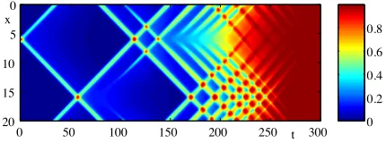
pi-crotoxin) [62]. An applied positive (negative) electric field across the slice increased (decreased) the speed of wave propagation, consistent with (24) assuming that a positive (negative) electric field reduces (increases) the thresholdθ. Of course travelling waves are also possible solutions of the more general non-local for-malism described by (16), and have been explored mathematically in a number of papers, reviewed in [11], with a particular regard to studying waves in cor-tical slices [63], and notably epileptiform activity [64].

pur-t

0 50 100 150 200 250 300

0

5

10

15

20 0

0.2 0.4 0.6 0.8 x

Figure 7: Numerical simulations of a coupled neural field model in one spatial dimension showing the in-teraction of two travelling pulses and the emergence of transient complex behaviour ultimately leading to an elevated firing rate across the whole tissue. The model is defined by[A2

a−∂xx]ψa= ΓaAaH(ue−ui−

θ)/σa,Aa = (σa−1+va−1∂t),(1 +α−a1∂t)ua =ψa, with

a∈ {e, i}, describing a model with short range inhi-bition and long range excitation. The plot shows the evolution of ue with ve= 0.2, vi = 1, αe =αi = 1,

Γe= 1,Γi= 0.7,σe= 2,σi= 1andθ= 0.07.

sued for waves in one space-dimension using a stan-dard travelling wave analysis (in which one looks for stationary profiles in a co-moving frameξ=x−ctof speedc < v). This can often only be done numerically, say using the techniques of spatial dynamics and con-structing homoclinic connections, as in [61]. Interest-ingly propagating pulses of (22) can scatter in novel ways, leading to an elevated firing across the whole tissue [65]. An example of this is shown in Fig. 7.

Finding equivalent brain wave equations in two-spatial dimensions has proved far more challenging [18], with various approximations being made to ob-tain a local model. The most common of these is the so-called long-wavelength approximation, although this has recently been improved upon in [56]. In the former case this amounts to expanding (21) around k = 0 for small k, yielding a “nice” rational poly-nomial structure to give(A2_ab(ω) + 3k2/2)ψab(k, ω) =

fb(k, ω) which may then be inverse transformed to

give the telegraph PDE:

A2

ab−

3 2∇

2

ψab=w0abfb. (25)

This model has been intensively studied by a number of authors in the context of EEG modelling, see for ex-ample [66, 67, 68].

Undoubtedly the assumption of isotropic connec-tivity is a strong one for the modelling of cortical tis-sue. That it has been pursued so aggressively to date is more a reflection of the mathematical tractability of such models as opposed to their relation to real tis-sue. Indeed questions about the existence, unique-ness and absolute stability of solutions for truly in-homogeneous models are only just beginning to be addressed using tools from functional analysis [69]. However, one symmetry breaking effect that can be tackled without too much effort is that of the loss of continuous rotation symmetry. This is an important issue to treat in light of the fact that it is now known that (visual) cortex has a crystalline micro-structure at the millimeter length scale (reviewed in [70]). This has given rise to the notion ofpatchyconnections that break continuous rotation symmetry (but not neces-sarily continuous translation symmetry). The natural way to model this is to introduce a modified connec-tivity kernelwP_ab(r,r0)as

wP_ab(r,r0) =wab(|r−r0|)Jab(r−r0), (26)

whereJab(r)varies periodically with respect to a

reg-ular planar latticeL. Note that the patchy kernelwP ab

is homogeneous, but not isotropic. The generalisation of brain wave equations to treat patchiness that arise via periodic modulation of an isotropic kernel has re-cently been developed by Robinson [71] and analysed further in [56]. In essence the brain wave equation (25) is replaced by an infinite set of PDEs – indexed by the reciprocal lattice vectorsqof the underlying latticeL, that arise in the Fourier series representation

Jab(r) = X

q

J_abqeiq·r. (27)

In the long-wavelength approximation this set of PDEs is obtained from (25) under the replacement

∇ → ∇ −iq, ψab→ψqab and uab→ηab∗P_qJabqψ

q

ab.

compared to the unmodulated case shown in Fig. 5, the Hopf bifurcation is transformed to a Turing-Hopf bifurcation with critical wavevectors coinciding with those of the lattice. With increasingvthe dominant bi-furcation is also of Turing-Hopf type. However, in this case it is a ring of wavevectors surrounding the recip-rocal lattice vectors that go unstable first. In both cases this suggests the emergence of periodic travelling waves aligned to the lattice size and direction, which are indeed observed in direct numerical simulations [56]. For a more general inhomogeneous kernel of the formwI

ab(r,r 0_{) =w}

ab(|r−r0|)Jab(r0), then the PDE

formulation goes over with the source term fb(r, t)

in (25) replaced byJab(r)fb(r, t). When the

modulat-ing kernel Jab(r) varies both weakly and rapidly in

space then one may use techniques from homogeni-sation theory to study wave propagation and its fail-ure [72]. Indeed recent work avoiding the assumption of rapid spatial variation shows that for a one dimen-sional neural field model withJ(x) = 1 +sin(2πx/σ)

andf(u) =H(u−θ)then pulsating waves can occur (where say a front edge is modulated in space) with a wave speedc0

p

1−(/c)2so that propagation

fail-ure occurs for some > c =c(σ, θ)[73]. Herec0 is

the speed of the wave in the homogeneous case (when = 0and see equation (24) for example). Further treat-ment of heterogeneous connection topologies can be found in [74, 75, 76, 77].

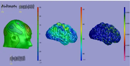
One of the more recent and compelling uses of neu-ral field modelling is by Bojak and colleagues [13, 14]. They relate different (co-registered) imaging modal-ities to one another, namely EEG (with its excellent temporal resolution) and fMRI (with its superior spa-tial resolution) by modelling an underlying neural generator that is based upon the Liley model [18] dis-cussed earlier. Importantly regional connectivity data is incorporated using the CoCoMac database [78], which contains information on structural connectiv-ity in the macaque brain (from tract-tracing experi-ments). In order to be compatible with true fMRI im-ages their computational model uses triangular spa-tial grids matched to cortical geometries extracted from structural MR images. From the activity of the

Figure 8: An EEG scalp isopotential (left) generated from the mean membrane excitatory potential of a neural field model (middle) and the corresponding fMRI BOLD signal construction on the cortical surface (right), illustrating the capabilities of the recent com-putational framework developed by Bojak and col-leagues [13, 14]. Associated animations may be found at http://www.mbfys.ru.nl/neuropi/cns09/.

model cortical sheet, the simulated EEG at the scalp is found using a realistic volume conductor model. The response for fMRI BOLD is constructed using an es-tablished model for neurovascular coupling and con-volving with “Balloon-Windkessel” haemodynamics [79]. This is one of the first attempts to seriously com-bine neuronal dynamics and brain connectivity along the lines advocated in [80]. An example of output from their modelling approach is shown in Fig. 8. For a recent review on the challenges in combining EEG and fMRI imaging modalities using neural models we refer the reader to Valdes-Sosaet al. [81], and for work on folded three-dimensional cortical sheets and their use in forward EEG and MEG prediction see Jirsaet al. [82]. Other work on using realistic anatomical con-nectivities in large scale neural models (especially as it relates to the resting brain state) can be found in [83, 84, 85].

gener-alise such models even further to treat feature selec-tivity such as that observed in visual cortex for ori-entation [10], spatial frequency [91] and texture [92]. In this case neural activity is now also considered to be a function of some set of featuresχ and interac-tions must be specified by a feature dependent kernel wab(r0, t0, χ0|r, t, χ). Indeed with the increasing march

of experimental progress in recording from popula-tions of neurons we are now ideally poised to push forward with the development of multi-scale models that can integrate macroscopic models at large spa-tial scales with models at the microscopic scale [93]. One outstanding challenge for the development of tis-sue level firing rate models is how best to include gap junction coupling [94].

4

Discussion

A known limitation of neural field models is that they only try to track mean activity levels and can-not, by definition, track the higher order correlations of any underlying spiking model. Of course one approach would be to abandon them altogether in favour of more biophysically detailed models. How-ever, as we have discussed here they can go a re-markably long way to providing a framework for interpreting neuro-imaging data whilst maintaining contact with known brain structure, dynamics and function. Rather it is preferable to work with spik-ing models and establish more concretely the link to mean activity models, and when more sophisticated kinetic models of brain activity are required [95, 96]. Moreover, in some instances it is possible to analyse spiking networks directly (usually under the assump-tion of global coupling and fast synaptic interacassump-tions) as in the spike-density approach [97, 98, 99], which makes heavy use of the numerical solution of cou-pled partial differential-integral equations. In other situations equations going beyond the mean-field ap-proach have been proposed that govern second-order correlations [100, 101, 102, 103]. Indeed there has been a recent upsurge of interest in this area adapting methods from non-equilibrium statistical physics to

determine corrections to mean-field theory involving equations for two-point and higher-order cumulants [104, 105]. One immediate, yet potentially tractable, challenge would be to develop a framework for un-derstanding networks of synaptically interacting non-linear integrate-and-fire networks. At the single neu-ron level such models are already known to be able to capture many different physiological firing pat-terns and at the network level are computationally far cheaper to implement than their conductance based cousins yet still able to generate the rich repertoire of behaviour seen in a real nervous system [106]. One step in this direction has already been undertaken for the absolute-integrate-and-fire model [107] and this may well be a natural spiking model to pursue for the development of a specific soluble spiking neuro-dynamics.

Acknowledgements

SC would like to thank Carlo Laing and David Liley for many interesting discussions concerning the mod-elling of cortical tissue and Ingo Bojak for providing Fig. 8.

References

[1] H Markram. The blue brain project. Nature Reviews

Neuroscience, 7:153–160, 2006.

[2] H R Wilson and J D Cowan. Excitatory and inhibitory

interactions in localized populations of model

neu-rons. Biophysical Journal, 12:1–24, 1972.

[3] H R Wilson and J D Cowan. A mathematical theory of the functional dynamics of cortical and thalamic

ner-vous tissue.Kybernetik, 13:55–80, 1973.

[4] S Amari. Homogeneous nets of neuron-like elements.

Biological Cybernetics, 17:211–220, 1975.

[5] S Amari. Dynamics of pattern formation in

lateral-inhibition type neural fields. Biological Cybernetics,

27:77–87, 1977.

[7] C R Laing, W C Troy, B Gutkin, and G B Ermen-trout. Multiple bumps in a neuronal model of

work-ing memory. SIAM Journal on Applied Mathematics,

63:62–97, 2002.

[8] M A Geise. Neural Field Theory for Motion Perception.

Kluwer Academic Publishers, 1999.

[9] K Zhang. Representation of spatial orientation by the intrinsic dynamics of the head-direction cell

ensem-ble: A theory. Journal of Neuroscience, 16:2112–2126,

1996.

[10] R Ben-Yishai, L Bar-Or, and H Sompolinsky. Theory of

orientation tuning in visual cortex. Proceedings of the

National Academy of Sciences USA, 92:3844–3848, 1995.

[11] S Coombes. Waves, bumps, and patterns in neural

field theories.Biological Cybernetics, 93:91–108, 2005.

[12] S Coombes. Neural fields. Scholarpedia:

http://www.scholarpedia.org /article/Neural fields, 1:1373, 2006.

[13] I Bojak, T F Oostendorp, A T Reid, and R K ¨otter.

Re-alistic mean field forward predictions for the

integra-tion of co-registered EEG/fMRI. BMC Neuroscience,

10:L2, 2009.

[14] T F Oostendorp, I Bojak, A T Reid, and R K ¨otter.

Con-necting mean field models of neural activity to EEG

and fMRI data.Brain Topography, to appear, 2009.

[15] P beim Graben and R Potthast. Inverse problems in

dynamic cognitive modeling.Chaos, 19:015103, 2009.

[16] K E Stephan, L M Harrison, S J Kiebel, O David, W D Penny, and K J Friston. Dynamic causal models of neural system dynamics: current state and future

ex-tensions.Journal of Biosciences, 32:129–144, 2007.

[17] J Daunizeau, S J Kiebel, and K J Friston. Dynamic causal modelling of distributed electromagnetic

re-sponses.NeuroImage, 47:590–601, 2009.

[18] D T J Liley, P J Cadusch, and M P Dafilis. A spatially

continuous mean field theory of electrocortical activ-ity.Network, 13:67–113, 2002.

[19] V K Jirsa and H Haken. A derivation of a macroscopic

field theory of the brain from the quasi-microscopic

neural dynamics.Physica D, 99:503–526, 1997.

[20] B H Jansen and V G Rit. Electroencephalogram and visual evoked potential generation in a mathematical

model of coupled cortical columns. Biological

Cyber-netics, 73:357–366, 1995.

[21] F H Lopes da Silva, A Hoeks, and L H Zetterberg.

Model of brain rhythmic activity.Kybernetik, 15:27–37,

1974.

[22] O David and K J Friston. A neural mass model for

MEG/EEG: coupling and neuronal dynamics.

Neu-roImage, 20:1743–1755, 2003.

[23] F Grimbert and O Faugeras. Bifurcation analysis

of Jansen’s neural mass model. Neural Computation,

18:3052–3068, 2006.

[24] R A Stefanescu and V K Jirsa. A low dimensional

description of globally coupled heterogeneous neural

networks of excitatory and inhibitory neurons. PLoS

Compututational Biology, 4:e1000219, 2008.

[25] C R Laing. On the application of “equation-free

mod-elling” to neural systems. Journal of Computational

Neuroscience, 20:5–23, 2006.

[26] C R Laing and I G Kevrekidis. Periodically-forced fi-nite networks of heterogeneous coupled oscillators: a

low-dimensional approach. Physica D, 237:207–215,

2008.

[27] S Coombes and C Laing. Delays in activity-based

neu-ral networks. Philosophical Transactions of the Royal

So-ciety A, 367:1117–1129, 2009.

[28] M Breakspear, J A Roberts, J R Terry, S Rodrigues,

N Mahant, and P A Robinson. A unifying explana-tion of primary generalized seizures through

nonlin-ear brain modeling and bifurcation analysis. Cerebral

Cortex, 16:1296–1313, 2006.

[29] B Ermentrout. Simulating, Analyzing, and Animating

Dynamical Systems: A Guide to XPPAUT for Researchers and Students. Society for Industrial & Applied

Mathe-matics, 2002.

[30] M P Dafilis, F Frascoli, P J Cadusch, and D T J

Liley. Chaos and generalised multistability in a

meso-scopic model of the electroencephalogram. Physica D,

238:1056–1060, 2009.

[31] M P Dafilis, D T J Liley, and P J Cadusch. Robust chaos

in a model of the electroencephalogram: Implications

for brain dynamics.Chaos, 11:474–478, 2001.

[32] L van Veen and D T J Liley. Chaos via Shilnikov’s saddle-node bifurcation in a theory of the

electroen-cephalogram.Physical Review Letters, 97:208101, 2006.

[33] W J Freeman. Simulation of chaotic EEG patterns with

a dynamic model of the olfactory system. Biological

[34] J Milton and P Jung, editors. Epilepsy as a Dynamic Disease. Springer, 2003.

[35] B Schelter and J Timmer, editors. Seizure Prediction

in Epilepsy: From Basic Mechanisms to Clinical

Applica-tions. Wiley-VCH, 2008.

[36] D A Steyn-Ross and M Steyn-Ross, editors. Modeling

Phase Transitions in the Brain, volume 4 ofSpringer Se-ries in Computational Neuroscience. Springer, 2010.

[37] R Curtu and B Ermentrout. Oscillations in a refractory

neural net. Journal of Mathematical Biology, 43:81–100,

2001.

[38] R Fitzhugh. Impulses and physiological states in

the-oretical models of nerve membranes.Biophysical

Jour-nal, 1182:445–466, 1961.

[39] Y H Liu and X J Wang. Spike-frequency adaptation of a generalized leaky integrate-and-fire model

neu-ron. Journal of Computational Neuroscience, pages 25– 45, 2001.

[40] C van Vreeswijk and D Hansel. Patterns of synchrony

in neural networks with spike adaptation. Neural

Computation, Jan 2001.

[41] A Compte, M V Sanchez-Vives, D A McCormick, and X-J Wang. Cellular and network mechanisms of slow

oscillatory activity (<1Hz) and wave propagation in

a cortical network model. Journal of Neurophysiology,

89:2707–2725, 2003.

[42] A V Hill. Excitation and accommodation in nerve.

Proceedings of the Royal Society of London. Series B, Bi-ological Sciences, 119:305–355, 1936.

[43] S Coombes and M R Owen. Bumps, breathers,

and waves in a neural network with spike frequency

adaptation.Physical Review Letters, 94(148102), 2005.

[44] S Coombes and M R Owen. Exotic dynamics in a fir-ing rate model of neural tissue with threshold

accom-modation. AMS Contemporary Mathematics, ”Fluids

and Waves: Recent Trends in Applied Analysis”, 440:123– 144, 2007.

[45] A van Rotterdam, F H Lopes da Silva, J van den Ende,

M A Viergever, and A J Hermans. A model of the spatial-temporal characteristics of the alpha rhythm.

Bulletin of Mathematical Biology, 44:283–305, 1982.

[46] F Grimbert. Mesoscopic models of

cor-tical structures. PhD thesis, University

of Nice-Sophia Antipolis,

http://www-sop.inria.fr/members/Francois.Grimbert/ docs/thesis revised.pdf.zip, 2008.

[47] A Destexhe and T J Sejnowski. The Wilson-Cowan

model, 36 years later. Biological Cybernetics, 101:1–2,

2009.

[48] G B Ermentrout and J D Cowan. A mathematical

the-ory of visual hallucination patterns. Biological

Cyber-netics, 34:137–150, 1979.

[49] P C Bressloff, J D Cowan, M Golubitsky, P J Thomas, and M Wiener. Geometric visual hallucinations, Eu-clidean symmetry and the functional architecture of

striate cortex.Philosophical Transactions of the Royal

So-ciety London B, 40:299–330, 2001.

[50] H R Wilson, R Blake, and S-H Lee. Dynamics of

travel-ling waves in visual perception. Nature, 412:907–910,

2001.

[51] S-H Lee, R Blake, and D J Heeger. Travelling waves of activity in primary visual cortex during binocular

rivalry.Nature Neuroscience, 8:22–23, 2005.

[52] S Wu, K Hamaguchi, and S Amari. Dynamics and

computation of continuous attractors. Neural

Compu-tation, 20:994–1025, 2008.

[53] H G E Meijer, J Trojan, D Kleinb ¨ohl, R H ¨olz, and J R Buitenweg. A dynamic neural model of localization

of brief successive stimuli in saltation. BMC

Neuro-science, 10:P350, 2009.

[54] W Erlhagen and E Bicho. The dynamic neural field

approach to cognitive robotics. Journal of Neural

Engi-neering, 3:R36–R54, 2006.

[55] P C Bressloff. Les Houches Lectures in Neurophysics,

chapter Pattern formation in visual cortex.

Springer-Verlag, 2004.

[56] S Coombes, N A Venkov, L Shiau, I Bojak, D T J Liley, and C R Laing. Modeling electrocortical activ-ity through improved local approximations of integral

neural field equations. Physical Review E, 76:051901,

2007.

[57] P l Nunez. Neocortical Dynamics and Human EEG

Rhythms. Oxford University Press, 1995.

[58] N A Venkov, S Coombes, and P C Matthews. Dy-namic instabilities in scalar neural field equations

with space-dependent delays. Physica D, 232:1–15,

2007.

[59] N A Venkov. Dynamics of Neural Field

Models. PhD thesis, School of

Mathemat-ical Sciences, University of Nottingham,

[60] P Grindrod and D Pinotsis. On the spectra of certain integro-differential-delay problems with applications

in neurodynamics.Physica D, submitted, 2009.

[61] S Coombes, G J Lord, and M R Owen. Waves

and bumps in neuronal networks with axo-dendritic

synaptic interactions.Physica D, 178:219–241, 2003.

[62] K A Richardson, S J Schiff, and B J Gluckman. Control

of traveling waves in the mammalian cortex.Physical

Review Letters, 94:028103, 2005.

[63] J-Y Wu, X Huang, and C Zhang. Propagating Waves of Activity in the Neocortex: What They Are, What

They Do.The Neuroscientist, 14(5):487–502, 2008.

[64] D J Pinto and G B Ermentrout. Spatially structured activity in synaptically coupled neuronal networks: I.

Travelling fronts and pulses.SIAM Journal on Applied

Mathematics, 62:206–225, 2001.

[65] C Laing and S Coombes. The importance of differ-ent timings of excitatory and inhibitory pathways in

neural field models. Network: Computation in Neural

Systems, 17:151 – 172, 2006.

[66] M L Steyn-Ross, D A Steyn-Ross, J W Sleigh, and

D T J Liley. Theoretical electroencephalogram sta-tionary spectrum for a white-noise-driven cortex: Ev-idence for a general anesthetic-induced phase

transi-tion.Physical Review E, 60:7299–7311, 1999.

[67] P A Robinson, C J Rennie, J J Wright, H Bahramali,

E Gordon, and D l Rowe. Prediction of

electroen-cephalographic spectra from neurophysiology.

Physi-cal Review E, 63:021903, 2001.

[68] I Bojak and D T J Liley. Modeling the effects of

anes-thesia on the electroencephalogram. Physical Review

E, 71:041902, 2005.

[69] O Faugeras, F Grimbert, and J-J Slotine. Absolute

sta-bility and complete synchronization in a class of

neu-ral fields models. SIAM Journal on Applied

Mathemat-ics, 69:205–250, 2008.

[70] P C Bressloff and J D Cowan. The visual cortex as a

crystal.Physica D, 173:226–258, 2002.

[71] P A Robinson. Patchy propagator, brain dynamics, and the generation of spatially structured gamma

os-cillations.Physical Review E, 73:041904, 2006.

[72] P C Bressloff. Traveling fronts and wave propagation

failure in an inhomogeneous neural network.Physica

D, 155, 2001.

[73] S Coombes and C R Laing. Neural fields with periodic

modulation.Physical Review E, in preparation, 2009.

[74] V K Jirsa and J A S Kelso. Spatiotemporal pattern for-mation in neural systems with heterogeneous

connec-tion topologies.Physical Review E, 62:8462–8465, 2000.

[75] P C Bressloff. Spatially periodic modulation of cortical

patterns by long-range horizontal connections.

Phys-ica D, 185:131–157, 2003.

[76] H Schmidt, A Hutt, and L Schimansky-Geier. Wave

fronts in inhomogeneous neural field models.Physica

D, 238:1101–1112, 2009.

[77] C A Brackley and M S Turner. Two-point

heteroge-neous connections in a continuum neural field model.

Biological Cybernetics, 100:371–383, 2009.

[78] R K ¨otter and E Wanke. Mapping brains without

co-ordinates.Philosophical Transactions of the Royal Society

B, 360:751–766, 2005.

[79] K J Friston, L Harrison, and W Penny. Dynamic causal

modelling. NeuroImage, 19:1273–1302, 2003.

[80] M Breakspear and V K Jirsa. Neuronal dynamics and

brain connectivity. In V K Jirsa and A R McIntosh,

editors, Handbook of Brain Connectivity, pages 3–64.

Springer, 2007.

[81] P A Valdes-Sosa, J M Sanchez-Bornot, R C Sotero,

Y Iturria-Medina, Y Aleman-Gomez Y, J

Bosch-Bayard, F Carbonell, and T Ozaki. Model driven

EEG/fMRI fusion of brain oscillations. Human Brain

Mapping, 30:2701–2721, 2009.

[82] V K Viktor Jirsa, K J Jantzen, A Fuchs, and J A Scott

Kelso.Information Processing in Medical Imaging,

chap-ter Neural Field Dynamics on the Folded Three-Dimensional Cortical Sheet and Its Forward EEG and MEG, pages 286–299. Springer Berlin, 2001.

[83] C J Honey, R K ¨otter, M Breakspear, and O Sporns.

Network structure of cerebral cortex shapes

func-tional connectivity on multiple time scales.

Proceed-ings of the National Acadamy of Sciences USA National

Academy of Sciences, USA, 104:10240–10245, 2007.

[84] A Ghosh, Y Rho, A R McIntosh, R K ¨otter, and V K Jirsa. Noise during rest enables the exploration of the

brain’s dynamic repertoire. PLoS Computational

Biol-ogy, 4(10):e1000196, 2008.

[85] G Deco, V K Jirsa, A R McIntosh, O Sporns, and R K ¨otter. Key role of coupling, delay, and noise in

resting brain fluctuations. Proceedings of the National

[86] S Coombes. Dynamics of synaptically coupled

integrate-and-fire-or-burst neurons.Physical Review E,

67:041910, 2003.

[87] Z P Kilpatrick and P C Bressloff. Effects of synaptic depression and adaptation on spatiotemporal

dynam-ics of an excitatory neuronal network. Physica D, to

appear, 2009.

[88] M Zachariou, D W N Dissanayake, S Coombes, M R Owen, and R Mason. Sensory gating and its

modula-tion by cannabinoids: electrophysiological,

computa-tional and mathematical analysis. Cognitive

Neurody-namics, pages 159–170, 2008.

[89] D T J Liley, P J Cadusch, M Gray, and P J Nathan. Drug induced modification of the system properties asso-ciated with spontaneous electroencephalographic

ac-tivity.Physical Review E, 68:051096, 2003.

[90] B L Foster, I Bojak, and D T J Liley. Population based models of cortical drug response: insights from

anaes-thesia.Cognitive Neurodynamics, 2:283–296, 2008.

[91] P C Bressloff and J D Cowan. Spherical model of ori-entation and spatial frequency tuning in a cortical

hy-percolumn.Philosophical Transactions of the Royal

Soci-ety B, 358:1643–1667, 2003.

[92] P Chossat and O Faugeras. Hyperbolic planforms

in relation to visual edges and textures perception.

http://arxiv.org/abs/0907.0963v2, 2009.

[93] O Faugeras, J Toubal, and B Cessac. A constructive

mean-field analysis of multi population neural net-works with random synaptic weights and stochastic

inputs.Frontiers in Computational Neuroscience, 3, 2009.

[94] S Coombes. Neuronal networks with gap junctions: A study of piece-wise linear planar neuron models.

SIAM Journal on Applied Dynamical Systems, 7:1101–

1129, 2008.

[95] M Breakspear and S Knock. Kinetic models of brain

activity.Brain Imaging and Behavior, 2:270–288, 2008.

[96] G Deco, V K Jirsa, P A Robinson, M Breakspear, and K J Friston. The dynamic brain: From spiking neurons

to neural masses and cortical fields. PLoS

Compututa-tional Biology, 4:e1000092, 2008.

[97] D Q Nykamp and D Tranchina. A population density approach that facilitates large-scale modeling of

neu-ral networks: Extension to slow inhibitory synapses.

Neural Computation, 13:511–546, 2001.

[98] D Cai, L Tao, M Shelley, and D W McLaughlin. An effective kinetic representation of fluctuation-driven neuronal networks with application to simple and

complex cells in visual cortex. Proceedings of the

Na-tional Academy of Sciences of the United States of America, 101:7757–7762, 2004.

[99] F Apfaltrer, C Ly, and D Tranchina. Population

density methods for stochastic neurons with realistic

synaptic kinetics: Firing rate dynamics and fast

com-putational methods. Network: Computation in Neural

Systems, 17:373 – 418, 2006.

[100] I Ginzburg and H Sompolinsky. Theory of

correla-tions in stochastic neural networks.Physical Review E,

50:3171–3191, 1994.

[101] H Soula and C C Chow. Stochastic dynamics of a

finite-size spiking neural network. Neural

Computa-tion, 19:3262–3292, 2007.

[102] S E Boustani and A Destexhe. A master equation for-malism for macroscopic modeling of asynchronous

ir-regular activity states. Neural Computation, 21:46–100,

2009.

[103] B Kriener, T Tetzlaff, A Aertsen, M Diesmann, and

S Rotter. Correlations and population dynamics in

cortical networks. Neural Computation, 20:2185–2226,

2008. PMID: 18439141.

[104] M A Buice, J D Cowan, and C C Chow.

System-atic fluctuation expansion for neural network activity

equations. Neural Computation, to appear, 2009.

[105] P C Bressloff. Stochastic neural field theory and the

system-size expansion.SIAM Journal on Applied

Math-ematics, submitted, 2009.

[106] E M Izhikevich and G M Edelman. Large-scale model

of mammalian thalamocortical systems.Proceedings of

the National Academy of Sciences, 105:3593–3598, 2008.

[107] S Coombes and M Zachariou. Coherent Behavior in

Neuronal Networks, chapter Gap junctions and