Statistical bias in isotope ratios

Statistical bias in isotope ratios

Christopher D. Coath

⇤a

_{, Robert C. J. Steele}

a‡

_{and W. Fred Lunnon}

b

Received Xth XXXXXXXXXX 20XX, Accepted Xth XXXXXXXXX 20XX First published on the web Xth XXXXXXXXXX 200X

DOI: 10.1039/b000000x

This paper presents the mathematics of the systematic bias in the expected value of the ratio of two noise-corrected Poisson-distributed variables, such as ion counting measurements. Such bias can lead to the reporting of incorrect ratios and, in some cases, systematic correlations with other measurements which can impact the scientific interpretation. We describe a novel method of treating such measurements which results in a negligible, exponentially-small bias. We also re-examine the conven-tional approach deriving an exact expression for the bias including the noise correction explicitly.

1 Introduction

Analysts measuring a time series of ion beam intensities are faced with choices of how to process the data in order to esti-mate intensity ratios. Is it preferable, for example, to calculate the mean of the ratios, the ratio of the means or is there a bet-ter approach entirely? At the heart of the problem is the fact that the mean value a ratio estimator returns, over the long term, is biasedrelative to the true ratio being estimated. A simple example serves to illustrate the phenomenon of bias as follows. Suppose we write a 1 and a 3 on the faces of coin A and a 3 and 5 on the faces of coin B. Clearly, the mean value of a coin flip is 2 and 4 for coins A and B respectively. We now flip the two coins and record the ratio,B/A, as indicated by the upturned faces. In such an experiment, there are four equally probable outcomes: 3/1, 3/3, 5/1, and 5/3. Hence, the

expectation valueof the ratio,E(B/A) = (3+1+5+5/3)/4 or 8/3. The expectation value of B/A is the mean value of

B/Aover the long term. If we had hoped to estimate the ‘true’ ratio equal to the ratio of the means for each coin, 4/2=2, then clearly the estimatorB/Ais biased. We define the bias as the relative difference betweenE(B/A)and the true ratio. In this example, therefore, the bias is(8/3 2)/2=1/3.

The situation with ratios of ion-counting signals in isotope ratio measurements is directly analogous. The number of ions counted is accurately modelled by Poisson statistics which states that the probability of detectingXions is given by

Pois(X;µx) =e µxµxX/X!, (1)

a _{University of Bristol, School of Earth Sciences, Wills Memorial Building,} Queens Rd., Bristol, U.K. Fax: +44 (0)117 925 3385; Tel: +44 (0)117 954 5370; E-mail: [email protected]

b _{Department of Computer Science, National University of Ireland,} Maynooth, co. Kildare, Republic of Ireland.

‡ _{Present address: University of California, Los Angeles, Department of}

Earth and Space Sciences, 595 Charles Young Dr. E., Los Angeles, CA 90095-1567, U.S.A.

whereµx is thepopulation mean or expectation value of X.

Note that this single parameter,µx, characterises the Poisson

distribution. An analyst may wish to calculate an estimate of µx/µy, the ratio of the expectation values of two such signals,

X andY. More generally, it is often the case that analyte sig-nals are superposed on ‘noise’, whose origin may be in the detector (darknoise), spectral or contamination during sample preparation. Regardless of origin the mean noise is often as-sumed to be constant, is determined empirically and the mea-sured signals corrected for its contribution. Let the mean noise contribution toXandY beµx0andµy0respectively. The ratio

to be estimated,R, is, therefore, given by

R=µ_µx µx0

y µy0. (2)

In principal, any function, f(X,Y), may have it’s bias rela-tive toRdetermined by deriving the expectation valve,E(f), given by the double summation over allX andY of f(X,Y)·

Pois(X;µx)·Pois(Y;µy). For example, the commonly-used

ra-tio estimator,

r0=X_{Y µ}µx0

y0, (3)

is considered in section 2 but, even without detailed analysis,

r0is clearly problematic for any integer value ofµy0, including

zero, asE(r0)does not exist due to the non-zero probability

of events where the denominator,Y µy0, is zero. In section 3

a novel,quasi-unbiased ratio estimator is proposed, which is well behaved for allYandµy0.

1.1 Previous work

Coakleyet al.1_{and Oglioreet al.}2_{have shown thatX/Y is a}

biasedestimate ofR. Similar approaches by both1,2_yield

in the limit of largeµy. As we shall show in section 2, this

ap-proximation holds providingY =0 events are excluded from the distribution. Noise correction is not considered explicitly but, since the method used by these authors is rather general, it is straightforward to include it as a modification of the dis-tribution. Note that equation 4 is not a solution to the bias problem, it is only a means of estimating its magnitude. If it can be assumed thatµyis constant thenµy, and hence the bias,

may be estimated and the ratio corrected but such a procedure lacks generality.

Oglioreet al.2_{compare ratio estimatorsr}

1=x¯/y¯(the

‘ra-tio of the means’) and r2= (x/y)(the ‘mean of the ratios’)

where ¯x=n 1Ân_i=1xi, and ¯y=n 1Âni=1yi are the means of

samplesxiandyi, and(x/y) =n 1Âni=1(xi/yi)by deriving

ex-pressions forE(r1)andE(r2). Note, however, that these

re-duce to a single problem as follows. Letxiandyibe instances

of independent random variablesX andY respectively where

X has a Poisson distribution with mean µx, which we shall

write X ⇠Pois(µx), and similarlyY ⇠Pois(µy). Since the

sum of Poisson variables is itself a Poisson variable, we have

nx¯_⇠Pois(nµx)and similarly forny¯. With this nomenclature,

E(r2) =E(X/Y)and is given by approximation 4 above and

E(r1)has the same form withµxandµyreplaced bynµxand

nµyrespectively (see Oglioreet al.2equations 19 and 22). The

biases inr2andr1are, therefore,O(µy1)andO{(nµy) 1}

re-spectively. Note that bothr1andr2have, to first order, biases

proportional to the reciprocal of the mean number of counts in the denominatorwhen the ratio is taken.

Ogliore et al.2 _{also consider Beale’s ratio estimator, r} 3,

given by

r3=r1

✓_{1+cov(x,y)/(n¯x¯y)}

1+var(y)/(n¯y2)

◆

(5)

where cov and var return the sample covariance and vari-ance respectively. Beale’s estimator reduces the bias to

O{(nµy) 2} but, in common withr1, all ndata are reduced

to a single value so any true within-analysis variations inR, which may be of interest, are obscured.

2 The ratio of noise-corrected poisson

vari-ables

We will assume that the distribution of the ion counts,XandY, obeys Poisson statistics. Furthermore, we will consider only cases whereX andY are independent. This latter restriction is not so severe as it might seem since by far the most impor-tant correlated variations in ion counting signals are common mode ‘intensity’ fluctuations, that is, proportional changes in bothµx andµy which largely cancel by taking the ratio. Of

course, common mode variations will not be completely re-jected on account of any intensity dependence of the bias.

LetRbe defined as given by equation 2 and letZ be dis-tributed likeY but truncated aty0, that is, the probability

dis-tribution function, Pr(Z), is given by

Pr(Z;µy,y0) =

(

0 forZy0

N·Pois(Z;µy) forZ>y0 (6)

whereN is a normalisation constant andy0is an integer. To

satisfyÂPr(Z) =1 the normalisation constant required is

N=y0!/g(y0+1,µy)

=1/P(y0+1,µy)

where g is the incomplete gamma function and P the nor-malised incomplete gamma function3_{. We shall choosey}

0to

be sufficiently large to ensureZ µy0cannot be zero or

nega-tive, i.e.y0 bµy0c. Note that, in cases of large signal to noise

ratio, the probability ofY µy0may be so small as to make

excluding these events notional in practice. We shall now de-rive an expression for the expectation value of

r=X µx0

Z µy0, (7)

which is the conventional expression for the noise-corrected ratio but with rejections to avoid zeroes or negative values in the denominator.

For independent random variables we can separate them thus

E(r) =E(X µx0)·E(1/(Z µy0))

= (µx µx0)·E(1/(Z µy0))

reducing the problem to one in a single variable,Z, so we can drop the subscripty, i.e.µy0!µ0andµy!µ.

The Taylor series expansion of 1/(Z µ0)aboutµ0=0 is,

1/(Z µ0) = (1/Z)

•

Â

k=0

(µ0/Z)k. (8)

Note that the truncation of the distribution ensures|µ0/Z|<1,

guaranteeing convergence. To take the expectation value of the right-hand side (RHS) of equation 8 requires an expression for the expectation value of 1/Zk_{. This problem is addressed}

in the appendix and given by equation 25. Substituting into equation 8 gives,

E

✓ ₁

Z µ0

◆

=N

Â

•

k=0

µk

0

•

Â

j=k+1

ak+1(j)

µj ·P(y0+j+1,µ),

where coefficients ak(j)are given by equation 26 (or, more

1)!,aj(j) =1 and the recursion 11). Changing the order of

the summation,

E✓ 1 Z µ0

◆

=N •

Â

j=1

P(y0+j+1,µ)

µj

j 1

Â

k=0

ak+1(j)µ0k. (9)

The first few values ofak(j)are,

j= 1 2 3 4 5

a1(j) 1 1 2 6 24

a2(j) 1 3 11 50

a3(j) 1 6 35

a4(j) 1 10

From the exact form equation 9, we can derive an asymp-totic form in the limit asµ_!•and boundedµ0by replacing

the infinite sum with a finite sum, and usingP(y0+j+1,µ)!

1, which is true so long asy0andjare also bounded. Hence,

E

✓ ₁

Z µ0

◆

=

n 1

Â

j=1

1 µj

j 1

Â

k=0

ak+1(j)µ0k+O(1/µn) (10)

Define the bias, B(µ,µ0), as the relative difference between

E(1/(Z µ0))and 1/(µ µ0), i.e.

B(µ,µ0) = (µ µ0)·E(1/(Z µ0)) 1.

Substituting from equation 10 and after some cancellation we have

B(µ,µ0) =_µ1+

n 1

Â

j=2

1 µj j!+

j 1

Â

k=1

µk

0(ak+1(j+1) ak(j)) !

+

O(1/µn).

From equation 27 it follows that

ak+1(j+1) ak(j) =j ak+1(j), (11)

hence

B(µ,µ0) =_µ1 +

n 1

Â

j=2

1

µj j!+j j 1

Â

k=1

ak+1(j)µ0k

!

+O(1/µn).

For example, puttingn=3 we have

B=1/µ+ (2+2µ0)/µ2+O(1/µ3) (12)

in agreement with Coakleyet al.1_{and Oglioreet al.}2_{for the}

caseµ0=0.

3

Quasi-

unbiased ratios

Here we present an alternative ratio estimator which reduces the bias to a factor which is exponentially small or

quasi-unbiased. Furthermore, the method does not require trunca-tion of the distributrunca-tion so all the measured data can be used.

LetY be distributed as before. We define a new random variable,

Y0_{(Y,µ0) = (Y+1)/M(1,Y+2,µ0) (13)}

where M(a,b,z) is the Kummer confluent hypergeometric function. The series expansion ofMis4

M(a,b,z) = •

Â

k=0

(a)k

(b)kk!z

k ₍₁₄₎

where(a)kis the rising factorial or Pochhammer’s symbol,

(a)k= (

1 fork=0

a(a+1)(a+2). . .(a+k 1) fork=1,2, . . .

Explicitly,

E(1/Y0_{) = (µ µ0)} 1_{(1 e} µ+µ0_).

Proof. From equation 13 the expectation value is given by

E(1/Y0) =e µ •

Â

y=0

µy

y! ·

M(1,y+2,µ0)

(y+1)

=e µ •

Â

y=0

(1)yµy

(2)yy!M(1,y+2,µ0).

A summation of this form is given by Prudnikovet al.5_which

is •

Â

y=0

(b a)yµy

(b)yy! M(a,y+b,µ0) =e

µ_M(a,b,µ

0 µ).

Substitutinga!1 andb!2 gives, •

Â

y=0

(1)yµy

(2)yy!M(1,y+2,µ0) =e

µ_M(1,2,µ

0 µ)

=eµ(M(1,1,µ0 µ) 1)/(µ0 µ)

=eµ(1 eµ0 µ_)/(µ µ₀₎

where we have used Gradshteyn and Ryzhik6_{equation 9.212}

andM(1,1,z) =ez.

LetB0_{be the bias ofE(1/Y}0_{)relative to(µ µ0)} 1_,

Therefore, noise-corrected quasi-unbiased ratios, r0_{, can be} computed from measurements of Poisson eventsXandYwith,

r0_{(X,Y) =}(X µx0)

(Y+1) ·M(1,Y+2,µy0). (15)

Using equation 15 a ratio can be calculated at each cycle of data collection and, if required, statistics on these such as the mean and standard deviation. This contrasts using either the ratio of the means,r1, or Beale’s estimator,r3, both of which

return a single ratio from a set ofnmeasurements.

Figure 1 compares conventional andquasi-unbiased ratios from 128 cycles of measurements on 10_{B and} 11_{B. The ion}

counts have been summed in ‘blocks’ of pcycles, the ratio taken for each block and the mean over all blocks plotted. The value of p, therefore, controls integration period and the to-tal number of blocks,q=128/p. Let the total counts in each block bexiandyifor the two isotopes, wherei=1,2, . . .q. We

usep=1,2,4,8 and 16 and plot the means ofr0(xi,yi)·(ty/tx)

(red) and (xi/yi)·(ty/tx)(blue) against mean of 1/yi, where

tx andtyare the cycle integration times for the two isotopes.

The ‘ratio of the means’, equivalent to puttingp=128, is also shown and is indistinguishable from Beale’s estimator. The noise is negligible for these data and has been set to zero. Both 11_B/10_{B and its reciprocal are plotted to demonstrate}

that the effect is independent of which isotope is chosen as the denominator. The plots show that, to first order and, as pre-dicted by theory, the conventionally-processed data, shown in blue, plot as a straight line with equal slope and intercept. The

[image:4.612.304.549.83.412.2]

y-intercept, which corresponds to counts!•, should equal the unbiased ratio. Our novelquasi-unbiased ratio estimator (equation 15), shown by the red data have, as expected, no bias regardless of the number of counts.

Figure 2 shows the results of a Monte-Carlo simulation with µx=µy=20 and noise from 0 to 15. The simulation shows

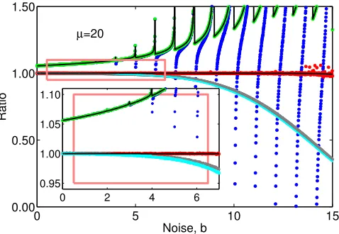
the noise-corrected ratio calculated in four ways: (i) conven-tionally without data rejection (equation 3), (ii) convention-ally with rejection when the denominator is zero or negative (equation 7), (iii) Beale’s estimator, and (iv) quasi-unbiased (equation 15) all with µx0=µy0=b. The mean of 106

ra-tio estimara-tions is plotted for each value of the noise, which is incremented in steps of 0.01. The simulated quasi-unbiased ratios are closer to unity (no bias) than either of the conven-tional ratios or Beale’s estimator over the entire range of b, although significant scatter does occur for large b (see cap-tion). Beale’s estimator (equation 5) on the noise-corrected data requires, for each of the 106_{simulated ratio estimations,}

the variance, covariance and mean intensities to be calculated. We calculate these statistics from a dataset ofnsimulated data pairs,_{xi,yi;i=1. . .n}, and to make the comparison with the

other estimators fair we draw these from a Poisson distribution with mean value 20/n, from which noise ofb/nis subtracted.

0.000 0.002 0.004 0.006 0.008

3.65 3.66 3.67 3.68 3.69

(mean counts of 10B in integration period)−1

11

B/

10

B

(a)

3.658 →

y=3.487 x + 3.658

0.000 0.002 0.004 0.006

0.2730 0.2735 0.2740 0.2745 0.2750

(mean counts of 11B in integration period)−1

10

B/

11

B

(b)

0.2733→

y=0.2493 x + 0.2733

Fig. 1Boron isotope ratios (a)11_B/10_{B and (b)}10_B/11_{B as a} function of the mean number of counts per integration period showing the conventionally computed ratios in blue and the novel

Beale’s estimator is now

r3=n 1_Ân

i=1x0i

n 1_Ân i=1y0i

0

@1+

cov(x_i,y_i)

n 1_Ân

i=1x0iÂni=1y0i 1+ var(yi)

n 1_(Ân i=1y0i)2

1

A, (16)

where

x0

i=xi b/n (17)

and similarly for y0

i. A value ofn=10 is used for the

simu-lation of figure 2. A simplified variation on Beale’s estimator for Poisson data, r0

3, which is independent ofn, may be

ob-tained by substituting n!1, cov(xi,yi)!0, var(yi)!Y,

x0

i!X bandy0i!Y bgiving,

r0

3= _{Y b}X b

+_{Y b}Y

!

. (18)

These substitutions are arrived at by noting that, for in-dependent Poisson distributions, E{cov(X,Y)} = 0 and

E{var(Y)}=E(Y). Simulations of bothr3andr03are included

in figure 2. Note that for zero noise,r0

3=X/(Y+1), i.e.

iden-tical tor0_{(equation 15), and forb>0 the (absolute) bias ofr}0

3

is marginally greater (more negative) than that ofr3.

0 5 10 15

0.00 0.50 1.00 1.50

Noise, b

Ratio

µ=20

0 2 4 6

0.95 1.00 1.05 1.10

Fig. 2Monte-Carlo simulation of(X b)/(Y b)(blue), (X b)/(Z b)(green), Beale’s estimator (grey, see main text), simplified Beale’s estimatorr0

3(cyan, equation 18) and the novel

quasi-unbiased ratio,r0_{(red, equation 15) withµx0=µy0=b,}

whereXandYare independent Poisson variables with means,µx andµy, equal to 20 andZ=Y forY>band rejected otherwise. For each data point the simulation computes the mean over 106_samples. Rare single events whereY is small can significantly shift the mean

r0_{for large values ofbgiving rise to the observed scatter in the red}

[image:5.612.307.546.156.323.2]

data forb&10. Black lines show the theoretical behaviour in the cases of the green and red data. Much of the blue data are obscured behind the green. The noise,b, is incremented in steps of 0.01.

Figure 3 compares the variance ofr0_{(equation 15) with that} of r (equation 7) as a function of mean signal, µx =µy= µ, for three different noise to signal ratios. Over the plot-ted parameter range the variance ofr0 _{is always the smaller} (var(r0_{)/var(r)<1) and, therefore, moreefficientratio} esti-mator.

100 101 102

0.0 0.2 0.4 0.6 0.8 1.0

Noise / Signal

b/µ= 0%,5%and10%

Signal, µ

Var (r’) / Var (r)

Fig. 3Variance ofquasi-unbiased ratio,r0_{(equation 15), divided by}

the variance ofr= (X b)/(Z b)as a function of mean signal, µx=µy=µ, for relative noise,b/µ=0, 5% and 10% showing that the variance inr0_{is always smaller than that of the conventional}

ratio,r, over this range of parameters.

4 Discussion

Quasi-unbiased ratios offer advantages over conventional methods of calculating noise-corrected ratios of ion-counting measurements, namely, (i) an exponentially small statistical bias, (ii) no need to sacrifice within-analysis information by summing counts over entire analysis before taking the ratio, (iii) insensitivity to common-mode changes in signal intensity, (iv) no mathematical singularities, and (v) good stability even with low signal to noise ratios(&2).

Ratio bias has increasing importance in isotope ratio mea-surements since the scientific demands lead researchers to strive for ever higher precisions on small quantities of sample. This is particularly the case in secondary-ion mass spectrom-etry (SIMS) where, because of low blanks, very low count rates are acceptable. In studies on short-lived radionuclides (SLRs) (e.g. see7–10_{) the bias is particularly insidious as it can}

give rise to an apparent linear relationship between measure-ments of the daughter nuclide and a proxy for the parent nu-clide on a so-called ‘isochron’ plot. To illustrate, consider the SLR60_{Fe which decays to}60_{Ni. A suite of measurements are}

[image:5.612.44.283.376.541.2]

plot is made of the daughter,60_{Ni, against the parent element,}

Fe. Both are plotted as ratios using some stable isotope of Ni as the denominator. A straight line with positive slope (the isochron) indicates that60_{Fe was present at the time the Fe and}

Ni were fractionated between the phases. It is sometimes the case that most or all of the variation in Fe/Ni is controlled by the Ni content which, since it appears in the denominator on both axes, will give rise to a linear relationship in the data as a consequence of the bias, adding to the positive slope due to in-growth of60_{Ni. Husset al.}11_{have recently reported this}

prob-lem with some of their own published data on the60_Fe–60_Ni

system concluding that in some, but not all, samples their pub-lished estimates of initial60_{Fe can no longer be distinguished}

from zero. They also discuss the likely size of any corrections to other published work on10_Be, 26_{Al and}53_{Mn concluding}

that any changes to the published conclusions are small ex-cept for one older study on the Mn–Cr system in pallasites.

Note that, where internally-normalised ratios are calculated, i.e. where a third isotope is used to correct for mass-bias, the magnitude of the statistical bias can increase or decrease, de-pending on the relative mass differences, by propagation of the bias of the normalising ratio. For example and assuming a linear mass bias law, in the case of60_Ni/61_{Ni normalised to} 62_Ni/61_{Ni the statistical bias on}60_Ni/61_{Ni increases by a factor}

of two, whereas using62_{Ni as the denominator the statistical}

bias on60_Ni/62_{Ni stays the same magnitude but changes sign}

as it does in the case of26_Mg/24_{Mg normalised to}25_Mg/24_Mg.

For53_Cr/52_{Cr normalised to}50_Cr/52_{Cr the statistical bias}

in-creases by a factor of 1.5.

Studies where mass-bias correction is made by sample– standard bracketing are potentially susceptible to statistical bias in cases where there are differences in analyte concentra-tion (ion count rate) between sample and standard. Standards are usually chosen to have analyte concentrations high enough that good precision can be achieved in a short time under the same analytical conditions employed on the sample. Where ion counts are higher on standards than samples and ratios are calculated conventionally, the statistical bias will result in systematically high ratios reported on samples corrected by sample-standard bracketing. In short, sample-standard brack-eting does not necessarily eliminate the bias.

Husset al.11 _{rightly point out that ratio bias is a problem}

that the community will have to be aware of to avoid this source of systematic error in future work. However, we dis-agree that the best solution is necessarily to sum the counts over the entire analysis before taking the ratio (with or with-out using Beale’s ratio estimator), or to correct for the bias based upon equations 4 or 12, for the reasons (i) – (v) given at the beginning of this discussion, but rather to use equation 15 to compute the ratior0_{at each measurement cycle.}

It may seem laborious to have to evaluate the Kummer con-fluent hypergeometric function for every measurement cycle

but this should not be particularly so if (i) a good library of special functions is available to the software developers or (ii) the signal to noise ratio is sufficiently high to be able to trun-cate the infinite series of equation 14 to yield an approximate value forM(1,Y+2,µ0). The truncation error,en, using an

upper summation limit ofn 1 in equation 14 is given by,

en= •

Â

k=n

µk

0

(Y+2)k. (19)

Leta =µ0/(Y+2)be subject to the constraint 0a <1.

This constraint is not severe: it is sufficient only that the signal is at least as large as the mean noise (and both are positive). Since(Y+2)k (Y+2)kwe may write,

en •

Â

k=n

ak ₍₂₀₎

 a

n

1 a. (21)

Makingnthe subject of the inequality,

n log{en(1 a)}

log(a) . (22)

Therefore, if we wish to calculateM(1,Y+2,µ0)with a

trun-cation error no larger thannwe can use

n=

⇠_log

{n(1 a)_} log(a)

⇡

(23)

and

M(1,Y+2,µ0)⇡

n 1

Â

k=0

µk

0

(Y+2)k. (24)

E.g.n=10 4,Y=10 andµ0=0.5 givesn=3 and truncation

error,en=6⇥10 5_{, smaller thannas required.}

Acknowledgements

The SIMS data in figure 1 were collected at the Edinburgh Ion Microprobe NERC Facility on a sample provided by Dr. Laura Foster of the University of Bristol. Dr. Coath is supported in this work by STFC grant ref. ST/F002734/1.

Appendix

A.1 The expectation value of1/Zl

ForZdistributed as a truncated Poisson distribution (equation 6) we have

E(1/Zl) =N

Â

•

j=l

al(j)P(y0+j+1,µ)

where,

P(a,z) =g(a,z)/(a 1)! a=1,2, . . . is the normalised incomplete gamma function andgis the in-complete gamma function3_{. The coefficientsa}

l(j)are given

byl 1 nested summations

al(j) =j!·(1/j) j 1

Â

j1=l 1

(1/j1)

j1 1

Â

j2=l 2

(1/j2). . .

j_{l 2} 1

Â

j_{l 1}=1

(1/jl 1)

(26) or, alternatively, byal(j) =j!bl(j)and the recursion

bl+1(j) =

(

1/j forl=0;

(1/j)Â_kj₌1_lbl(k) forl 1. (27)

The proof of equation 25 can be subdivided into proofs of

1/Zl ₌

Â

•

j=l

al(j)

(Z+1)j (28)

and E(1/(Z+1)j) = _µN_j·P(y0+j+1,µ) (29)

where we have used Pochhammer’s symbol,(Z+1)j= (Z+

1)(Z+2). . .(Z+j). The proof of equation 29 yields easily as follows. From the probability distribution function defined in equation 6 it follows that

E(1/(Z+1)j) =Ne µ

•

Â

z=y0+1

µz

(z+1)jz!

=Ne µ µj

•

Â

z=y0+1

µz+j

(z+j)!

= N

µj 1 e µ y0+j

Â

z=0

µz

z!

!

=_µN_j·P(y0+j+1,µ)

where we have used Arfken12_{equation 10.70 in the final step}

completing the proof.

Equation 28 yields as follows. Denote

{p}j=1/(p)j.

Given integerss 0 andt swe have

Â

sz<t{

z+1}j= ({s+1}j 1 {t+1}j 1)/(j 1) (30)

Proof: fors=t, obviously RHS = LHS = 0. Fort>s, by induction ont susing

RHS(s,t) RHS(s,t 1) = ({t}j 1 {t+1}j 1)/(j 1)

= ((t+j 1){t}j t{t}j)/(j 1)

=_{t_}j

=LHS(s,t) LHS(s,t 1) ⇤

Define

hl(j) =

•

Â

jl 1=j+1

(1/jl 1)

•

Â

jl 2=jl 1+1

(1/jl 2). . .

•

Â

j0=j1+1

(1/j0){j0+1}n, (31)

that is,lnested summations where each lower limit is the next outer summation variable. We have explicitly

hl(j) =1/nl· {j+1}n. (32)

Proof: by induction on l. From the definition (equation 31) follows the recursion

hl(j) = (

{j+1}n forl=0;

•k=j+1hl 1(k)/k forl 1. (33)

The result is trivial forl=0; forl>0, substituting the RHS value for hl 1(k) (equation 32) into the recursion (equation

33),

hl(j) =

•

Â

k=j+1

1/nl 1· {k+1}n/k

= 1/nl 1_· •

Â

k=j+1{

k_}n+1

= 1/nl· {j+1}n

using equation 30 witht!•,s!j, and j!n+1. ⇤ Changing the order of summation and combining equations 31 and 32 gives

{j+1}n/nl=

•

Â

j0=j+l

(1/j0){j0+1}n j0 1

Â

j1=j+l 1

(1/j1)

j1 1

Â

j2=j+l 2

(1/j2). . .

jl 2 1

Â

jl 1=j+1

(1/jl 1).

With j_!0 and substituting using the identityn!_{j0+1}n⌘

j0!/(n+1)j0,

1/nl= •

Â

j0=l

j0!(1/j0)/(n+1)j0

j₀ 1

Â

j1=l 1

(1/j1)

j1 1

Â

j2=l 2

(1/j2). . .

jl 2 1

Â

jl 1=1

(1/jl 1).

References

1 K. Coakley, D. Simons and A. Leifer,International Journal of Mass Spec-trometry, 2005,240, 107–120.

2 R. C. Ogliore, G. R. Huss and K. Nagashima,Nuclear Inst. and Methods in Physics Research, B, 2011,269, 1910–1918.

3 Digital Library of Mathematical Functions, National Institute of Stan-dards and Technology, 2010, ch. 8.

4 Digital Library of Mathematical Functions, National Institute of Stan-dards and Technology, 2010, ch. 13.

5 A. Prudnikov, Y. Brychkov and O. Marichev, inMore Special Functions, Gordon and Breach, 1986, vol. 3, p. 409.

6 I. Gradshteyn and I. Ryzhik, inTables of Integrals, Series and Products, Academic Press, 7th edn., 2007, p. 1023.

7 K. McKeegan, M. Chaussidon and F. Robert,Science, 2000,289, 1334– 1337.

8 E. Kurahashi, N. T. Kita, H. Nagahara and Y. Morishita,Geochimica et Cosmochimica Acta, 2008,72, 3865–3882.

9 P. Hoppe, D. Macdougall and G. W. Lugmair,Meteorit Planet Sci, 2007,

42, 1309–1320.

10 S. Tachibana and G. Huss,Astrophys J, 2003,588, L41–L44.

11 G. Huss, R. Ogliore, K. Nagashima, M. Telus and C. Jilly, 42nd Lunar and Planetary Science Conference, #2608, 2011.