A self consistent phase space distribution function for the anisotropic dark matter halo of the Milky Way

arXiv:1311.5477v1 [astro-ph.CO] 21 Nov 2013

Milky Way

Mattia Fornasa and Anne M. Green

School of Physics and Astronomy, University of Nottingham, University Park, Nottingham, NG7 2RD, United Kingdom

Dark Matter (DM) direct detection experiments usually assume the simplest possible ‘Standard Halo Model’ for the Milky Way (MW) halo in which the velocity distribution is Maxwellian. This model assumes that the MW halo is an isotropic, isothermal sphere, hypotheses that are unlikely to be valid in reality. An alternative approach is to derive a self-consistent solution for a particular mass model of the MW (i.e. obtained from its gravitational potential) using the Eddington formalism, which assumes isotropy. In this paper we extend this approach to incorporate an anisotropic phase-space distribution function. We perform Bayesian scans over the parameters defining the mass model of the MW and parameterising the phase-space density, implementing constraints from a wide range of astronomical observations. The scans allow us to estimate the precision reached in the reconstruction of the velocity distribution (for different DM halo profiles). As expected, allowing for an anisotropic velocity tensor increases the uncertainty in the reconstruction of f (v), but the distribution can still be determined with a precision of a factor of 4-5. The mean velocity distribution resembles the isotropic case, however the amplitude of the high-velocity tail is up to a factor of 2 larger. Our results agree with the phenomenological parametrization proposed in Mao et al. (2013) as a good fit to N-body simulations (with or without baryons), since their velocity distribution is contained in our 68% credible interval.

I. INTRODUCTION

The goal of Milky Way (MW) mass modelling is to build a model of our Galaxy in terms of the density distributions of its components [1–6]. Mass models are the first step towards more complete dynamical descriptions of the MW in which the phase-space distribution F(x,v) [7], consistent with the

potential, is determined. The topic has recently received re-newed interest (see, e.g., Refs. [8–20]). This is in part due to the importance of accurate determinations of the local Dark Matter (DM) density,ρ0, and circular velocity,Θ0, for Weakly Interacting Massive Particle (WIMP) direct detection experi-ments, which aim to detect the recoil energy deposited in a detector when WIMPs scatter offnuclei (see Refs. [21–23] for recent reviews).

The direct detection energy spectrum and its annual mod-ulation, due to the Earth’s orbit [24], depend on the local velocity distribution f (v) = F(x_⊙,v)/ρ(x_⊙), where x_⊙ de-notes the position of the Sun andρ(x) is the DM density (see Refs. [25–30], among others). Direct detection experimen-tal data are usually analysed assuming the so-called Standard Halo Model (SHM), which describes the MW as an isotropic isothermal sphere with local densityρ0=0.3 GeV cm−3and a Maxwellian-Boltzmann velocity distribution

f (v)= 1

(2π)3/2_σ3exp −

v2

2σ2

!

, (1)

with velocity dispersionσ = Θ0/

√

2 and Θ0 = 220 km s−1. This model is unlikely to be a good approximation to the real MW DM halo. N-body simulations produce halos with velocity distributions which deviate systematically from a Maxwellian [26, 31].

Finding an appropriate phase-space distribution for the DM halo of the MW when you know its gravitational potential (i.e. obtaining a complete dynamical model for the Galaxy from its mass model) can be done under certain simplifying

assump-tions. For instance the phase-space distribution of a spheri-cally symmetric system, with an isotropic velocity tensor, can be written as function of the energy E alone [7]. In this case one can solve for F(E), using the Eddington equation [32]. The solution will be self-consistent, in that F(E) and the grav-itational potential of the system,Φ(x), satisfies Boltzmann’s equation (e.g. Refs. [13, 33, 34]).

For the more general case of a spherical system with an anisotropic velocity tensor, the phase-space distribution func-tion also depends on the modulus of the angular momen-tum, L. Often a parametric form is considered for F(E,L)

and one can still find the set of parameters that corresponds to a self-consistent solution. Ref. [35] assumed that the phase-space distribution is separable in the two variables (i.e.

F(E,L) = FE(E)FL(L)) and proposed a particularly

conve-nient expression for FL(L) that depends on three parameters

and can fit the radial dependence of the velocity anisotropy parameterβ(r)

β(r)=1₋ σ 2 t 2σ2

r

, (2)

in the case of halos formed in N-body simulations, whereσt andσr are the tangential and radial velocity dispersions. In this paper, we apply the formalism developed in Ref. [35] in the context of the DM halos of galaxy clusters to the MW DM halo (see also recent work in Ref. [20] for an alternative ap-proach to anisotropy). The first step is to build a mass model of the MW, c.f., e.g., Refs. [11, 13, 15, 18], using a wide range of astronomical observations to constrain the gravita-tional potential of the MW and, therefore, the DM density profile. Our inferred knowledge ofΦ(x) will then be used to derive self-consistent solutions for F(E,L), using the

three-parameter form of FL(L) introduced in Ref. [35].

constructing a mass model of the MW, where the density profiles of the different components of the MW are written as functions of a number of free parameters which are con-strained using astronomical observations. In this case, we also parametrize FL(L) and use our knowledge of the gravitational

potential to derive self-consistent solutions for F(E,L), and

therefore f (v).

This is a different approach to that which has previously been used for anisotropic halos (e.g. Refs. [25, 30, 36]) where the components of the DM velocity dispersion tensor have been found by solving the Jeans equation [7]. The velocity distribution is reconstructed with a remarkable precision, but the resulting solutions are not necessary self-consistent. In our approach, the Jeans equation is automatically satisfied (thanks to the Jeans theorem) without having to impose it explicitly.

The paper is structured as follows. In Sec. II we introduce our mass model for the MW, listing the free parameters of the model in Sec. II A and the observations we use to constrain the parameters in Sec. II B, while Sec. II C describes the statisti-cal techniques employed in the scans. Sec. III is devoted to the discussion of the resulting constraints on the mass model parameters. In Sec. IV we present our technique for obtaining self-consistent anisotropic phase-space distributions, F(E,L),

and we apply it to the MW model found in the previous sec-tions. In Sec. V we discuss our results and in Sec. VI we summarize our conclusions.

II. MASS MODELS OF THE MILKY WAY

In this section we discuss how we obtain a viable mass model for the MW. Our general approach follows previous work e.g., Refs. [11, 13, 15, 18], with some differences in the details of how observations are implemented and in the modelling of the mass components.

The basic idea is to model the dynamically important com-ponents of the MW with physically motivated parametrisa-tions, and then constrain the free parameters using a range of observations. We use a nested sampling algorithm to search the parameter space, and find the Bayesian probability distri-bution functions for the free parameters. If the observational data used are informative enough, the final results will be a precise MW model in agreement with observations, as well as estimates of the residual uncertainties in the model parame-ters.

In the follow subsection (Sec. II A) we describe the compo-nents of our MW mass model, including the free parameters. In Sec. II B we list and discuss the different observations and their implementation. Finally in Sec. II C we give some de-tails about the sampling technique.

A. Milky-Way mass contributors

Our mass model of the MW follows closely that proposed in Ref. [11], and has four components:

• stellar disk: Following Ref. [11], we model the

stel-lar disk with a single component thin disc with density

profile (in cylindrical coordinates):

ρd(R,z)= Σd 2zd

exp(₋R/Rd) sech2

z zd

!

, (3)

which is in agreement with the fit to the COBE Dif-fuse Infrared Background Experiment data discussed in Ref. [37]. The scale length in the z-direction is fixed at

zd = 0.34 kpc, since the dynamical constraints consid-ered here are insensitive to small variations in its value, while the normalization,Σd, and the radial scale length,

Rd, are left as free parameters.

Ref. [15] considered a mass model with two disks, a thin and a thick one. Since the stellar components are not the focus of our investigation, we consider a model with a single disk which has fewer free parameters (see also Sec. II B 2).

The gravitational potential produced by Eq. (3) is ax-isymmetric (see, e.g. Ref. [19]), however, for simplic-ity, we work under the assumption of spherical symme-try, leaving the investigation of non-spherical Galactic models to future work. Thus, the disk gravitational po-tential at a certain distance r from the center of the MW can be well approximated by GR∞

r dr Md(<r)/r, where Md(<r) is the disk mass enclosed in a sphere of radius

r. The deviation of the spherical gravitational potential

from the true axisymmetric one (for the best-fit point for a Navarro-Frenk-White DM halo, see later) is max-imal near the Galactic Center and is less than 10% for distances larger than 2.2 kpc1.

• bulge/bar: As in Ref. [11], we consider an

axisymmet-ric version of the model proposed in Ref. [38]:

ρbb(x,y,z)=ρbb(0)

h

s−_a1,85exp(₋sa)

+exp(₋0.5s2_b)i, (4)

with

s2a=

q2_b(x2+y2)+z2

z2 b

, (5)

and

s4_b=

     

x2+y2 x2

b

     

2

+ z

zb

!4

. (6)

The two terms represent the bar and the bulge, respec-tively. Their parameters are set to qb = 0.6, zb = 0.4 kpc (8 kpc/R0) and xb =0.9 kpc (8 kpc/R0), rescal-ing to arbitrary R0, the distance of the Sun from the

1_{This is the deviation with respect to the average of the axisymmetric}

Galactic Center, as suggested by Ref. [38]. The normal-izationρbb(0) is left free. Another viable model for the bulge/bar system can be found in Ref. [39]. This com-ponent is always subdominant in our results and there-fore we do not expect our results for the local DM distri-bution to be sensitive to the details of the bulge/bar den-sity parametrization. As for the disk, the gravitational potential of the bulge/bar is assumed to be spherical and is obtained by computing the enclosed mass.

• interstellar medium: The model for the interstellar

medium is kept fixed, without any free parameters. The mass density of molecular hydrogen H2, as well as the HI and HII components, is modelled as in Ref. [40], based on the observations presented in Ref. [41].

• DM halo: Insight into the density profile of the DM

halo comes mainly from the study of synthetic halos formed in N-body simulations [42–45]. We consider three different spherically symmetric parametrizations for the DM density profile: a Navarro-Frenk-White (NFW) profile [46]

ρχ(r)=ρs

r rs

!−1

1+ r

rs

!−2

, (7)

an Einasto profile [47]

ρχ(r)=ρsexp − 2 α

" r rs

!α

−1

#!

, (8)

and a Burkert profile [48]

ρχ(r)=ρs 1+

r rs

!−1

1+r 2

r2 s

!−1

. (9)

The scale radius, rs, is related to the radius at which the logarithmic derivative of the density profile is equal to₋2, whileρsfixes the normalization. The NFW and Burkert profiles only have two free parameters (rsand

ρs) while the Einasto profile has an additional parame-ter,α, which controls the curvature of the profile. The NFW and Einasto profiles have inner cusps and pro-vide good fits to the density profiles of halos formed in DM-only N-body simulations. Baryons are likely to play an important role in determining the DM distri-bution in the inner regions. However, simulating bary-onic physics, and forming realistic galaxies, is a difficult problem (see, e.g., Refs. [49, 50] for recent progress) and it is not yet clear how baryonic physics will af-fect the DM density profile. The Burkert profile has a central core, a possibility that seems to be preferred by observations of dwarf Spheroidal [51] or Low-Surface Brightness galaxies [52].

To compare with other mass models and other DM halo constraints present in the literature, we will also calcu-late the concentration parameter c =rvir/rs, where rvir is the virial radius, i.e. the radius within which the aver-age density of the halo is∆, the virial overdensity, times

the critical density of the Universe. In a flatΛCold DM Universe with matter density parameter Ωm = 0.227 [53] at z=0,∆ =94 [54]2_.

Unlike Ref. [13] we do not include uncollapsed baryons in our MW model, as their distribution is highly uncertain and the majority are thought to be in the warm-hot intergalactic medium (see e.g. Ref. [55]). See Sec. III for further discus-sion.

There are five additional quantities that will be needed when implementing the observational constraints (see Sec. II B). These are R0,β∗(the velocity anisotropy of stellar halo

tracers, see Sec. II B 6) and the three components of the ve-locity of the Sun with respect to the Rotation Standard of Rest (see Sec. II B 1), VRSR

⊙ = (U

RSR

⊙ ,V

RSR

⊙ ,W

RSR

⊙ ), in a system of

coordinates where the first axis points towards the Galactic Center, the second along the direction of Galactic rotation and the third is perpedicular to the Galactic plane.

B. Experimental constraints

As emphasised by Ref. [15] the fact that different experi-mental constraints use different underlying assumptions is an issue when constructing a MW mass model. In principle the best approach would be to use the raw data, rather than values of derived quantities, however in practice this is not possible. Still, where possible, we avoid using constraints which make specific assumptions, e.g. a fixed value of the solar radius, R0.

1. Local circular velocity

Measurements of the local circular velocity,Θ0, can be di-vided into two categories: those that measure the rotation ve-locity of the Sun, Vφ,⊙, by observing the proper motion of

an object (or a population of objects) at rest at the Galactic Center, and those that measure the difference between the two Oort constant, A₋B = Θ0/R0, from the proper motions of tracers.

Ref. [56] measured the proper motion of Sgr A⋆ with an extremely good accuracy of approximately 0.4%: µl =

(₋6.379_±0.026) mas yr−1_{. The local circular velocity can then} be calculated using R0, and the velocity of the Sun with re-spect to the so-called Rotation Standard of Rest (RSR), VRSR

⊙ ,

i.e. the rotation velocity of a circular orbit in the axisymmet-ric approximation of the gravitation potential [57, 58]. On the other hand, Ref. [59] measured A₋B with 3% accuracy using

the motion of 220 Cepheids detected by the Hipparcos satel-lite: A−B=(27.2±0.9) km s−1kpc−1.

The two techniques appear to lead to inconsistent values of

Θ0, depending on the value of V_⊙RSR assumed. Traditionally it has been assumed that the Local Standard of Rest (LSR,

2_{Using the more recent value ofΩ}

i.e. the orbit of local stars with “zero velocity dispersion”, obtained by extrapolating to σR = 0 the definition of the asymmetric drift, [58, 60]) moves on a circular orbit. If this is true then the rotational component of the Sun’s velocity with respect to the LSR, VLSR

⊙ , coincides with V⊙RSR, and can

be used to estimate Θ0 from the measurement of Vφ,⊙.

Us-ing VLSR

⊙ =5 km s−

1_{, from the analysis in Ref. [5] of}

Hippar-cos data and R0 = 8.0 kpc from Ref. [61], Ref. [56] find Θ0/R0 = (29.4±0.2) km s−1kpc−1, significantly larger than the value quoted in Ref. [59] of (27.2_±0.9) km s−1kpc−1. However, using line-of-sight velocities of more than 3000 stars observed by the APOGEE survey, Ref. [58] found

VRSR

⊙ =Vφ,⊙−Θ0 =23.9₋+5₀._.1₅km s−1(assuming a flat rotation curve). This is significantly larger than even the revised value of VLSR

⊙ of 13 km s−

1 _{[62], found taking into account the}

ra-dial metallicity gradient. Ref. [58] discussed two possible reasons for this discrepancy. For instance, the LSR would dif-fer from the RSR if the orbit of the LSR is not circular (due, for instance, to large-scale non-axisymmetric streaming mo-tions). Alternatively, VLSR

⊙ could be significantly larger than

previously thought. Using the value of VRSR

⊙ =23.9 km s− 1

quoted in Ref. [58], the value ofΘ0/R0found from the measurement of the proper motion of Sgr A⋆in Ref. [56] drops to 27.1 km s−1kpc−1, con-sistent with both the value in Ref. [59] value and the measure-ment ofΘ0from Ref. [58].

In light of this, we constrain the circular velocity by im-posing the measurement of the proper motion of Sgr A⋆ by Ref. [56], assuming the value of VRSR

⊙ quoted before from Ref.

[58] (see also Sec. II B 7). We also follow Ref. [11] by using

A+B=∂Θ(r)/∂r_|r=R0=(0.18±0.47) km s

−1_kpc−1_.

2. Local surface density

The total integrated local surface density, within a vertical distance z of the Galactic plane, is defined as

Σ(R0,z)=

Z z

−z

ρtot(R0,z) dz, (10)

whereρtot is the total mass density of the MW. A demonstra-tion that this quantity continues increasing for z larger than a few times the disk scale length, zd, would be very strong evidence for the presence of DM at the Solar radius. The lo-cal surface density can be estimated by means of the Poisson equation, once the vertical force, Kz, is determined. We use

the values, derived from the kinematics of stellar tracers, from Ref. [63] and Ref. [64] ofΣ_∗(R0) = (48±8)M⊙pc−2 and Σ(R0,1.1 kpc) = (71±6)M⊙pc−2 for the visible component

and the total mass within 1.1 kpc, respectively. These values are consistent with more recent analyses, e.g. Refs. [65–69].

Ref. [70] used the data from Refs. [71–73] to derive lower limits on the local surface density up to 4 kpc. We do not use these results since they are, strictly speaking, only lower limits and also because of the large residuals in the fit to UW (see Fig. 2 of Ref. [71]).

3. Terminal velocities

The inner rotation curve of the MW, i.e. inside the Solar radius, can be constrained by measurements of the so-called terminal velocities: along each line-of-sight towards Galac-tic longitude l there is a point at which the distance from the Galactic Centre is smallest. Under the assumption of circular motion, the modulus of the line-of-sight velocity is largest for objects at this minimum distance that are moving on an orbit that is tangential to the line-of-sight. This maximal velocity is normally referred to as the terminal velocity and can be used to directly constrain the rotation curve of the MW, at that spe-cific minimal distance.

Measurements of terminal velocities are obtained from the observation of the spectral line of atomic hydrogen HI (see, e.g. Ref. [74]) or of CO [75]. We consider the data set in Ref. [74], excluding all the points with_|sin l_| < 0.35◦_{, where the}

assumption of circular motion is not valid due to the presence of the Galactic bar. A constant experimental error of 7 km s−1 is assumed for each of the remaining data points (following Ref. [11]).

4. Microlensing

Microlensing observations constrain the gravitational po-tential of the MW since they provide us with a probe of the mass density in compact objects in the direction(s) of observa-tion. The impact of microlensing data on the reconstruction of the MW potential has been studied in Ref. [14]. We consider the same 10 measurements of the optical depth_hτ_idiscussed in that paper, coming from the MACHO [76], OGLE-II [77] and EROS [78] collaborations. The distribution of the gravi-tational lenses is assumed to follow the matter density of the disk and the bulge/bar, while the distribution of sources de-pends on the particular microlensing events (see Ref. [14] for more details).

5. Proper motion of masers in high-mass star-forming regions

Ref. [79] found that the 18 masers they analyzed were orbiting around the Galactic Center with (on average) Vs ∼

−15 km s−1. However Ref. [80] argue that it is more likely that VLSR

⊙ ≈11 km s−

1_{, as advocated by Ref. [62], rather than}

the value of VLSR

⊙ ≈5 km s−

1 _{[5] used by Ref. [79]. Note that}

the value of VLSR

⊙ proposed in Ref. [62] is still smaller than the

value in Ref. [58] of VRSR

⊙ =23.9 km s− 1

which we adopt, see Sec. II B 1.

We implement the information from the motions of masers, following Ref. [80], by marginalizing over the peculiar veloc-ities and parallaxes of the masers. We assume that the com-ponents of the peculiar velocities have a Gaussian probability distribution with zero mean and∆v=10 km s−1. A Gaussian distribution is also assumed for the parallax, with the mean and dispersion coinciding with the measured value ofπand the experimental error, respectively, for each maser.

We consider a total of 33 masers from Refs. [79, 81–90].

6. Velocity dispersion of halo stars

Ref. [91] selected a sample of more than 2000 Blue Horizontal-Branch stars observed by the Sloan Digital Sky Survey and computed the dispersion of the line-of-sight ve-locity in 10 bins in distance from the Galactic Center, from 5.0 to 60.0 kpc. They compare these measurements with the results of two cosmological galaxy formation simulations of MW-like galaxies to infer the rotation curve of the MW up to 60.0 kpc.

We follow Ref. [11] and directly use the binned line-of-sight velocity dispersion data. We do not use the results of the simulations, however our analysis is based on the follow-ing three assumptions, that receive validation from the sim-ulations used in Ref. [91]: i) the dispersion of the line-of-sight velocity can be used as an estimate of the radial velocity dispersion, ii) the stellar densityρ_∗ is well fitted by a r−3.5 power law and iii) the stellar velocity anisotropy parameter β_∗is constant over the range of distances considered. Under these assumptions, one can solve the Jeans equations for the Blue Horizontal-Branch stars analyzed by Ref. [91] to obtain an expression for the radial velocity diversion of the stars [11]:

σ2r,∗(r)=

1

r2β∗_ρ∗(r)

Z ∞

r

ds s2β∗−1_ρ

∗(s)Θ2(s). (11)

The 10 velocity dispersion data points in Ref. [91] can thus be used to constrain the circular velocity at large radii. Note that the constant velocity anisotropy parameter of the stars,β_∗, is a free parameter in our scans.

7. Nuisance parameters

The Sun’s distance from the Galactic Center, R0, as well as the three components of the velocity of the Sun with respect to the RSR are included in the scan as nuisance parameters. We assume the U and W components of the Sun’s velocity with respect to the RSR and LSR are identical (see Sec. II B 1).

We also assume a Gaussian probability distribution for each nuisance parameter, with a mean value and dispersion corsponding to the measured value and experimental error, re-spectively:

• R0=(8.33±0.35) kpc, inferred from the observation of stellar orbits around the Galactic Center [92].

• URSR

⊙ =(11.1±1.0) km s− 1_[62].

• VRSR

⊙ =(23.9±5.1) km s− 1

[58], see Sec. II B 1.

• WRSR

⊙ =(7.25±0.50) km s− 1_[62].

8. Other observations

Refs. [93, 94] estimated the total mass of the MW from the kinematics of satellite galaxies, globular clusters and (in the case of Ref. [94]) individual stars, considered as tracers of the underlying gravitational potential. Their results have an accu-racy of approximately a factor of 2, pointing towards a total DM halo mass of around_∼1012_M

⊙. However these estimates

are obtained using assumptions which we do not make in our analysis (e.g. a fixed value of R0 and of the Solar RSR ve-locity). Moreover, the results in Ref. [93] become very prior dependent as soon as the value ofΘ0is left free, as it is in our scans since it depends on the mass model. Thus, we decide not to consider such results.

Ref. [95] found, using high velocity stars from the RAVE survey, that the local escape velocity lies between 492 and 587 km s−1 (at 90% confidence). No constraint on the es-cape velocity is included in our scan since Ref. [15] argued that assuming that these stars are in a steady state (as done in Ref. [95]) is probably unrealistic. Moreover, the range quoted could be even larger depending on the parameterisation of the high speed tail of the stellar velocity distribution.

Finally, the mass model in Ref. [15] used two additional constraints from simulations. Namely the concentration of MW-like halos from Ref. [96] and the following relation for the ratio of stellar mass, M⋆, to DM mass, Mχ,:

M⋆

Mχ

=0.129

      

Mχ

1011.4

!−0.926

+ Mχ

1011.4

!0.129      

−2.44

, (12)

found by Ref. [97] to be a good fit to the Millennium-II sim-ulation. We prefer to include only observational data and thus we do not consider the information coming from N-body sim-ulations. However, in Sec. III we will show the predictions of our mass models for the observables discussed here (i.e. total mass of the MW within 50 kpc and within the virial radius, the escape velocity, the concentration of the MW DM halo and the DM/stellar mass ratio) but not included as data.

C. Sampling technique

intro-Name Range Probability distribution ρs[M⊙pc−3] 10−5, 1.0 log

rs[kpc] 0.0, 100.0 log

Rd[kpc] 1.2, 4.0 log

Σd[M⊙pc−2] 102, 104 log

ρbb(0) [M_⊙pc−3_{] 10}−4_{, 10}2 _log

α 0.1, 0.4 flat

β_∗ -1.0, 0.7 flat

R0[kpc] 6.5, 9.0 Gaussian

URSR

⊙ [km s−

1_{] 1.1, 21.1 Gaussian}

VRSR

⊙ [km s− 1

] -7.76, 32.24 Gaussian

WRSR

⊙ [km s−

1_{] 2.25, 12.25 Gaussian}

β0 -0.5, - flat

β_∞ -0.5, 1.0 flat

kL₀ 10−3_{, 10}3 _log

TABLE I. Parameters defining the multidimensional space over which our scan is performed. The first column is the name of the parameter, the second the range of values considered in the scan and the third indicates the form of the prior probability distribution func-tion. The first section of the table contains the parameters of the MW mass model introduced in Sec. II:ρs fixes the normalization of the DM halo and rs is its scale radius. Rdis the radial scale density of the disc, Σd andρbb(0) determine the normalization of the density profiles of the disk and bulge/bar respectively. Finally,αappears in the Einasto DM halo profile. The second section contains param-eters which are needed to implement the astronomical constraints (see Sec. II B):β_∗is the velocity anisotropy parameter for the Blue Horizontal-Branch stars considered in Ref. [91] (see Sec. II B 6), R0 is the distance of the Sun from the Galactic Center and (URSR

⊙ , V⊙RSR,

WRSR

⊙ ) are the components of the velocity of the Sun with respect to the RSR. The final section contains the parameters which appear in the part of the phase-space distribution function which depends on the angular momentum:β0andβ∞are the velocity anisotropy of the DM halo at r=0 and r=_∞respectively and kL0is a proportionality constant between the parameter L0(entering in the definition of the phase-space density) and rsΘ(rs)

√

ln 2−1/2 (see Sec. IV). We do not indicate here the upper limit forβ0since it depends on the form of the density profile (see Sec. IV).

duced in Sec. II A (note that the quantityαis only applica-ble in the case of the Einasto profile). The distance of the Sun from the Galactic centre, R0, and the components of the Sun’s motion with respect to the RSR, URSR

⊙ , V⊙RSRand W⊙RSR, are

considered as nuisance parameters (see Sec. II B 7). The last three parameters,β0,β∞and kL0, parameterise the part of the phase-space distribution function which depends on the angu-lar momentum and will be introduced in detail in Sec. IV.β0 andβ_∞are the velocity anisotropy parameters at the center of the MW and at infinity, respectively. The third parameter en-tering in the L-dependent part of the phase-space density is a characteristic scale L0. The parameter considered in the scan, however, is the ratio between L0and “scale angular momen-tum” Ls=rsVs=rsΘ(rs)(ln 2−1/2)−1/2.

The second column indicates the range of values considered for each of the parameters and the third column indicates the shape of the prior probability distribution.

The scan is performed using the public code MultiNest

[98], which uses a nested sampling algorithm to determine the Bayesian posterior probability distributions for the param-eters in the scan and functions of these paramparam-eters. The core principle is Bayes’ theorem:

Pr(Θ_|D,H)=Pr(D|Θ,H) Pr(Θ|H)

Pr(D_|H) , (13)

which shows how the so-called prior probability Pr(Θ_|H) of

the parametersΘ(describing our knowledge of the quanti-ties in the context of model H before the implementation of the experimental data D) is updated once we consider the observational information encoded in the likelihood_L(Θ) =

Pr(D_|Θ,H). The result is the posterior probability

distribu-tion funcdistribu-tion (pdf) Pr(Θ_|D,H), which also depends on the

so-called evidence Pr(D_|H). We do not need to include the

ev-idence as it only depends on the data and therefore acts as a normalization constant.

Different choices of prior distributions can affect the fi-nal posterior pdf if the data considered are not constraining enough to overcome the shape of the prior. The third column in Tab. I indicates for each parameter whether we assumed a Gaussian prior distribution (denoted by Gaussian) or a uni-form distribution on a linear scale (flat) or logarithmic scale (log). In the case of the NFW DM halo for some parameters we used both flat and log priors, in order to check that the posterior pdfs do not depend significantly on the choice of the prior. When not explicitly mentioned, all the results presented in the following sections refer to the choice of priors indicated in Tab. I.

We are interested in the probability distributions of particu-lar subsets (normally 1- or 2-dimensional) of the parameters in Tab. I. Two different statistics can be considered to measure such distributions. The so-called posterior pdf of parameter

Θiis found by marginalizing over all the other parameters:

pdf(Θi)= Z

dΘ0dΘ1· · ·dΘi−1dΘi+1· · ·dΘN−1dΘN

×Pr(Θ_|D,H), (14)

where N is the total number of parameters in the scan. On the other hand, the profile likelihood (PL) of parameterΘiis

found by maximizing over the other parameters3_:

PL(Θi)= max

Θ0,Θ1,···,Θi−1,Θi+1,···,ΘN−1,ΘN

L(Θ). (15)

The PL is very sensitive to fine-tuned regions in the param-eter space with a very large likelihood, while the pdf takes into account volume effects where large regions with a mod-erate likelihood are integrated over. It is normally useful to consider both quantities when studying the characteristics of a parameter space [99, 100].

For each parameter we will compute the so-called x%

cred-ible interval, defined so that the each of the two tails outside

3_{One can write similar expressions for the pdf and PL of more than one}

the interval has a probability 0.5x%. We also determine the

x% confidence levels as the region with a likelihood at most

∆χ2_{(x) lower than the likelihood of the best-fit point, where} ∆χ2_{(x) is determined by solving}

x=

Z ∆χ2

0

dyχ2n(y), (16)

whereχ2

n(y) is theχ2 distribution with n degrees of freedom.

We used the SuperBayes package4 _{[101, 102] to compute} the credible intervals and confidence regions and produce the plots presented in the following sections.

We performed our scans using 2000 live-points and a tol-erance of 10−4_{. Ref. [99] showed that such a set-up allows a} good reconstruction of the PL in the context of SuperSymmet-ric models of Particle Physics. The pdf and PL distributions for our scans do not differ much from each other, which con-firms that we have achieved a reliable evaluation of the PL.

III. PARAMETER ESTIMATION FOR THE MILKY WAY MASS MODELS

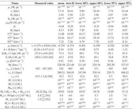
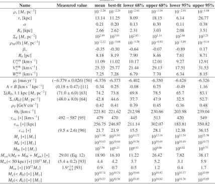
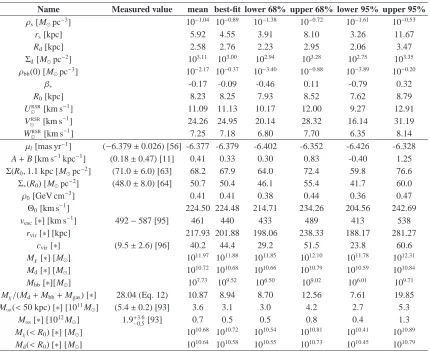
In this section we present the results of our scans, determin-ing the parameters of our MW mass model. Tabs. II, III and IV summarize the results, including mean and best-fit values and 68% and 95% credible intervals, for the NFW, Einasto and Burkert DM halo profiles, respectively. Note that in order to facilitate comparisons with other studies we include derived values of quantities (marked with_∗) that are not considered as experimental data in our scans.

The three mass models associated with the different DM ha-los share the following properties: in the (ρs,rs) plane, lines of

constant Mχ(<R0), the DM mass within the solar radius, are approximately parallel to lines with constantΣχ(R0,1.1 kpc), as well as lines with constant ρ0. Thus, imposing the con-straints on Σ(R0,1.1 kpc) and Σ∗(R0) (fixing, indirectly, the local DM surface density), will select one of those lines (de-termining one degenerate direction in the plane (ρs,rs)) and

will translate into a determination of Mχ(<R0) andρ0. The degeneracy is broken when we include the information on the velocity dispersion, which fixes the DM mass inside larger radii. On the other hand, in the (Σd,Rd) plane, the lines of

constantΣd(R0,1.1 kpc) are not parallel to those with constant

Md(<R0), so that the information onΣ∗(R0) and onΘ0 (con-straining the total amount of matter within R0) act in a com-plementary way. The allowed region in the (Σd,Rd) plane gets

slightly larger when the terminal velocity data are included, since they prefer a less dense disk and a balance has to be made between the constraints onΣ_∗(R0) andΘ0.

Microlensing and the proper motions of masers do not introduce significant addition information to the determina-tion of the mass model. In the case of the microlensing data the baryonic component is already well determined by

4_{http://www.ft.uam.es/personal/rruiz/superbayes/}

the information on the local surface density and the rotation curve. While, for the masers, since we are marginalizing over the velocity of the peculiar motion of each maser, the scan practically has the effect of determining which values of (Us,Vs,Ws) (for each object) provide a good fit to the data,

given a rotation velocity fixed by the constraints on the local surface density and the rotation curve. This result was already discussed by Ref. [103].

The gravitational potential is dominated by the disk for

R <R0, while the DM halo only becomes important around the Sun’s radius. The bulge/bar is always subdominant: the probability distribution for ρbb(0) is almost flat for values smaller than approximately 1 M_⊙pc−3 _{and then goes rapidly} to zero. This means that one should regard the upper end of the 68% and 95% credible contours forρbb as upper limits, while the lower end is practically determined by the range of values scanned.

Fig. 1 shows the posterior pdf for the rotation curveΘ(r). The dark and light blue band indicate the 68% and 95% cred-ible regions, respectively. The solid black line corresponds to the best-fit point and the fact that it falls within the 68% credible interval reflects the similar shape of the pdf and PL contours. The dashed (dotted) line shows the contribution of the DM halo (disk) to the MW rotation curve.

No tension is present between the results of the scans and the experimental data considered. At the best-fit point (inde-pendently of which profile is used for the DM halo) theχ2_is dominated by the proper motion of masers, which is responsi-ble for approximately half of the value ofχ2_.

The results of Tab. II for the case of a NFW DM halo are quite similar to the case of an Einasto halo, since the two parametrizations differ mainly in the inner region, where DM does not dominate the gravitational potential. On the other hand, a larger concentration and a smaller virial mass for the DM halo are obtained for the case of a Burkert profile. This is a consequence of the presence of the core: fixing the local DM density to a common value for the three halo models (as a result of the measurement of the local circular velocity and of the local surface density) implies a lower concentration for the Burkert DM halo. We stress that the goal of this paper is to infer local quantities (specifically the velocity distribution

f (v)), not to determine whether a cuspy or cored profile

pro-vides a better fit to the data. Thus we leave a comparison of the goodness of fit of the different models for future work.

Our results are similar to those of Ref. [11]. The main dif-ference is our value for the local circular velocity, which is_∼ 20 km/s smaller than theirs, independently of the profile cho-sen for the DM halo. This comes from the fact that Ref. [11] included a component of uncollapsed baryons, which they as-sumed follow the same density profile as the DM halo. It is thus expected that, for approximately the same values of other parameters, they find a larger circular velocity5_{. This is also} related to the fact that the bulge/bar component in Ref. [11]

5_{The large value ofΘ}

NFW

Name Measured value mean best-fit lower 68% upper 68% lower 95% upper 95% ρs[M⊙pc−3] 10−1.86 10−1.53 10−2.21 10−1.51 10−2.56 10−1.30

rs[kpc] 17.31 10.01 9.89 24.43 7.79 41.64

Rd[kpc] 2.44 2.56 2.23 2.66 2.07 2.94

Σd[M⊙pc−2] 103.10 103.03 103.00 103.20 102.88 103.26

ρbb(0) [M⊙pc−3] 10−2.15 10−2.79 10−3.38 10−0.87 10−3.89 10−0.15

β_∗ -0.44 -0.23 -0.74 -0.15 -0.94 0.08

R0[kpc] 8.13 8.20 7.85 8.41 7.57 8.67

URSR

⊙ [km s−

1_{] 11.08 10.95 10.17 12.00 9.27 12.89}

VRSR

⊙ [km s− 1

] 25.44 26.17 21.62 29.19 17.74 31.55

WRSR

⊙ [km s−

1_{] 7.25 7.26 6.79 7.70 6.35 8.14}

µl[mas yr−1_{] (−6.379±0.026) [56] -6.376 -6.374 -6.401 -6.350 -6.426 -6.326}

A+B [km s−1kpc−1] (0.18_±0.47) [11] 0.34 0.29 -0.08 0.75 -0.49 1.15

Σ(R0,1.1 kpc [M_⊙pc−2_{] (71.0}

±6.0) [63] 73.3 72.4 69.1 77.4 65.1 81.5

Σ_∗(R0) [M_⊙pc−2_{] (48.0}

±8.0) [64] 44.3 43.8 39.5 49.1 34.8 53.9

ρ0[GeV cm−3] 0.41 0.41 0.38 0.44 0.36 0.47

Θ0[km s−1] 220.38 221.60 211.45 229.36 202.50 237.47

vesc[∗] [km s−1] 492−587 [95] 526 483 481 571 455 645

rvir[∗] [kpc] 288.51 246.95 247.09 330.14 229.71 406.52

cvir[∗] (9.5±2.6) [96] 19.2 24.7 13.4 25.2 9.7 30.4

Mχ[∗] [M⊙] 1012.11 1011.93 1011.93 1012.30 1011.83 1012.58

Md[∗] [M⊙] 1010.67 1010.65 1010.61 1010.73 1010.56 1010.77

Mbb[∗] [M⊙] 107.77 107.11 106.54 109.05 106.02 109.78

Mχ/(Md+Mbb+Mgas) [∗] 28.22 (Eq. 12) 30.03 19.01 18.97 39.78 15.69 73.13

Mtot(<50 kpc) [∗] [1011M⊙] 5.4−+03..26[93] 4.9 4.0 4.0 5.7 3.5 7.0

Mtot[∗] [1012M⊙] 1.9−+03..65[93] 1.5 0.9 0.9 2.1 0.7 3.8

Mχ(<R0) [∗] [M⊙] 1010.69 1010.74 1010.60 1011.12 1010.51 1011.12

Md(<R0) [∗] [M⊙] 1010.60 1010.57 1010.53 1010.66 1010.46 1010.71

TABLE II. Probability distributions of the parameters in the scan, and other relevant quantities, for the case of a NFW DM halo. The scanned parameters are defined in Tab. I, whileµl is the proper motion of Sgr A⋆ _{and A+B is the sum of the Oort constants (see Sec. II B 1),}

Σ(R0,1.1 kpc) is the local (i.e. at r=R0) total surface density within 1.1 kpc of the Galactic plane andΣ∗(R0) is the local surface density of the visible component only (see Sec. II B 2).ρ0andΘ0are the local DM density and circular velocity, respectively. vescis the local escape speed and rvir(c) is the virial radius (concentration). Mχ, Mdand Mbbare the total (within the virial radius) masses for the DM, disk and bulge/bar components respectively, Mχ/(Md+Mbb+Mgas) is the ratio of DM to baryons, while Mχ(<50 kpc) and Mtotare the total mass enclosed within 50 kpc and the virial radius, respectively. Finally, Mχ(<R0) and Md(<R0) are the DM and disk mass enclosed within R0respectively. The second column shows the experimentally measured value (when available). Quantities labelled with∗are not included as constraints in the scan. The third and fourth columns contain the posterior mean and best-fit point. The fifth and sixth (seventh and eighth) columns indicate the lower and upper edges of the 68% (95%) credible interval.

plays a significant role in the (very center of their) gravita-tional potential: in our case, the disk and DM components (fixed by the constraints on the local surface density) already saturates our smaller value ofΘ0 without leaving any room for a significant bulge/bar contribution.

Ref. [15] also found a large value ofΘ0, similar to that quoted in Ref. [11]. In the case of Ref. [15] we believe that this is due to their best-fit model having a larger contribution from the disk (in particular the thick one) which leads to a value ofΣ_∗(R0) larger than the measurement from Ref. [63], which we use. Note the mass of the bulge in Ref. [15] is fixed since this is one of their observational constraints.

Our local DM density is smaller than (but still compatible with) the value quoted in Ref. [18]:ρ0≈0.5 GeV cm−3. This

is a direct consequence, again, of the value assumed for Vφ,⊙

and the resultingΘ0.

The local DM density predicted for our mass models is also compatible with the values obtained by model-independent strategies, e.g., the solution of the equation of centrifugal equi-librium [12] or the Minimal Assumption method developed in Ref. [104] and applied to the study of approximately 2000 K dwarf stars in Ref. [105].

We now consider the quantities marked with _∗ in Tabs. II,III and IV. We do not (for various reasons, as discussed in Sec. II B 8) include these quantities as data in our scans, instead we calculate the predicted values for our mass mod-els. Our mass models predict that the mass within 50 kpc,

Einasto

Name Measured value mean best-fit lower 68% upper 68% lower 95% upper 95% ρs[M⊙pc−3] 10−2.28 10−2.24 10−2.61 10−1.94 10−2.91 10−1.68

rs[kpc] 13.14 11.25 8.09 18.15 6.14 26.77

α 0.21 0.20 0.13 0.30 0.11 0.38

Rd[kpc] 2.66 2.62 2.31 3.03 2.08 3.51

Σd[M⊙pc−2] 102.99 103.01 102.83 103.14 102.66 103.25

ρbb(0) [M_⊙pc−3_{] 10}−2.12 ₁₀−3.68 ₁₀−3.38 ₁₀−0.83 ₁₀−3.89 ₁₀−0.14

β_∗ -0.35 -0.30 -0.64 -0.07 -0.89 0.17

R0[pc] 8.18 8.19 7.90 8.46 7.61 8.71

URSR

⊙ [km s−

1_{] 11.09 11.02 10.17 12.01 9.27 12.91}

VRSR

⊙ [km s− 1

] 25.33 25.77 21.44 29.13 17.51 31.53

WRSR

⊙ [km s−

1_{] 7.25 7.28 6.79 7.70 6.34 8.15}

µl[mas yr−1] (−6.379±0.026) [56] -6.376 -6.373 -6.402 -6.350 -6.426 -6.326 A+B [km s−1_kpc−1_{] (0.18}

±0.47) [11] 0.34 0.25 -0.08 0.75 -0.49 1.16

Σ(R0,1.1 kpc [M_⊙pc−2_{] (71.0}

±6.0) [63] 74.2 73.8 69.8 78.5 65.7 83.1

Σ_∗(R0) [M_⊙pc−2_{] (48.0±8.0) [64] 42.8 44.6 37.7 47.9 32.5 52.7}

ρ0[GeV cm−3] 0.42 0.41 0.39 0.45 0.36 0.48

Θ0[km s−1] 221.81 221.62 212.98 230.66 203.98 239.04

vesc[∗] [km s−1] 492−587 [95] 479 470 445 513 420 549

rvir[∗] [kpc] 256.75 246.87 211.14 302.07 183.81 350.82

cvir[∗] (9.5±2.6) [96] 21.7 21.9 15.5 28.1 12.38 36.15

Mχ[∗] [M⊙] 1011.96 1011.93 1011.72 1012.19 1011.54 1012.38

Md[∗] [M⊙] 1010.63 1010.64 1010.56 1010.69 1010.49 1010.75

Mbb[∗] [M⊙] 107.78 106.23 106.53 109.08 106.02 109.77

Mtot/(Md+Mbb+Mgas) [∗] 29.01 (Eq. 12) 18.90 16.10 11.22 26.42 7.82 38.17

Mtot(<50 kpc) [∗] [1011M⊙] (5.4±0.2) [93] 4.4 4.2 3.7 5.2 3.1 5.9

Mtot[∗] [1012M⊙] 1.9−+03..65[93] 0.9 0.7 0.5 1.2 0.4 1.7

Mχ(<R0) [∗] [M⊙] 1010.74 1010.74 1010.66 1010.82 1010.57 1010.89

Md(<R0) [∗] [M⊙] 1010.53 1010.56 1010.45 1010.62 1010.36 1010.69

TABLE III. Same as Tab. II but for the case of an Einasto DM halo.

Distance [kpc]

0 5 10 15 20 25 30

[km/s]

Θ

0 50 100 150 200 250 300 350

Total Dark Matter Disk 68% credible interval 95% credible interval

0 5 10 15 20 25 30 35 40 0 2 4 6 8 10 12 14 16 18 20

NFW

Distance [kpc]

0 5 10 15 20 25 30

[km/s]

Θ

0 50 100 150 200 250 300 350

Total Dark Matter Disk 68% credible interval 95% credible interval

0 5 10 15 20 25 30 35 40 0 2 4 6 8 10 12 14 16 18 20

Einasto

Distance [kpc]

0 5 10 15 20 25 30

[km/s]

Θ

0 50 100 150 200 250 300 350

Total Dark Matter Disk 68% credible interval 95% credible interval

0 5 10 15 20 25 30 35 40 0 2 4 6 8 10 12 14 16 18 20

Burkert

Burkert

Name Measured value mean best-fit lower 68% upper 68% lower 95% upper 95% ρs[M⊙pc−3] 10−1.04 10−0.89 10−1.38 10−0.72 10−1.61 10−0.53

rs[kpc] 5.92 4.55 3.91 8.10 3.26 11.67

Rd[kpc] 2.58 2.76 2.23 2.95 2.06 3.47

Σd[M⊙pc−2] 103.11 103.00 102.94 103.28 102.75 103.35

ρbb(0) [M⊙pc−3] 10−2.17 10−0.37 10−3.40 10−0.88 10−3.89 10−0.20

β_∗ -0.17 -0.09 -0.46 0.11 -0.79 0.32

R0[kpc] 8.23 8.25 7.93 8.52 7.62 8.79

URSR

⊙ [km s−

1_{] 11.09 11.13 10.17 12.00 9.27 12.91}

VRSR

⊙ [km s− 1

] 24.26 24.95 20.14 28.32 16.14 31.19

WRSR

⊙ [km s−

1_{] 7.25 7.18 6.80 7.70 6.35 8.14}

µl[mas yr−1_{] (−6.379±0.026) [56] -6.377 -6.379 -6.402 -6.352 -6.426 -6.328}

A+B [km s−1kpc−1] (0.18_±0.47) [11] 0.41 0.33 0.30 0.83 -0.40 1.25

Σ(R0,1.1 kpc [M_⊙pc−2_{] (71.0}

±6.0) [63] 68.2 67.9 64.0 72.4 59.8 76.6

Σ_∗(R0) [M_⊙pc−2_{] (48.0}

±8.0) [64] 50.7 50.4 46.1 55.4 41.7 60.0

ρ0[GeV cm−3] 0.41 0.41 0.38 0.44 0.36 0.47

Θ0[km s−1] 224.50 224.48 214.71 234.26 204.56 242.69

vesc[∗] [km s−1] 492−587 [95] 461 440 433 489 413 538

rvir[∗] [kpc] 217.93 201.88 198.06 238.33 188.17 281.27

cvir[∗] (9.5±2.6) [96] 40.2 44.4 29.2 51.5 23.8 60.6

Mχ[∗] [M⊙] 1011.97 1011.88 1011.85 1012.10 1011.78 1012.31

Md[∗] [M⊙] 1010.72 1010.68 1010.66 1010.79 1010.59 1010.84

Mbb[∗][M⊙] 107.73 109.52 106.50 109.02 106.01 109.71

Mχ/(Md+Mbb+Mgas) [∗] 28.04 (Eq. 12) 10.87 8.94 8.70 12.56 7.61 19.85

Mtot(<50 kpc) [∗] [1011M⊙] (5.4±0.2) [93] 3.6 3.1 3.0 4.2 2.7 5.3

Mtot[∗] [1012M⊙] 1.9−+03..65[93] 0.7 0.5 0.5 0.8 0.4 1.3

Mχ(<R0) [∗] [M⊙] 1010.68 1010.72 1010.54 1010.81 1010.41 1010.89

Md(<R0) [∗] [M⊙] 1010.64 1010.58 1010.55 1010.73 1010.45 1010.79

TABLE IV. Same as Tab. II but for the case of a Burkert DM halo.

found in Ref. [106] and Ref. [93] from the kinematics of satellite galaxies and halo stars. We believe this is a conse-quence of our smaller value ofΘ0 (or, equivalently, having assumed a large value of VRSR

⊙ ).

Note also that our mass model ignores any interaction be-tween the DM halo and the baryonic components. Hydrody-namic simulations of MW like galaxies, including DM and baryons, e.g. the Eris project [107], find that baryonic con-traction, along with the formation of a DM disc, results in a larger local DM density than in DM-only simulations. How-ever, the DM disc in the Eris simulations makes a relatively small contribution to the local DM density.

IV. SELF-CONSISTENT SOLUTION FOR THE PHASE-SPACE DENSITY OF DARK MATTER IN THE

MILKY WAY HALO

In this section we summarize how we compute the DM phase-space density F(E,L) and, consequently, the DM

ve-locity distribution f (v). We work under the following assump-tions:

• The system is in a steady state. In reality this assump-tion is unlikely to be satisfied completely. Simulated halos contain substructures and the high speed tail of the speed distribution has features [26] corresponding to incompletely phase-mixed DM, dubbed ‘debris flow’ [108]. However, at the Solar radius the dominant com-ponent of the DM distribution is expected to be smooth [31].

• The system is spherical and anisotropic, so that the phase-space distribution function is a function of only the energy and the angular momentum, which are inte-grals of motion. This also implies that the DM velocity tensor is diagonal in a spherical coordinate frame (i.e. the mixed termsσi,jwith i , j are zero) and that the

DM velocity moments satisfy the Jeans equation.

• The phase-space density is separable in the its two vari-ables: F(E,L)=FE(E)FL(L). Ref. [35] tested this

• FL(L) takes the form

FL(L)=      1+

L2 2L2 0      

−β_∞+β0

L−2β0_{, (17)}

where the parametersβ0,β∞and L0 are defined in Sec. II C.

This ansatz was originally proposed in Ref. [35], which showed that the self-consistent solutions obtained from this assumption match the radial dependence of the anisotropy parameter,β(r), found in simulated cluster-sized halos. The clusters studied in Ref. [35] had an isotropic velocity distribution (i.e. β _≈ 0) close to their center, β _∼ 0.2 at the scale radius, increasing to a value as large as 0.4 at r _∼ 10 rs. Refs. [109, 110]

found similar behaviour in simulations of MW-like ha-los. Unlike the cluster-size halos studied by Ref. [35], in galaxy-sized halosβmay decrease beyond r _∼5 rs

[109, 110]. However, this can be accommodated by the parametrization in Eq. (17). Thus we use Eq. (17) to parametrize the L-dependent part of the phase-space density for the MW DM halo.

Once the gravitational potential is fixed, and for a specific choice of the three parameters entering in Eq. 17, it is possible to determine FE(E) by inverting the following equation:

ρχ(r)=

Z

d3v FE(E)FL(L),

=

Z

d3v FE(E)      1+

L2 2L2 0      

−β∞+β0

L−2β0_{. (18)}

This is what guarantees the self-consistency of our solutions, since, for a given FL(L), the phase-space density is completely

determined by the gravitational potential of the system. Thus, reconstructing F(E,L) by inverting Eq. (18) can be considered

as an extension of the Eddington formulism to the case of an anisotropic DM halo6.

The solution has to be determined numerically since Eq. (18) is a Volterra integral equation. Details can be found in the appendix of Ref. [35]. FE(E) will depend on the

gravi-tational potential of the system (this becomes evident as soon as one changes the integration variables in Eq. (18) to E and

L) and on the choice made for β0, β∞ and L0. The astro-nomical observations listed in Sec. II B constrain the grav-itational potential without, however, providing any informa-tion on the parameters which appear in Eq. (17). Therefore we must marginalize overβ0,β∞and L0, which can lead to large uncertainties in F(E,L). However, the relevant quantity

for direct detection experiments is the local speed distribution

f1(v), defined as

f1(v)=

Z

v2f (v) dΩv=

R v2_F(x

⊙,v) dΩv

ρχ(x⊙)

, (19)

6_{Note that the original Eddington formalism, for a spherical isotropic}

sys-tem, does not require any additional parameters and the speed distribution is completely determined by the gravitational potential [13, 32–34].

Energy [GeV]

4

10 105 106

(E) (arbitrary units)

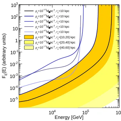
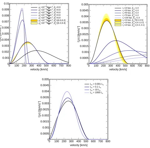
E F -5 10 -4 10 -3 10 -2 10 -1 10 1 10 2 10 3 10 =10 kpc s , r -3 pc M -1.0 =10 s ρ =10 kpc s , r -3 pc M -1.5 =10 s ρ =10 kpc s , r -3 pc M -2.5 =10 s ρ =10 kpc s , r -3 pc M -3.5 =10 s ρ =10 kpc s , r -3 pc M -4.5 =10 s ρ =[10,20] kpc s , r -3 pc M -1.5 =10 s ρ =[20,40] kpc s , r -3 pc M -1.5 =10 s ρ =[40,60] kpc s , r -3 pc M -1.5 =10 s ρ

FIG. 2. The energy-dependent part of the phase-space density (in arbitrary units). Different shades of blue indicate the dependence onρs for fixed rs (the baryonic components of the mass model and the L-dependent part of the phase-space density are also fixed). The yellow bands show how FE(E) changes whenρsis kept constant and rsis varied.

and f1(v) turns out to be much less dependent on the form of

FL(L) than FE(E), and therefore it is possible to reconstruct f1(v) with reasonable uncertainties even when marginalizing overβ0,β∞and L0.

Fig. 2 shows how FE(E) depends on the gravitational

po-tential of the system once the parameters entering in FL(L) are

fixed. We only consider the effect of changing the character-istic density,ρs, and the scale radius, rs, of the DM halo. For a given value of rs, decreasingρscorresponds to decreasing the amount of DM present in the halo and therefore the max-imum value of the gravitational potential (i.e. the value at the center of the MW). This is why on decreasing the characteris-tic density, the range of E values over which FE(E) is defined

becomes smaller. Forρs below approximately 10−1.5M⊙pc−3

the baryonic component becomes important in particular for the largest values of energy, which correspond to the central region of the halo. Once the inner potential is dominated by baryons, the behaviour of FE(E) at high energies is

indepen-dent ofρs and the only remaining effect is at low energies, where FE(E) decreases as ρs is decreased, simply because there is less DM.

The yellow bands show the behaviour of FE(E) as the scale

radius is varied, withρskept constant. Increasing rsleads to an increase in the amount of DM in the MW and therefore

FE(E) moves to larger values.

char-velocity [km/s]

0 100 200 300 400 500 600 700 800

]

-1

(v) [(km/s)1

f 0 0.001 0.002 0.003 0.004 0.005 0.006 0.007 0.008 0.009 0.01 =0.0 0 β , -3 pc M -1.0 =10 s ρ =0.0 0 β , -3 pc M -1.5 =10 s ρ =0.0 0 β , -3 pc M -2.5 =10 s ρ =0.0 0 β , -3 pc M -3.5 =10 s ρ =0.0 0 β , -3 pc M -4.5 =10 s ρ =[0.0,0.2] 0 β , -3 pc M -1.5 =10 s ρ =[0.2,0.4] 0 β , -3 pc M -1.5 =10 s ρ velocity [km/s]

0 100 200 300 400 500 600 700 800

]

-1

(v) [(km/s)1

f 0 0.0005 0.001 0.0015 0.002 0.0025 0.003 0.0035 0.004 0.0045 0.005 =1.0 inf β =10 kpc, s r =1.0 inf β =20 kpc, s r =1.0 inf β =40 kpc, s r =1.0 inf β =70 kpc, s r =1.0 inf β =100 kpc, s r =[0.2,0.5] inf β =10 kpc, s r =[-0.1,0.2] inf β =10 kpc, s r =[-0.4,-0.1] inf β =10 kpc, s r velocity [km/s]

0 100 200 300 400 500 600 700 800

]

-1

(v) [(km/s)1

f 0 0.0005 0.001 0.0015 0.002 0.0025 0.003 0.0035 0.004 0.0045 0.005 s

= 0.001 L

0

L

s

= 0.1 L

0

L

s

= 10 L

0

L

s

= 1000 L

0

L

FIG. 3. Upper left panel: the f1(v) distribution for various values ofρs(all other parameters are left unchanged). The yellow bands show the effect of changingβ0. Upper right panel: the same as the left panel but for the dependence on the scale radius (lines) and onβ_∞(bands). Lower panel: the same as the upper panels but for the dependence on L0. Note that the lines corresponding to L0=10 Lsand L0=1000 Lscoincide.

acteristic density is increased the range within which f1(v) is non zero gets larger and, therefore, the peak of the distribu-tion is reduced since f1(v) is normalized to one. As in Fig. 2, increasing the scale radius (withρsfixed) increases the grav-itational potential and the escape velocity, and therefore the peak in the speed distribution moves to higher speeds.

The yellow bands show the effect of changingβ0 andβ∞.

The effect is small and is localized at small/intermediate (in-termediate/large) velocities for β0 (β∞). Note that the

grav-itational potential is fixed and therefore picking one specific

velocity completely determines the energy of the DM parti-cle. Small velocities correspond to large energies (remember that E = Φ(x_⊙)₋v2/2) and to orbits localized close to the center of the halo. On the other hand, particles with large ve-locities will have small energies and will move on orbits that can reach large distances. Therefore the low (high)-velocity regime changes more asβ0(β∞) is varied.

reason when the transition happens more or less at R0, the ef-fect of increasing L0is the same as increasingβ∞. Finally, for

large L0, the velocity distribution becomes independent of L0 since increasing the transition scale only affects large radii.

The ranges we take for the parameters defining FL(L) in

Fig. 3 approximately match the ranges over which we carry out our scans (see Tab. I). The anisotropy at the center is con-strained to be smaller than half the central slope of the DM halo profile [111]. This imposes an upper limit of 0.5 for the case of a NFW halo and only allows zero or negativeβ0 for Einasto and Burkert profiles. However the halos formed in

N-body simulations do not have negativeβ0, and therefore we only considerβ0 ≥ −0.5. We allowβ∞to vary between -0.5

and 1.0, allowing for the possibility ofβ_∞< β0.

V. RESULTS AND DISCUSSION

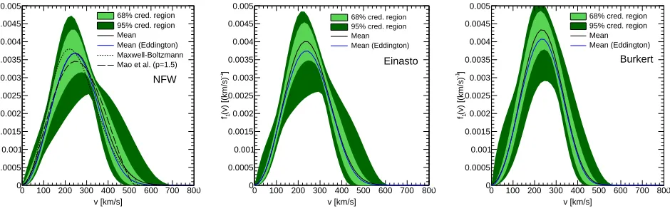
In this section we present our results for the probability dis-tribution of the speed disdis-tribution f1(v), derived from the scans discussed in Sec. III. In Fig. 4, f1(v) is obtained through the Eddington formalism, assuming isotropy. The light (dark) blue bands show the 68% (95%) credible interval and the solid black line corresponds to the mean. The distribution is recon-structed with an uncertainty of a factor of 2 (at 68% credible interval) for speeds smaller than 500 km s−1. This is consis-tent with the results of Refs. [13, 33]. There seems to be a characteristic speed (around 300 km s−1) for which the speed distribution has a minimum uncertainty. This is particularly evident for the case of a NFW halo. We believe this is just a consequence of imposing the normalization of f1(v) to 1. Dif-ferent mass models in the scan correspond to different gravita-tional potentials and, thus, to more peaked or extended speed distributions (see Fig. 3). However, increasing the amplitude of the peak has to lead to a less populated high-speed tail and, therefore, to a transition speed where smaller changes are ob-served7_.

Our main result is displayed in Fig. 5 where we show the probability distribution of f1(v) obtained through the proce-dure summarized in the previous section (i.e. introducing a three-parameter form for FL(L), deriving FE(E) in a

self-consistent way and marginalizing over the three parameters). As in Fig. 4, the light (dark) green shows the uncertainty in the reconstruction by means of the 68% (95%) credible interval and the solid black line corresponds to the mean. As expected, the reconstruction is worse than the isotropic case in Fig. 4, due to the presence of the three parameters in FL(L), however

the speed distribution can still be determined with an accu-racy of a factor of 4-5 for velocities smaller than 500 km s−1. The most uncertain part is, as before, the high-speed tail. The region of small uncertainty at around 300 km s−1 is more ev-ident than in the isotropic case and an additional region with

7_{Note that, even if each f}

1(v) (corresponding to a specific mass models) has to be normalized to 1, the mean in Fig. 4 (and in Fig. 5) does not necessarily integrate to 1, since it does not correspond to a specific mass model.

small uncertainty appears at around 100 km s−1. These re-gions could already partially be seen in Fig. 3. The region at smaller (larger) speeds results from the effect of changingβ0 (β_∞)8_.

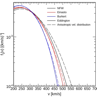
The solid blue lines show the speed distribution obtained through the Eddington formalism as in Fig. 4. For a more physical comparison the two distributions should be normal-ized to the same value, and once that is done the difference is small. For all of the DM halo profiles considered the tail of the speed distribution, beyond_∼500 km s−1, is larger in the anisotropic case, and consequently the peak of the distribution is lower. The effect is approximately a factor of 2 for the NFW halo, while it is less pronounced for the Einasto and Burkert halos (see Fig. 6). This is probably due to the marginalization overβ_∞and the uncertainty in the behaviour of the DM halo at large radii.

In the left panel of Fig. 5, for the case of the NFW halo, we also compare our results to the velocity distribution of the SHM (black dotted line) and the parametrization proposed by Mao et al. in Refs. [112, 113] as a fit to the results of N-body simulations. This parameterization also provides a good fit to the DM speed distribution found in a hydrodynamical simula-tion of a MW-like galaxy containing baryons [107]. In each case the circular and escape speeds are set to the mean values from Tab. II and we set p, which parameterizes the shape of the high speed cut-off, to 1.5 as suggested by [113]. As al-ready pointed out in Ref. [112], the self-consistent isotropic

f1(v) has a lower high-velocity tail (solid blue line) than the Mao et al. phenomenological parameterization (dashed black line in the upper left panel of Fig. 5). Our self-consistent anisotropic distribution (solid black) is however close to the Mao et al. parameterization (dashed black), which lies inside our 68% credible band.

VI. SUMMARY AND CONCLUSIONS

In this paper we developed a mass model for the MW, with the goal of studying the local DM velocity distribution in the case of a DM halo with an anisotropic velocity tensor.

Our MW mass model, inspired by Refs. [11, 15], assumes that the matter density of our own Galaxy can be written as a sum of four components: a disk, a combination of bulge and bar, a gaseous component and a DM halo. The free parameters entering in the modelling of these components are constrained by imposing a large set of astronomical observations (includ-ing the measurement of the proper motion of Sgr A∗, the local surface density and terminal velocities, as well as information derived from the motion of masers and halo stars and from microlensing).

Such observations constrain the gravitational potential of the MW from which it is possible to reconstruct the DM phase-space density F(E) (via the Eddington equation), under

8_{Following the discussion given before, changing L}