warwick.ac.uk/lib-publications
Original citation:He, Wei, Luo, Xing, Kiselychnyk, Oleh, Wang, Jihong and Shaheed, Mohammad Hasan. (2016) Maximum power point tracking (MPPT) control of pressure retarded osmosis (PRO) salinity power plant : development and comparison of different techniques. Desalination, 389 . pp. 187-196.
Permanent WRAP URL:
http://wrap.warwick.ac.uk/78938
Copyright and reuse:
The Warwick Research Archive Portal (WRAP) makes this work by researchers of the University of Warwick available open access under the following conditions. Copyright © and all moral rights to the version of the paper presented here belong to the individual author(s) and/or other copyright owners. To the extent reasonable and practicable the material made available in WRAP has been checked for eligibility before being made available.
Copies of full items can be used for personal research or study, educational, or not-for-profit purposes without prior permission or charge. Provided that the authors, title and full bibliographic details are credited, a hyperlink and/or URL is given for the original metadata page and the content is not changed in any way.
Publisher’s statement:
© 2016, Elsevier. Licensed under the Creative Commons Attribution-NonCommercial-NoDerivatives 4.0 International http://creativecommons.org/licenses/by-nc-nd/4.0/
A note on versions:
The version presented here may differ from the published version or, version of record, if you wish to cite this item you are advised to consult the publisher’s version. Please see the ‘permanent WRAP url’ above for details on accessing the published version and note that access may require a subscription.
Maximum power point tracking (MPPT) control of pressure retarded osmosis (PRO) salinity power plant: development and comparison of different techniques
Wei He a, b,*, Xing Luo a, Oleh Kiselychnyk a, Jihong Wang a, Mohammad Hasan Shaheed b,*
a School of Engineering, University of Warwick, Coventry, CV4 7AL, UK
b School of Engineering and Material Science, Queen Mary University of London, London, E1 4NS, UK
Abstract:
This paper presents two new methods for the maximum power point tracking (MPPT) control of a pressure retarded osmosis (PRO) salinity power plant, including mass feedback control (MFC) and fuzzy logic control (FLC). First, a brief overview of perturb & observe (P&O) and incremental mass resistance (IMR) control is given as those two methods have already demonstrated their merit in good control performance. Then, two new methods employing variable-step strategy, MFC and FLC, are proposed to address the trade-off relationship between rise-time and oscillation of P&O and IMR. Genetic Algorithm (GA) is used for finding the optimum parameters of membership functions of FLC. From the case-study of start-up of the PRO adopting MPPT control, MFC and FLC have shown faster convergence to the target performance without oscillation compared with P&O and IMR. These four MPPT techniques are further evaluated in case-studies of state transitions of the PRO due to operational fluctuations. It is proven that the MPPT using FLC and modified MFC has better performance than the other two methods. Finally, the paper reports a comparison of major characteristics of the four MPPT methods, which could be considered as guidance for selecting a MPPT technique for the PRO in practice.
Keywords: Pressure retarded osmosis, Maximum power point tracking, Mass feedback control, Fuzzy logic control, Genetic algorithm
*Corresponding author: Tel: + 44(0)20 7882 3774(W He), +44 (0)20 7882 3319(MH Shaheed)
1. Introduction
Pressure retarded osmosis (PRO) is a promising method which is potentially capable of producing power and processing water simultaneously because of its nature of combination of the water treatment and renewable energy generation. In other words, it can be used as not only a clean energy generator, but also a water treatment to recycle water. In a PRO plant, chemical potential between the two salinities is converted to hydraulic potential which is harvested using hydro-turbines. The energy conversion and the water recycle are based on the transportation of the pure water from the low concentration side to the high concentration side, due to the higher osmotic pressure difference across the membrane than the hydraulic pressure applied on the draw solution.
Generation of salinity power, or osmotic power, using PRO has been widely investigated in the last five years. It is reported that the economic viability can be achieved if the power density is higher than 5 W/m2 [1]. The commercial reverse osmosis (RO) membranes and forward osmosis (FO)
membranes are inappropriate for the PRO applications because of different operational conditions. The bulky support layers of the RO membranes cause severe internal concentration polarization (ICP) and significant decrease in water flux. In contrast, the highly open substrate of the FO membranes does not possess the sufficient mechanical strength to withstand the pressure applied in the PRO process. Therefore, in order to realise the PRO process in practice, first, specific high performance membranes for the PRO process have been investigated. Recently, Li et al. developed a TFC polyetherimide PRO flat–sheet membrane which is able to maintain almost unchanged water flux and power density of 12.8 W/m2 at 17.2 bar over 10 hours [2]. While maintaining a relatively small
structural parameter to minimize ICP, enhancing membrane water permeability during the formation of polyamide layers and/or novel post-treatment is also important [3]. Cui et al. optimized the interfacial polymerization reaction and alternative post-treatments, and fabricated a membrane with power density of 18.09 W/m2 at 22 bar when using 1 M NaCl as draw solution and DI water as
feed [4]. A comprehensive review of the development of the high performance PRO membranes can be found in [3].
The process characteristics of the PRO and the optimization of the configuration and operation are the second step to develop practical applications taking advantages of the fabricated high performance membranes. Compared to the lab-scale PRO process, mass transfer of the water and salts across the membrane is highly affected by the increasing membrane usage and the hydrodynamic flows of the salinities. It is reported that although the total extractable energy capacity of the PRO is enhanced with the increase of the membrane area, the average membrane power density is significantly decreased due to the rapidly vanishing net driving force [5]. Sivertsen et al. constructed an iso-watt diagram of PRO as a map to link the membrane properties and the lab-scale membrane performance [6]. Furthermore, He et al. constructed an operation map of the lab- scale-up PRO process to identify the coscale-upled effects of the increased process scale with the membrane properties [7]. These operation maps nicely illustrated the characteristics of the PRO from lab-scale to the scale of practical applications. Moreover, to mitigate the detrimental effects of ICP, external concentration polarization (ECP) and reverse solute permeation (RSP), different configurations have been studied to enhance the overall performance of the system. Hybrid RO-PRO is one of the widely investigated configuration due to the inherently benefiting performance of the two processes [8]. Achilli et al. carried out both numerical and experimental investigations on the hybrid RO-PRO plant [9, 10]. The maximum power density of PRO can be approximately achieved up to 10 W/m2 in the
carried out systematic modelling and optimization of dual-stage PRO process [11-14] and hybrid FO/RO/PRO process [15, 16]. PRO also shows promising performance in other hybrid processes. In a novel PRO-MD (membrane distillation) hybrid process, the maximum power densities of 31.0 W/m2
and 9.3 W/m2 by the PRO using DI water and real wastewater mixing with 2M NaCl concentrate [17].
In another hybrid multi-stage vacuum MD and PRO process, maximum power density of 9.7 W/m2 is
achieved when river water is used as feed solution [18]. Recently, a preliminary investigation of hybrid photovoltaic (PV) solar and PRO osmotic energy has been proposed and studied. The demonstrated benefiting improvements of both renewable energy generation and water desalination especially push the osmotic power to the market [19].
Accordingly, based on the significantly improved membrane performance and the increasingly clear understanding of the process characteristics of the scale-up PRO, another key step to push the technology realisation in practical applications is control of input variables of the PRO, such as hydraulic pressure applied on the draw solution, to ensure the optimized performance. In fact, studies focusing on optimal control have been important topics of research in solar, wind, wave, tidal, and other renewable energy generations. But due to the difficulty of deriving the analytical solutions for complex systems, the stable, robust and efficient maximum power point tracking (MPPT) systems represent a challenge for renewable energy designers. MPPT is used to operate the renewable energy generators in a manner to maximize the output power, irrespective of the operational fluctuations and variations. According to the significant development in last decades, several algorithms have been developed in tracking the maximum power point (MPP) for not only solar PV arrays [20-26] but also for fuel cell power plant [27, 28]. In this context, in order to maximize the performance of PRO in practice, MPPT controller is essential to ensure the design operation and performance of a PRO power plant. However, at the early stage of studying the MPPT in PRO, there is very limited work reported in the literatures. In our previous study, two algorithms for MPPT in a PRO are proposed and investigated, including perturb & observe (P&O) algorithm and incremental mass resistance (IMR) algorithm [29]. It is demonstrated by simulations that both P&O and IMR algorithms can be used to track the MPP of a PRO process at the steady-state operations and the transiting operations due to the operational fluctuations. But the trade-off between the rise time and the oscillation by selecting the step-size of the perturbation pressure or incremental pressure exists in both algorithms. Larger step-size results in fast response as well as larger oscillation, and vice versa.
Therefore, in this study, in order to balance the trade-off relationship between the rise-time and oscillation, two new MPPT controllers, mass feedback control (MFC) and fuzzy logic control (FLC), are developed and compared with P&O and IMR methods. First, the four methods are introduced, in which algorithms of MFC and FLC are described in details. For the MPPT using FLC, genetic algorithm (GA) is used to search for the optimum parameters for the settings of the membership functions. Then, two case studies are carried out to evaluate the two new MPPT controllers and compare the four algorithms. Finally, as guidance for the designers and users to select a MPPT algorithm for a particular PRO application, a table that summaries the major characteristics of the methods is also provided.
2. Process characteristics of a PRO salinity power plant
Fig. 1 shows the characteristic power curve for a scale-up PRO plant. The problem considered by MPPT techniques is to automatically find the applied pressure (PMPP) at which a PRO power plant
to the fluctuations of the operations, such as temperature, pressure and flow conditions, the MPP also varies. Therefore, the MPPT controller is required not only to fast reach the MPP at the start-up process but also automatically respond to changes in the process due to operation fluctuations. Moreover, once the MPP is found, a smooth operation with insignificant oscillation needs to be maintained by the MPPT controller.
Figure 1 Characteristic PRO power curve.
3. MPPT control
The four MPPT control algorithms considered in this study are introduced in this section, including two previously developed methods in [29], P&O and IMR, and two new methods, MFC and FLC. P&O and IMR are briefly introduced below and details of the two algorithms can be found in [29].
3.1. Perturb & observe
[image:5.595.160.439.644.744.2]P&O involves a perturbation in the applied pressure on the draw solution to search for the MPP of the PRO salinity power generator. Incrementing (decrementing) the applied pressure increases (decreases) the power when operating on the left of the MPP and decreases (increases) the power when on the right of the MPP. Therefore, if the measured power is increasing at the sample instant, the subsequent perturbation should be kept the same to reach the MPP and if the measured power is decreasing, the perturbation should be reversed. The P&O based MPPT method is summarised in Table 1. The P&O process is repeated based on the algorithm until the MPP is reached. Due to the perturbation size, an oscillation is always accompanied. A larger perturbation pressure leads to fast convergence but a larger oscillation as well. In contrast, a smaller perturbation pressure slows down the MPPT.
Table 1 Direction of pressure perturbation of P&O.
Change in power
Perturbation Pressure
Positive Negative
Positive Positive Negative
3.2. Incremental mass resistance
IMR is based on the fact that the slope of the PRO power curve is zero at the MPP, positive on the left of the MPP, and negative on the right, as given by
/ 0, at MPP
/ 0, left of MPP
/ 0, right of MPP
dW dP
dW dP
dW dP
(1)
Because of the slope of the PRO power curve can be also approximated by the incremental pressure, pressure, flow rate and the flow rate change, which is presented as,
( ) 1 1
( ) ( )
M M M
dW d PV dV V
V P V P
dP A dP A dP A P (2)
where V presents the volumetric flow rate. With a fixed membrane area, equation (1) can be rewritten as
/ / V or / / P , at MPP
/ / V or / / P, left of MPP / / V or / / P, right of MPP
P V P V P V
P V P V P V
P V P V P V
(3)
where /P V and P/ V are defined as the instantaneous mass resistance and the incremental mass resistance, respectively. Mass resistance refers to the difficulty to pass a particular flow rate of the permeation through the membrane in a PRO. The inverse quantity of the resistance is mass conductance, describing the ease with which a current of the permeation passes. Therefore, the MPP can be tracked by either comparing the instantaneous mass resistance ( / VP ) to the incremental mass resistance ( P/ V) or comparing the instantaneous mass conductance ( /V P )
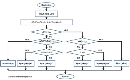
to the incremental mass conductance (V/P), as shown in equation (3). In fact, the two comparisons are equivalent in mathematics and mass resistance, namely IMR, is selected in this study to calculate the slope of the PRO power curve. A flowchart of the algorithm is shown in Fig. 2. On one hand, similar to the P&O algorithm, the incremental pressure determines the convergence of the MPPT. Fast tracking can be achieved with larger increments but accompanying with an oscillation. Therefore, how to select the incremental pressure is a trade-off to balance the convergence and oscillation. On the other hand, control parameter in IMR,
IMR, can be used toFigure 2 Flowchart of IMR algorithm. C is value of the step pressure.
3.3. Mass feedback controller
With DSP and microcontroller which are capable to handle complex computation, an obvious way of performing MPPT is to compute the slope of PRO power curve (dW dP ) and feed it back to / the step-pressure at the next sample instant to drive it to zero. The way to compute the slope and feedback is determined by the user. Inspired by the conventional PI control which attempts to minimize the error over time by adjustment of a control variable, a PI-like mass feedback control (MFC) is also proposed in this section. The aim of MFC is to minimize the slope of the PRO power curve over time by adjusting the step-pressure. Therefore, the algorithm below is used for MFC,
1
( ) p[( )n ( )n ] i( )n
dW dW dW
P n k k
dP dP dP
(4)
where k , and p ki both non-negative, denote the coefficients for the proportional and integral gains,
respectively. Unlike IMR algorithm that use only the sign of the slope, MFC effectuates an adaptive gain that the fast convergence achieves, the further the position of the actual operation point is from the MPP. In the proposed MFC, the step-pressure is the sum of two terms: the first term is proportional to the change of the slope and the second term is proportional to the slope.
3.4. Fuzzy logic control
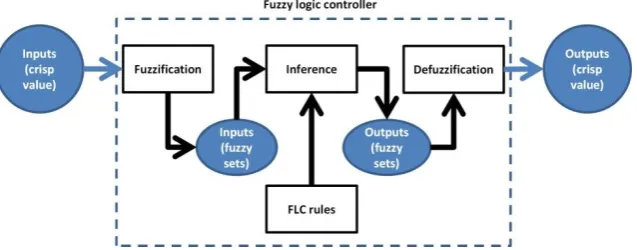
non-linearity. Generally, as depicted in Fig. 3, a FLC normally consists of four main steps/components: 1) Fuzzification. A fuzzifier is designed to map crisp values of the inputs into fuzzy sets to activate rules; 2) FLC rules. The rules are defined to design the FLC behaviour by using a set of IF-THEN statements of the FLC rules; 3) Inference. Based on the rules, the inference engine maps the input fuzzy sets into output fuzzy sets; 4) Defuzzification. A defuzzifier is applied to map output fuzzy sets into crisp values.
Figure 3 Block diagram of the fuzzy logic control
The rules are the key components to determine the FLC operation, which is expressed as linguistic variables in terms of fuzzy sets. The output is obtained by applying an inference mechanism, which includes [30]: membership functions, connections linking the rules antecedents, implication function and rule aggregation operator. The membership functions are usually piece-wise linear function associated to the FLC linguistic variables, such as triangular or trapezoidal functions. The number and the shape of the membership functions of each fuzzy set as well as fuzzy logic inference mechanism are selected by the operators and thus the performance of the FLC depends on the experiences of the designers. The searching rules formulation in this work is based on the PRO power curve as shown in Fig. 1. If the last change in the applied pressure causes the power to rise, keep searching in the same direction; otherwise, if the last change causes the power to drop, move to the opposite direction.
The FLC control is achieved based on satisfaction of two criteria relating two input variables, namely slope and change of slope, at a particular sampling instant. Similar to the error and the change of the error in the conventional FLC, the controller drives these two variables to zeros when the steady-state MPP is reached. Therefore, at the sampling instant n, the two variables, slope (E) and change of slope (E) are expressed as
( ) ( 1)
( )
( ) ( 1)
W n W n E n
P n P n
(5)
( ) ( ) ( 1)
E n E n E n
(6)
trapezoidal-shaped membership function is selected for fuzzy sets of NB and PB, and triangular-shaped membership function is selected for fuzzy sets of NS, ZE and PS. The parameters of these membership functions are based on the range of values of the numerical variables.
Figure 4 Illustrated membership functions of the input variables, E and ΔE, and the output variable, ΔP.
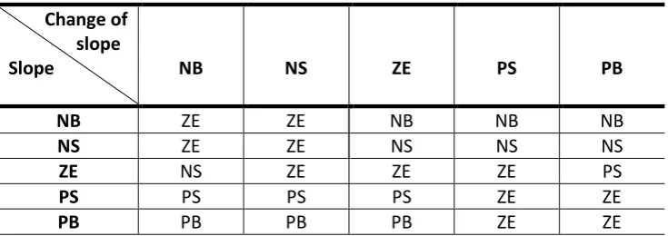
The pre-defined rules are important to determine the output step-pressure subject to different operations. The look up table of the rules used in this study is shown in Table 2, in which the linguistic variables assigned to step-pressure for the different combinations of the slope and the change of the slope are based on the knowledge and experiences of the users. As shown in the table, for example, the operating point is far to the left of the MPP, that the slope is PB, and the change of the slope is ZE, then a relatively large positive perturbation pressure should be added that is perturbation pressure should be PB to reach the MPP.
Table 2 Fuzzy rule based look up table.
Change of slope
Slope NB NS ZE PS PB
NB ZE ZE NB NB NB
NS ZE ZE NS NS NS
ZE NS ZE ZE ZE PS
PS PS PS PS ZE ZE
PB PB PB PB ZE ZE
[image:9.595.115.483.503.633.2]2
2 2
1
( MPP ) N ( MPP (n))
n
f
e dt
W W dt
W W (7)where W is the average power output, WMPP is the MPP at the selected operation condition, and
N
is number of selected sample instants in optimization. In the future applications, the reference operation should be the design operation or the standard operation of a particular PRO power plant. In this study, the reference MPP is selected the steady-state MPP found by the MPPT using P&O. Number of sample instants to reach the MPP using P&O and IMR at the start-up process is varied with different perturbation pressure or incremental pressure [29]. The number of sample instants to reach the MPP using P&O is approximately between 5 to 20 in the start-up process using perturbation pressure of 5, 1, 0.5 bar from the initial pressure 1 bar [29]. Therefore, 20 sample instants are considered in the fitness function.In order to improve the FLC performance, parameters of all the variables are optimized using GA. GA optimization employs the concepts of evolutionary theory, and provide an effective search in a large and complex solution space to obtain the optimum solutions. The algorithm is also known for avoiding local minima than gradient based algorithm. To use GA, parameters to be optimized need to be translated into chromosomes of an individual. Then a population of individuals which represent different possible parameters of variables to the minimization of the fitness function is evolved toward better design of FLC. Therefore, the population of GA optimization consists of a set of individuals, each of which has three chromosomes representing E, E and P. Because the same structure of membership functions are selected for inputs and output as shown in Fig. 4 in this study, chromosome uses the same presentation for all the three variables. Generally, the chromosome can be different to represent different designs of the membership functions of a variable to be optimized.
The five membership functions as shown in Fig. 4 can be expressed by six parameters including four parameters presenting the distances ( i1
k C , i2
k
C and o k
C ), the minimum (lminj ) and the maximum
( max
j
l ). Therefore, an individual is composed of eighteen parameters which are illustrated in Fig. 5.
The relation between C , ki1
2
i k
C and C (ko k1,2,3,4) and coordinates of the membership functions of
the three variables, i1
k x , i2
k
x and o k
x are respectively given [30],
1 4 3 min
2 3 min
3 2 max
4 1 2 max
( )
( )
j j j j
j j j
j j j
j j j j x C C l x C l x C l x C C l
(8)
where j presents the first input variables (i1) E, the second input variable (i2) E and the output variable (o) P. The parameters of i1
k C , i2
k
C and o k
C (k1,2,3,4) are restricted and the minimums and maximums are determined by the users [30]. In this study, they are:
1 2 1 2
min min max max
min max
1 2
0.3 , 0; 0 , 0.3;
15 0; 0 15;
0 , , 1, k=1,2,3,4
i i i i
o o
i i o k k k
l l l l
l l
C C C
Figure 5 An illustrated individual used in GA optimization.
Therefore, based on equations (8), membership functions of the three variables can be represented by an individual in the population.
Moreover, with the defined individuals and fitness function, the optimization can be carried out. In GA, first an initial population is generated. A set of chromosomes should be randomly chosen to ensure the diversity of the solution candidates at the beginning. Then, GA uses the operations of selection, crossover and mutation to generate next generation. When the maximum value of the fitness functions is achieved with respect to a pre-defined value, the optimization is terminated. Otherwise, the optimization is working from generation to generation. In this study, the GA optimization is achieved using GA optimization toolbox of MATLAB. A population with 100 individuals has been taken to search for the optimum parameters. For the selection, the fitness function is set as equation (7). Selection function is stochastic uniform (selectionstochunif), in which each parent is chosen depending on a section of the line of length proportional to its scaled fitness value. Crossover fraction (CrossoverFraction) is used, which specifies the fraction of the next generation other than elite scheme. In order to make sure the coordinates 1
j
x and 4
j
x within the
predefined range, a set of linear constraints are used for all variables, which are C1j C2j 1 and
3 4 1
j j
C C . And the upper and lower bounds for the parameters are set based on equation (9). According to the optimization toolbox, when the problem has linear/bound constraints, the mutation function mutationadaptfeasible is used. The settings of the toolbox are: Crossover fraction of each population 0.7, mutation fraction 0.3, and TolFun (tolerance of function), which is the average change of fitness function between two consecutive iterations and used as the stop criterion, 1×10⁻¹⁰.
4. Evaluation and comparison of MPPT controllers 4.1. MPPT of a PRO salinity power generator
by a fast and stable controller. Current literatures suggested that the transition from one steady state to another steady state for RO process changes in different applications. Bartman et al. altered the flow rate less than ~1 min within a wide range of operation in UCLA experimental RO membrane water desalination system [33]. Sassi et al. reported that pseudo steady-state model of RO can be considered for time-step more than 0.25 h [34]. For PRO, currently there is no reported literature studying the transition between the operations. But due to the inherent similarity to RO desalination plant, the range of the transition time can be estimated. In this study, a general sample instant is used for representing the sensing period [29]. The sample instant is assumed to be larger than the transition time caused by applying the step pressure.
Figure 6 An illustrated PRO power plant using MPPT.
4.2. Case study of MPPT: start-up of a PRO salinity power generator
The parameters used in this section are shown in Table 3. The performance of the PRO salinity power generator is obtained based on the models and modelling framework developed in our previous work [35], which are described in Appendix A.1. The simulations in this study are under the following assumptions: i) osmotic pressure is considered to be linearly proportional to the concentration difference based on the modified van’t Hoff law [36]. In the salinity range of 0-70 g/kg, the modified linear osmotic pressure approximation is validated and the maximum deviation is 6.8% [36, 37]; ii) constant hydraulic pressure difference in the membrane channel due to the negligible pressure loss; iii) significant membrane fouling and deformation do not occur; iv) For simplicity, a constant density of the water is used for both draw and feed solutions [38].
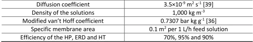
Table 3 Parameters used in the simulations of start-up of the PRO using MPPT controllers.
Parameter Value
Concentration of the draw solution 35 g/kg
Concentration of the feed solution 0.1 g/kg
Dimensionless flow rate 0.5
Temperature 298 K
Membrane water permeability coefficient 1.06×10⁻⁷ m·bar-1·s-1 [39]
Membrane salt permeability coefficient 2.62×10⁻⁸ m·s-1 [39]
Membrane structural parameter 4.62×10⁻³ m [39]
[image:12.595.90.508.629.762.2]Diffusion coefficient 3.5×10⁻⁹ m2 s-1 [39]
Density of the solutions 1,000 kg m-3
Modified van’t Hoff coefficient 0.7307 bar kg g-1 [36]
Specific membrane area 0.1 m2 per 1 L/h feed solution
Efficiency of the HP, ERD and HT 70%, 95% and 90%
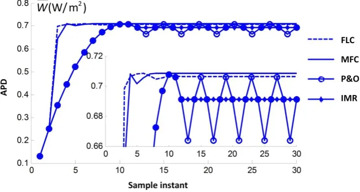
[image:13.595.83.510.73.144.2]The MPPT with the four algorithms are studied in the start-up of a PRO plant. The parameters used in P&O, IMR and MFC are listed in Table 4. For the FLC based MPPT, the parameters of the membership functions of both the inputs and output are optimized by GA. The optimized membership functions are shown in Fig. 7. FLC is implemented using MATLAB fuzzy logic toolbox. The results of the power outputs using the four MPPT controllers are shown in Fig. 8. For all the MPPT controllers, the initial pressure applied on the draw solution is 1 bar and the step-pressure (including both perturbation pressure and incremental pressure) are set to be 1 bar at the first sample instant.
Table 4 Parameters of P&O, IMR and MFC.
P&O IMR MFC
Perturbation pressure
1 bar Incremental
pressure
1 bar k p 140
2 2 bar m /W
IMR
1×10⁻³ bar or m3/sor m3 s-1 bar-1 ki 20
Figure 7 Optimized membership functions of the three variables.
According to the results shown in Fig. 8, obviously the performance of the MPPT is significantly improved using MFC and FLC compared to that using P&O and IMR. These two controllers, FLC and MFC, are faster to reach the MPP during the start-up, and present also a much smoother signal with less fluctuation in the quasi-steady state compared to P&O. Furthermore, although IMR has better performance than P&O, using the parameter
IMR toFigure 8 Power output with MPPT using P&O, IMR, MFC and FLC.
4.3. Case study of MPPT: operational fluctuations of a PRO salinity power generator
Furthermore, another case study of the MPPT controllers is presented at the operations subject to the fluctuations of the PRO plant. In fact, the PRO operation might be affected by many factors, such as temperature and applied pressure. Anastasio et al. reported that the permeability coefficients of water and solute increase from 0.589 L/(m2·bar·h) and 0.319 L/(m2·h) to 1.12
L/(m2·bar·h) and 0.580 L/(m2·h) respectively, when the temperature of the draw solution increases
from 20 0C to 40 0C [40]. It also has been reported that the high pressure induced the varied
Table 5 Varied parameters of solution characteristics and hydrodynamics and membrane properties [39]. The draw
solution studied is 35 g/kg (0.6 M approximately) NaCl solution.
Temperature (0C)
A ( -1 -1
m s bar )
B
( -1
m s )
D
( 2 -1
m s )
km
( -1
m s )
ICP factor, S/D
( 1 1
m s )
20 1.06×10⁻⁷ 2.62×10⁻⁸ 3.50×10⁻⁹ 4.27×10⁻⁴ 1.32×10⁶
30 1.43×10⁻⁷ 4.25×10⁻⁸ 4.54×10⁻⁹ 9.74×10⁻⁴ 1.00×10⁶
40 1.74×10⁻⁷ 5.87×10⁻⁸ 5.74×10⁻⁹ 10.88×10⁻⁴ 0.82×10⁶
50 1.98×10⁻⁷ 8.00×10⁻⁸ 7.09×10⁻⁹ 11.98×10⁻⁴ 0.71×10⁶
Based on the parameters as listed in Table 5, a series of tests are carried out to compare the four MPPT algorithms. The simulations are performed using a changing temperature profile as shown in Fig. 9. Generally, the operating temperature changes gradually in practice. For testing the controllers, simulations are carried out considering the operational temperature changes instantly, which is more difficult for MPPT to track the suddenly changed MPP. Specifically, we consider a 175 sample instants time window in which the temperature is varied. At the end of every 25 sample instants, the temperature increases or decreases by o
10 C. The parameters and settings are same to those of the tuned MPPT controllers in the case study of the start-up. According to the simulations, the tuned MFC (tuned parameters listed in Table 3) in the case study of start-up does not have very good performance in the studied cases of state transition using parameters as shown in Table 5. A too large step pressure resulted from MFC at the 26th sample instant leads to significant decrease of
process performance from o
20 C to o
30 C at the 26th. A limitation of the step pressure can be added
in the MFC to avoid a too much step pressure caused by the suddenly changed operation. A simple scheme can be used to limit the step pressure, which is P(n) P0 if
P
(n)
calculated byequation (4) is larger than the limiting step pressure Pmax.
D
P
0 is the actuated step pressure andit can be controlled to change the performance of the MPPT but
D
P
0£
D
P
max should be considered.Figure 9 Power output of the PRO power plant using MPPT controllers of different algorithms subject to fluctuating
operational temperatures.
Moreover, another test of these four algorithms is carried out in the case study of the PRO power plant subject to fluctuating operational concentrations and flow rates, in which both the draw solution and the feed solution are considered. Specifically, we consider a 60 sample instants time window in which the concentrations of draw and feed, and the dimensionless flow rates are changed as shown in Fig. 10 (a), 10(b) and 10(c), respectively. The dimensionless flow rate is the ratio of the flow rate of the feed to the sum of the both flow rates, which is qF0/ (qD0qF0). As shown in Fig. (10),
Figure 10 Variations of salinities including concentrations of the draw shown in (a) and the feed shown in (b), and the
dimensionless flow rate shown in (c).
Figure 11 Power output of the PRO power plant using MPPT controllers of different algorithms subject to fluctuating
operational concentrations and flow rates.
4.4. Comparisons and discussions of MPPT controllers
Table 6 Major characteristics of the four MPPT controllers.
MPPT algorithm P&O IMR MFC FLC
PRO dependent? No No No No
Analog or Digital? Both Digital Digital Digital
Periodic tuning? No Varies Yes Yes
Convergence speed Varies Varies Fast Fast
Oscillation? Yes No No No
Implementation complexity Low Medium Medium High
Vulnerable to variable operations Low Low Medium Medium
5. Conclusion
In this study, two new MPPT controllers used in the PRO power plant are proposed and evaluated, including MFC and FLC. To optimize the performance of the MPPT using FLC algorithm, GA optimization is used to find the optimum parameters for the membership functions of both the input and output variables in FLC. Then, the four MPPT controllers are compared in selected case studies. One is the start-up of the PRO and the other is the fluctuating operated PRO due to the varied temperature and salinities. Finally, based on the comparisons, the major characteristics of these four methods are presented. Therefore, according to the results, some conclusions can be drawn: 1) using MPPT at the start-up of the PRO, compared to P&O and IMR algorithms, both MFC and FLC are capable to adaptively change the step-pressure to balance the trade-off relationship between the rise-time and the steady-state oscillation; 2) optimized FLC and modified MFC algorithm are capable to deal with the operational fluctuations. MPPTs using FLC and modified MFC have the better performance than the MPPTs using P&O and IMR algorithms, meaning faster convergence and lower oscillation during all the tested start-up and steady-state transitions; 3) the comparable table can be served as a useful guide in choosing the right MPPT algorithm for a specific PRO application.
Nomenclature
A Membrane water permeability [ -2 -1 -1
L m s bar ]
m
A Membrane area [ 2
m ]
B Membrane solute permeability [L m h -2 -1]
c Concentration of solution [kg kg -1]
k
C Generic parameters used for designing membership functions
OS
C Modified van’t Hoff law coefficient [bar kg g ] 1
D Diffusion coefficient [ 2 -1
m s ]
m
k Mass transfer coefficient [ -1
m s ]
W
J Water permeation flow rate [ -2 -1
L m h ]
S
J Reverse solute permeation flow rate [ -2 -1
L m h ]
min,max
l l Generic parameters presenting the minimum and the maximum of a
membership function
q Mass flow rate of solution [kg h -1]
S Membrane structure parameter [m]
V Volumetric flow rate of solution [ 3 -1
m h ]
W Average power density [W m -2]
x Generic parameters used for designing membership functions
Osmotic pressure [bar]
Dimensionless flow rate
Efficiency
Density of solution [kg m -3]Abbreviations
APD Average power density
BP Boost pump
ECP External concentration polarization
FLC Fuzzy logic control
HP High-pressure pump
HT Hydro-turbine
ICP Internal concentration polarization
IMR Incremental mass resistance
INC Incremental conductance
MFC Mass feedback control
MPP Maximum power point
MPPT Maximum power point tracking
NB Negative big
NS Negative small
PB Positive big
P&O Perturb & observe
PRO Pressure retarded osmosis
PS Positive small
PV Photovoltaic
RO Reverse osmosis
RSP Reverse solute permeation
TFC Thin-film composite
ZE Zero
Appendix: Mathematical model of a scale-up PRO salinity power generator
integrating the water flux and reverse salt flux. Then, update of salinities’ concentration and flow rate at each position in the flow channel can be done by equations (A.6), (A.7), (A.8) and (A.9). In order to evaluate the overall efficiency of the osmotic power extraction, average power density (APD) of a scale-up PRO is expressed by equation (A.11).
Table A.1 Mathematical model of a scale-up PRO plant.
Physical quantity Equation NO#
Water Flux exp( / ) exp( / )
( ( ) )
1 (exp( / ) exp( / ))
D W m F W
W os PRO
W W m
W
c J k c J S D
J A C P
B
J S D J k
J
(A.1)
Reverse salt flux exp( / ) Fexp( / )
B( )
1 (exp( / ) exp( / ))
D W m W
S
W W m
W
c J k c J S D
J
B
J S D J k
J
(A.2)
Power Density W J W PPRO (A.3)
Water Permeation d V( P)J d Aw ( m); qP
P VP (A.4)Reverse salt permeation d V( S)J d AS ( m);mS
S VS (A.5)Concentration of the draw 0 0
0
cD D S
D D P q m c q q (A.6)
Flow rate of the draw 0
D D P
q q q (A.7)
Concentration of the feed 0 0
F 0
c F S
F F P q m c q q (A.8)
Flow rate of the feed 0
F F P
q q q (A.9)
Average power density (APD)
0 PRO P F m P V W V A (A.10) Acknowledgments:
The authors would like to thank the funding support from Engineering and Physical Science Research Council (EPSRC), UK (EP/L014211/1 and EP/K002228/1). Wei He would like to thank the Henry-Lester Trust (UK) and the Great Britain–China Educational Trust (UK) for the generous sponsorship to his PhD project.
Reference:
[1] K. Gerstandt, K.V. Peinemann, S.E. Skilhagen, T. Thorsen, T. Holt, Membrane processes in energy supply for an osmotic power plant, Desalination, 224 (2008) 64-70.
[2] Y. Li, R. Wang, S. Qi, C. Tang, Structural stability and mass transfer properties of pressure retarded osmosis (PRO) membrane under high operating pressures, Journal of Membrane Science, 488 (2015) 143-153.
[4] Y. Cui, X.-Y. Liu, T.-S. Chung, Enhanced osmotic energy generation from salinity gradients by modifying thin film composite membranes, Chemical Engineering Journal, 242 (2014) 195-203. [5] W. He, Y. Wang, M.H. Shaheed, Energy and thermodynamic analysis of power generation using a natural salinity gradient based pressure retarded osmosis process, Desalination, 350 (2014) 86-94. [6] E. Sivertsen, T. Holt, W.R. Thelin, G. Brekke, Iso-watt diagrams for evaluation of membrane performance in pressure retarded osmosis, Journal of Membrane Science, 489 (2015) 299-307. [7] W. He, Y. Wang, I.M. Mujtaba, M.H. Shaheed, An evaluation of membrane properties and process characteristics of a scaled-up pressure retarded osmosis (PRO) process, Desalination, 378 (2016) 1-13.
[8] W. He, Y. Wang, A. Sharif, M.H. Shaheed, Thermodynamic analysis of a stand-alone reverse osmosis desalination system powered by pressure retarded osmosis, Desalination, 352 (2014) 27-37. [9] J.L. Prante, J.A. Ruskowitz, A.E. Childress, A. Achilli, RO-PRO desalination: An integrated low-energy approach to seawater desalination, Applied Energy, 120 (2014) 104-114.
[10] A. Achilli, J.L. Prante, N.T. Hancock, E.B. Maxwell, A.E. Childress, Experimental Results from RO-PRO: A Next Generation System for Low-Energy Desalination, Environmental Science & Technology, 48 (2014) 6437-6443.
[11] A. Altaee, A. Sharif, G. Zaragoza, Limitations of osmotic gradient resource and hydraulic pressure on the efficiency of dual stage PRO process, Renewable Energy, 83 (2015) 1234-1244.
[12] A. Altaee, A. Sharif, G. Zaragoza, N. Hilal, Dual stage PRO process for power generation from different feed resources, Desalination, 352 (2014) 118-127.
[13] A. Altaee, N. Hilal, Design optimization of high performance dual stage pressure retarded osmosis, Desalination, 355 (2015) 217-224.
[14] A. Altaee, N. Hilal, Dual stage PRO power generation from brackish water brine and wastewater effluent feeds, Desalination.
[15] A. Altaee, N. Hilal, Dual-stage forward osmosis/pressure retarded osmosis process for hypersaline solutions and fracking wastewater treatment, Desalination, 350 (2014) 79-85.
[16] A. Altaee, A. Sharif, G. Zaragoza, A.F. Ismail, Evaluation of FO-RO and PRO-RO designs for power generation and seawater desalination using impaired water feeds, Desalination, 368 (2015) 27-35. [17] G. Han, J. Zuo, C. Wan, T.-S. Chung, Hybrid pressure retarded osmosis-membrane distillation (PRO-MD) process for osmotic power and clean water generation, Environmental Science: Water Research & Technology, 1 (2015) 507-515.
[18] J.-G. Lee, Y.-D. Kim, S.-M. Shim, B.-G. Im, W.-S. Kim, Numerical study of a hybrid multi-stage vacuum membrane distillation and pressure-retarded osmosis system, Desalination, 363 (2015) 82-91.
[19] W. He, Y. Wang, M.H. Shaheed, Stand-alone seawater RO (reverse osmosis) desalination powered by PV (photovoltaic) and PRO (pressure retarded osmosis), Energy, 86 (2015) 423-435. [20] K. Yeong-Chan, L. Tsorng-Juu, C. Jiann-Fuh, Novel maximum-power-point-tracking controller for photovoltaic energy conversion system, Industrial Electronics, IEEE Transactions on, 48 (2001) 594-601.
[21] S. Jain, V. Agarwal, A new algorithm for rapid tracking of approximate maximum power point in photovoltaic systems, Power Electronics Letters, IEEE, 2 (2004) 16-19.
[22] N. Femia, G. Petrone, G. Spagnuolo, M. Vitelli, Optimization of perturb and observe maximum power point tracking method, Power Electronics, IEEE Transactions on, 20 (2005) 963-973.
[23] A. Pandey, N. Dasgupta, A.K. Mukerjee, Design Issues in Implementing MPPT for Improved Tracking and Dynamic Performance, in: IEEE Industrial Electronics, IECON 2006 - 32nd Annual Conference on, 2006, pp. 4387-4391.
[24] G. Kumar, M.B. Trivedi, A.K. Panchal, Innovative and precise MPP estimation using P–V curve geometry for photovoltaics, Applied Energy, 138 (2015) 640-647.
[26] S.A. Rizzo, G. Scelba, ANN based MPPT method for rapidly variable shading conditions, Applied Energy, 145 (2015) 124-132.
[27] N. Bizon, On tracking robustness in adaptive extremum seeking control of the fuel cell power plants, Applied Energy, 87 (2010) 3115-3130.
[28] N. Bizon, Energy harvesting from the FC stack that operates using the MPP tracking based on modified extremum seeking control, Applied Energy, 104 (2013) 326-336.
[29] W. He, Y. Wang, M.H. Shaheed, Maximum power point tracking (MPPT) of a scale-up pressure retarded osmosis (PRO) osmotic power plant, Applied Energy, 158 (2015) 584-596.
[30] A. Messai, A. Mellit, A. Guessoum, S.A. Kalogirou, Maximum power point tracking using a GA optimized fuzzy logic controller and its FPGA implementation, Solar Energy, 85 (2011) 265-277. [31] C. Larbes, S.M. Aït Cheikh, T. Obeidi, A. Zerguerras, Genetic algorithms optimized fuzzy logic control for the maximum power point tracking in photovoltaic system, Renewable Energy, 34 (2009) 2093-2100.
[32] A.R. Bartman, A. Zhu, P.D. Christofides, Y. Cohen, Minimizing energy consumption in reverse osmosis membrane desalination using optimization-based control, Journal of Process Control, 20 (2010) 1261-1269.
[33] A.R. Bartman, P.D. Christofides, Y. Cohen, Nonlinear model-based control of an experimental reverse-osmosis water desalination system, Industrial & Engineering Chemistry Research, 48 (2009) 6126-6136.
[34] K.M. Sassi, I.M. Mujtaba, Optimal operation of RO system with daily variation of freshwater demand and seawater temperature, Computers & Chemical Engineering, 59 (2013) 101-110.
[35] W. He, Y. Wang, M.H. Shaheed, Modelling of osmotic energy from natural salt gradients due to pressure retarded osmosis: Effects of detrimental factors and flow schemes, Journal of Membrane Science, 471 (2014) 247-257.
[36] M.H. Sharqawy, L.D. Banchik, J.H. Lienhard V, Effectiveness–mass transfer units (ε–MTU) model of an ideal pressure retarded osmosis membrane mass exchanger, Journal of Membrane Science, 445 (2013) 211-219.
[37] L.D. Banchik, M.H. Sharqawy, J.H. Lienhard V, Effectiveness-mass transfer units (ε-MTU) model of a reverse osmosis membrane mass exchanger, Journal of Membrane Science, 458 (2014) 189-198. [38] G.A. Fimbres-Weihs, D.E. Wiley, Numerical study of two-dimensional multi-layer spacer designs for minimum drag and maximum mass transfer, Journal of Membrane Science, 325 (2008) 809-822. [39] K. Touati, F. Tadeo, C. Hänel, T. Schiestel, Effect of the operating temperature on hydrodynamics and membrane parameters in pressure retarded osmosis, Desalination and Water Treatment, (2015) 1-13.
[40] D.D. Anastasio, J.T. Arena, E.A. Cole, J.R. McCutcheon, Impact of temperature on power density in closed-loop pressure retarded osmosis for grid storage, Journal of Membrane Science, 479 (2015) 240-245.


![Table 5 Varied parameters of solution characteristics and hydrodynamics and membrane properties [39]](https://thumb-us.123doks.com/thumbv2/123dok_us/9472143.453581/16.595.67.530.104.208/table-varied-parameters-solution-characteristics-hydrodynamics-membrane-properties.webp)
